Multi-Rate Adaptation with Interference and Congestion Awareness Duy Nguyen† , J.J. Garcia-Luna-Aceves† , and Cedric Westphal†,∗ †
Department of Computer Engineering University of California, Santa Cruz Santa Cruz, CA 95064, USA {duy,jj,cedric}@soe.ucsc.edu ∗ Huawei Innovation Center, Santa Clara, CA 95050, USA
[email protected]
Abstract—Rate adaptation plays a central role in the efficiency of data transmissions in wireless networks. Due to the complex physical-layer effects of wireless links, including interference, attenuation, and multi-path fading, designing a rate adaptation algorithm that performs well in most scenarios is a challenging problem. We present the Multi-rate Adaptation with Interference and Congestion Awareness (MAICA) scheme, which is compatible with existing 802.11 implementations and relies only on acknowledgment packets for its operation. Extensive simulations, analytical model, and real-world experiments are used to show that MAICA consistently performs better than prior rate adaptation schemes used to date, especially in dense and congested wireless networks.
I. I NTRODUCTION The objective for rate adaptation in a wireless network is to assign the largest possible transmission rates to nodes in a way that multiple access interference (MAI) is minimized while the receiving nodes are still able to decode the transmitted packets given the current channel state. It constitutes a key aspect of the functionality of the IEEE 802.11 physical layer (PHY). While many solutions exist for the rate adaptation problem, the design of an efficient solution applicable to many scenarios has proven to be elusive. In part, this is due to the complex nature of a wireless channel and its interaction with the channel contention caused by users as they access the shared resource, plus the fact that network-level steps taken by nodes (e.g., attempting to use alternate routes around congestion hotspots) may induce additional interference by making more nodes relay packets. The solution to rate adaptation presented in this paper is derived from the simple insight that, in some sense, designing an algorithm that provides effective rate adaptation in a wireless network is similar to attaining effective congestion control in a wired network, in that bandwidth sharing at the bottleneck is the main issue in both problems and the senders must operate without a-priori information on the state of the system. Effective congestion-control solutions have been developed based on Additive Increase Multiplicative Decrease (AIMD) mechanisms. However, rate adaptation cannot be based solely on an AIMD scheme, because transmission rates fluctuate greatly and erratically. Therefore, we use an approach that includes a conditional additive decrease (AD) component to the usual AIMD, which results in the Multi-rate Adaptation with
Interference and Congestion Awareness (MAICA) scheme presented in Section III. To make MAICA fully compatible with 802.11 networks, and for ease of implementation, the policy used in MAICA for rate adaptation is based on the 802.11 rate index. The actual relationship between transmit rate and rate index is described in Table I. Our contribution is to: • present the MAICA rate adaption algorithm, which is inspired by the congestion control mechanism typically used in the transport layer of the network (Section III); • analyze our algorithm using a Markov Chain model which closely approximates the simulation results and allows an efficient prediction of the performance of MAICA (Section IV-A); • implement MAICA over multiple platforms and demonstrate inter-operability of our implementation in a variety of settings and with a variety of legacy access points (Section IV); • validate the performance of MAICA through extensive simulation and testbed experiments, and demonstrate that MAICA outperforms other rate adaptation mechanism across a wide range of realistic scenarios and environments (Section IV). In addition to the Sections mentioned above, our paper includes some relevant background in Section II and offers some concluding remarks in Section V. II. BACKGROUND Rate adaptation schemes can be classified based on whether explicit or implicit feedback to the transmitters is used. Explicit feedback requires the receiver to explicitly communicate the channel condition on the receiver’s side back to the sender. Implicit feedback looks at acknowledgment (ACK) packets or other channel information (i.e., received signal strength indicator (RSSI)) to infer the channel conditions on the receiver’s side. We use the term rate control and rate adaptation interchangeably. A. Explicit Feedback Approaches Explicit feedback approaches can be viewed as receiverdriven rate adaptation, because the receiver dictates the rate
that should be used. The receiver obtains its current channel condition and relays this information back to the sender. Receiver Based Auto-Rate (RBAR) [7] selects the bit rate based on the S/N measurements. Upon processing a request to send (RTS) packet, the receiver calculates the highest bitrate and piggybacks this selected bit rate on the clear to send (CTS) packet. However, RBAR needs an accurate mapping between S/N values rates for different hardware. Collision-Aware Rate Adaptation (CARA) [11] combines the RTS/CTS packets for Clear Channel Assessment (CCA) functionality to differentiate frame collisions and frame failures. The excessive use of the control packets in CARA may not be necessary. Effective SNR [6] presents a delivery model by taking RF channel state as input and predicts packet delivery for the links based on the configuration of the Network Interface Controller (NIC). It takes advantage of the channel state information (CSI) either from feedback or estimated from the reverse path and computes its effective SNR by averaging the subcarrier BERs in order to find the corresponding SNR, where BER is a function of the symbol SNR and OFDM modulations. The drawback of using CSI is that SNR needs to be measured instantaneously, and feedback delay may not allow mode adaptation on an instantaneous basis [5]. Because CSI itself is an approximation of the wireless channel, it may need to incorporate other information, such as higher-order statistics of SNR and Packet/Bit Error Rate or both for improving its accuracy and robustness [5]. B. Implicit Feedback Approaches Implicit feedback approaches can be viewed as a senderdriven rate adaptation, given that the sender adapts its rate by inferring the channel conditions on the receiver side. The Automatic Rate Fallback (ARF) scheme is one of the earliest rate control algorithms designed for WaveLAN-II [10]. Upon encountering a second missed acknowledgement of data packets, then it falls back to a lower rate. A counter is used to track the number of good and bad acknowledgement packets for upgrading rates accordingly. However, the limitation of ARF is that it was designed for a few rates and does not work well with current IEEE 802.11 implementation. ONOE is the credit-based rate control algorithms originally developed by Atheros [1]. It extends ARF [10] to current IEEE 802.11. However, its limitation is that the credit-based system tends to be too conservative and often gets “stuck” using lower rates. The Adaptive Multi Rate Retry (AMRR) scheme [12] introduces a Binary Exponential Back-off and adaptive threshold value depends on the feedback obtained from the number of attempted packets. The limitation of this approach is that binary exponential back-off tends to be too conservative in adapting rates. The Sample rate control algorithm [9] begins by sending the data at the highest bit rate. Upon encountering four successive failures, the scheme decreases the bitrate until it finds a usable bitrate. At every tenth data packet, the algorithm
picks a random bitrate that may do better than the current one. Minstrel [13], a widely deployed and popular Linux rate control, is an improved version of Sample, which takes into account the exponential weighted moving average statistics for sorting throughput rates. Unfortunately, Minstrel still spends 10 percent of transmitted frames in trying random rates when its current rate is working perfectly. Robust Rate Adaptation Algorithm (RRAA) [18] uses shortterm loss ratios to opportunistically adapt the rates. Like CARA [11], it employs an RTS filter to prevent collision losses from rate decreases. However, enabling RTS filtering upon encountering failed transmissions might not work as well as simply transmitting the data at lower rates. Besides, this adds an additional control overhead. Due to the nature of air interface, it is complex and difficult to predict the cause of the packet collisions. Woo and Culler [19] propose an adaptive rate control that uses loss as collision signal to adjust the transmission rate for sensor networks. They assume the nodes have a notion of descendants or parents as in sensor networks. This rate control is probabilistic: the probability p is either incremented by an additive factor or multiplied by a multiplicative factor. In our experiments, we find that AIMD by itself tends to perform poorly and erratically. C. Explicit vs. Implicit Approaches In addition to incurring overhead by requiring the receiver to relay its channel state information back to the sender, the drawback with explicit approach is the possible stale feedback due to the dynamic channel conditions during data transmissions. If the channel coherence time is very short, the receiver is unable to relay accurate information to the sender. In the worst-case scenario, the receiver ends up sending feedback information to the sender continuously, which occupies the channel with feedback packets and prevents the sender from transmitting data. However, explicit feedback works well if the channel conditions do not change rapidly. Indeed, each explicit and implicit approach has its own advantages and disadvantages. The effectiveness of MAICA shows that ACK packets are all that is needed for adapting rates robustly. III. M ULTI -R ATE A DAPTATION WITH I NTERFERENCE AWARENESS (MAICA) The role of a rate adaptation mechanism is to select the proper rate for transmission. Given that the available rates are constrained to the deterministic values of the transmission rate vector of Table I, this requires selecting the index corresponding to the adequate rate value. A. Rate Adaptation in Multiple Access Interference Multiple Access Interference (MAI) and natural phenomena associated to radio wave propagation are the key reasons for throughput reduction in wireless networks. Adapting to them is complicated by the unpredictability of interference. A network may be subject to little or a lot of interference, depending on
the characteristics of the environment, the network density, and node movement, and environmental mobility. A major concern with MAI is that it increases very rapidly with node density and impacts the network layer, which causes MAI to spread over multiple hops. As the network becomes congested, nodes adapt at the network layer by trying to find routes around the congestion points. This draws even more intermediate nodes into carrying data. The more nodes that are involved in data transmission, the more interference they generate. Let xi (t) be the rate index of the ith user during time slot t, and let yi (t) be the feedback derived from the success or failure of the transmission. yi (t) can take four values: decrease multiplicatively (MD ); decrease incrementally (AD ); increase incrementally (AI ); do nothing (N ). The ith user’s in the system may increase or decrease its demand by a function f (xi (t), yi (t)) of the previous demand, and system feedback, such that: xi (t) if yi (t) = O; x (t) + 1, if yi (t) = AI ; i xi (t + 1) = x (t) − 1 if yi (t) = AD ; i xi (t) × MD if yi (t) = MD ; We abuse the notation MD to denote both the feedback decision, and the coefficient in (0, 1) by which we multiply xi (t) to effect this decision. IEEE 802.11a IEEE 802.11b IEEE 802.11g Rate Index Data Rates (Mbps) Data Rates (Mbps) Data Rates (Mbps) 0 6 1 1 1 9 2 2 2 12 5.5 6 3 18 11 9 4 24 n/a 12 5 36 n/a 18 6 48 n/a 24 7 54 n/a 36 8 n/a n/a 48 9 n/a n/a 54
TABLE I: Rate Index and Data Rates Conversion Table [8] B. MAICA Rate Adaptation The approach to rate adaptation in MAICA is inspired by the congestion control mechanism in TCP. Similarly, it makes its rate control decisions by keeping track of the number of successes over a rate adaptation window w corresponding to the number of packets transmitted. Unlike TCP, we do not change the length of this transmission window, but rather adapt the rate based on how many packets within this window are successfully transmitted. The first step of the MAICA algorithm is to transmit the number of packets specified in our window of w distinct packets (our recommended value is 10). w only counts new packets, and not retransmission. We also consider a time window ω and make a decision when either one of the transmission or time window concludes first. We use ω = 100 millisecond as an implementation guideline. The rational for using a time window is to ensure proper reactivity in case the sender does not transmit w packets within ω seconds.
Algorithm 1 MAICA Algorithm for Up-shifting and Downshifting Rates τγ = credit threshold for promoting to the next rate w = sampling of packets window τϵ = success packets times acceptable error rates rateIndex = the rate index as shown in Table I. packetsCount = 0 credit γ = 0; retransmitPackets ρ = 0; successPackets σ = 0; errorPackets ϵ = 0 //comment: in addition to sample window w, time window ω is required while (packetsCount < w) do if (packetIsSuccess) then σ++ else if (packetIsError) then ϵ++ end if if (packetIsRetried) then ρ++ end if packetsCount = σ + ϵ end while packetsCount = 0 //comment: success packets with many retries if (σ < ρ) then rateIndex − − γ=0 end if //comment: within acceptable error threshold if (ϵ ≤ τϵ ) then γ++ end if //comment: downgrade rate if (ϵ > τϵ ) then rateIndex − − γ=0 //comment: multiplicative downgrade if (ϵ > σ) then rateIndex ← rateIndex ∗ MD γ=0 end if end if //comment: ensure stability before upgrading if (γ ≥ τγ ) then rateIndex + + γ = 0; ρ = 0 σ = 0; ϵ = 0 end if ρ = 0; σ = 0; ϵ = 0
During the transmission window, MAICA increments three counters, one each for three transmission cases: σ for packet success; ϵ for packet error; and ρ for packet retransmission. The second step of MAICA happens upon conclusion of either the w-window or the ω-window. The algorithm checks the performance of each window w packets against some predefined thresholds. MAICA defines two thresholds: τϵ and τγ ; and one credit counter γ. There are a number of scenarios depending upon the number of success, errors and retransmissions. • If the number of packet errors ϵ ≤ τϵ , then the transmission rate is of good quality, and a credit is added to the credit counter γ. Once γ reaches the threshold τγ , then the rate is increased: xi (t + 1) = xi (t) + 1 and then γ is reset to 0. The credit counter allows us to increase more progressively (i.e. more conservatively) to avoid erratic rate variations. • If the number of packet errors ϵ > τϵ , then the transmission rate is of poor quality, and the rate is decreased; the credit counter γ is reset to 0. xi (t + 1) = xi (t) − 1. Note that we decrease right away rather than subtracting a credit, as we are more conservative in our rate utilization. • If the number of packet errors ϵ is greater than the number of success τ , then the transmission rate is of very poor quality, and the rate is decreased multiplicatively: xi (t + 1) = MD xi (t), and γ is reset to 0. This case preempts the above case. • Finally, if the number of success σ < ρ (the number of re-transmissions), then the channel retransmits too much at the current rate and the rate is decreased: xi (t + 1) = xi (t) − 1, and γ is reset to 0. At the end of the window, σ, ϵ and ρ are re-set to 0. The exact method to increase and decrease rates is described in Algorithm 1. IV. P ERFORMANCE E VALUATION We evaluate MAICA’s performance against many wellknown multi-rate adaptation schemes through extensive network simulations, analytical analysis, and real-world and testbed experiments with an actual implementation. A. Analytical Model 1) Markov Chain Model: We now analyze our model using a Markov Chain model. A general analytical model for multirate Auto Rate Fallback (ARF) [10] has been analyzed and studied by Choi [3] and Singh [14]. We use these models as our baseline comparison due to their simplicity and because they represent the behavior of most rate-adaptation algorithms. If we assume that each trial in w window samples is independent identically distributed, then MAICA follows a Binomial distribution. Figure 1 illustrates the main operation of MAICA. There are 8 Markov states for eight possible different corresponding rates of 6, 9, 12, 18, 24, 36, 48, and 54 Mbps to represent IEEE 802.11a. Analysis for IEEE 802.11g is similar and omitted here due to space constraints.
This Markov chain follows the birth-death process with selfloops at the initial and ending state. In addition, each state can transition to a previous state or multiplicatively to its previous state which is approximately half of its rate. For example, state with 12 Mbps has a transition to state 6 Mbps. We made an exception for state 54 Mbps so that it fits our model. Also, each state has only one transition to the next higher rate since our protocol does not have multiplicative increase. Following the Bianchi [2] model, we assume that each station transmits a frame with probability π. Given that there are n stations contending for the channel, we define probability of transmission Pt as Pt = 1 − (1 − π)n−1
(1)
With m number of IEEE 802.11 rates, we have r1 < r2 < ... < rm subject to the following frame error conditions e1 ≤ e2 ≤ ... ≤ em The probability Ps that a transmission is successful [2] is Ps =
nπ(1 − π)n−1 Pt
Thus, the conditional frame success probability at rate ri is simply pi = Ps ∗ (1 − ei ) (2) With the Markov chain being irreducible and aperiodic for pi > 0, we are interested in finding the stationary probability for our system, Πi for 1 ≤ i ≤ N such that Πi = Πi P . Finally, we assume full network connectivity. 2) Solution of MAICA Markov Chain: MAICA makes its rate control decisions by keeping track of the number of successes in w trials. With our assumption that each trial is independent identically distributed, this operation follows a binomial distribution with parameters w and pi , or Xk ∼B(w, pi ). Its probability mass function is given by: ( ) w P (K = k) = pi k (1 − pi )w−k (3) k for k = 0, 1, 2, ..., w For different success probability in each trial, we can easily extend Binomial property for each trial. X1 ∼B(w, p1 ), X2 ∼B(w, p2 ), ..., Xk ∼B(w, pk ) where X1 + X2 + ... + Xk = w This becomes a multinomial probability with parameters w, p=(p1 , p2 , ..., pk ) and X = (X1 , X2 , ..., Xk ) X = M ulti(w, p)
(4)
Let Pi,j = the transition probability from state i to j. From the description of Algorithm 1, it follows that
Fig. 1: MAICA operation
Fig. 2: Analytical Results for ARF and MAICA
Pi,j
∏τγ ∑w c=w−τϵ Pk (K = c), k=1 1 − ∑w w P (K = c), = ∑τϵ c= 2 P (K = c), c=1 0,
if j = i + 1; if i > j; i − j = 2;
if i > j; i − j = 1; otherwise; (5) Pk denotes k number of P (K = c) required for reaching the credit threshold τγ . Using global balancing equations at ∑k each state together with given condition i=0 Πi = 1, we easily obtain numeric solution for the stationary probability at each state. We evaluate our model with NS-3 simulations. Frame error rates (ei ) are imported from the simulations and fed into our model. We use the payload size of 256 bytes since it places extra load on rate adaptation to delivery packets. Each station’s frame transmit probability τ is set to the value observed in the simulations. The analytical result(Fig. 2) shows that MAICA has better performance throughput than ARF even as the number of nodes increases. The large gain is obtained when the number of nodes is small. As we increase the number of nodes this gain becomes smaller because of the congestion and interference, at which point, the medium is not accessible for any rate adaptation to work. Overall, our analytical model provides a good match with the results obtained with our simulations. We leave the analysis for multi-hop scenario for future work. B. Network Simulation Setup We evaluate and simulate several relevant rate adaptation schemes using NS-3 [17]. Unless otherwise specified, we assume a packet size of 512 bytes, a drop tail queue with a maximum length of 100, the IEEE 802.11a MAC model, a constant speed propagation model, a log distance propagation
loss model (L = L0 + 10n log10 dd0 ), a transmission range of 140m, and TCP throughput. Each simulation was performed for a duration of 60 seconds. 60 seconds and longer durations produced similar results in benchmarking runs. First, we study the case of two nodes’ movement during data transmission. The source node moves at a speed of 1 m/s away from the target with no pause. The objective is to see how decreasing signal strength and fading affect performance. Second, we set up 100 nodes in a 10x10 grid topology with a default distance between nodes of 20m. We select nine sources regularly placed in the 10x10 grid topology and assign them 25 target nodes with the flows being exponentially distributed with mean of 3 seconds, for a total of 225 (25x9) distinct flows (see Fig 4(c)). Then we vary the propagation loss models, PHY layers, number of nodes, packet size, and distance between the nodes in the grid topology. We choose the grid topology and set it up this way because we do not want to employ any specific routing protocol, which might influence the results of rate adaptations. Flows are exponentially distributed to ensure that this scenario does not favor any approach. Third, we include the Jain’s fairness index and average aggregate throughput per node for the 100-node and 16-node grid topology with 50 flows and 8 flows respectively. Finally, we set up 50 flows for 100 nodes placed randomly in a 500m x 500m square area with global routing knowledge. We also experiment with a mobility scenario for 30 flows in 500m x 500m square area such that a node may be the source for multiple destinations and a node may be the destination for multiple sources. This experiment is performed with global routing knowledge and random 2D mobility with speed of 1 m/s and 0.2s pause. C. Network Simulation Results Fig. 3 reports the results for the two-node movement scenario. The throughput results are at the lowest when nodes are farthest apart at 140m and greatest when they are in close proximity. ONOE, being conservative in raising rates, takes some time before transmitting at the optimal rate. AMRR has many sporadic dips throughout the experiment, this is probably due to the exponential backoff mechanism. RRAA does not perform well in this fading scenario because it lowers its rate quickly due to employing short-term loss. Minstrel performs well but it takes dips during transition such as 30m, 50m, 90m, and 115m due to its probing and trials and errors nature before achieving the optimal rate. CARA’s control packets probing for collision detection suffers a slight performance decrease. The fading pattern works well for ARF due to gradual increasing and decreasing signal strength; however it still does not perform well as MAICA. During the fading transition, MAICA lowers its rate accordingly to adapt to it. Fig. 4 reports the results for the 10x10 grid scenario described in Fig. 4(c) with exponentially distributed flows. For varying propagation loss models scenario, AMRR, ARF, and ONOE do not perform well due to conservativeness in raising rates. We find that RRAA follows MAICA’s performance closely, though it fails in many propagation loss scenarios
Fig. 3: Two nodes movement
(a) Throughput vs. Propagation Loss Models
(d) Throughput vs. Packet Size
(b) Throughput vs. PHY
(c) each source sends to 25 target nodes in exponentially distributed time
(e) Throughput vs. Distance Between Nodes
Fig. 4: Simulation in 10x10 grid
because short-term loss ratio does not work well for different types of propagation packet loss. We continue by varying the physical layers such as IEEE 802.11b and a rate-adaptation friendly MAC protocol designed by Holland et al. [7]. For different packet sizes (Fig. 4(d)), we find that RRAA and MAICA have very similar performance and they both perform better than all the other schemes. Throughput increases with larger packet size but AMRR and ONOE continue to have the same performance. As the distance between nodes in the grid increases, all schemes begin to exhibit similar performance due to the minimizing effects of interference. Fig. 5(a) show the results for 100 nodes in a multi-hop networks with 45 exponentially distributed flows. It confirms the advantage of selecting the index using BD = 3/4 over selecting consecutive indices (BD = 0). Note that all the rates are adapted in terms of their rate indices as shown in Table I. For example, transmitting at rate index 9 means that we are transmitting at 54Mbps. Decrease of the rate index from 9 to 8 translates into transmitting at 48 Mbps. Decrease of the rate index from 8 by BD = 3/4 means shifting to rate index 6. This translates into transmitting at 24 Mbps. Due to the mapping and rate index conversions, BD = 3/4 usually
multiplicatively decreases the data rates by a half (i.e. from 48Mbps to 24Mbps). The maximum rate index depends on the corresponding physical layers(PHY). Fig. 6 reports the Jain’s fairness index and average aggregate throughput per node for sparse and dense networks. We show only a short period so we can highlight the results for average aggregate throughput gain per node. For parse networks, MAICA attains slightly higher fairness and outperforms all protocols in terms of average aggregate throughput per node. With 8Mb gain per node over the second highest, MAICA gains approximately 8% average network-wide throughput over CARA. AMRR and ONOE performs well in this scenario due to its implicit multiplicative component in their protocol due to binary exponential back-off and rapid rate downgrade respectively. For denser networks, we observe that most protocols suffer. MAICA still provides better fairness and average aggregate throughput per node. With 5Mb gain per node over the second highest, MAICA gains approximately 25% average network-wide throughput over CARA and RRAA. Note that, being fair does not translate to the best aggregate throughput per node. Fig. 7 shows the results for the 50-flow scenario where nodes are randomly placed. ONOE, ARF, and AMRR do not
(a) Multiplicative Component in Congested Networks
Fig. 8: 30 Flows and Mobility in Random 500m x 500m
Fig. 5: MAICA Decomposition
Fig. 9: Throughput with Blocking Line-of-sight (a) 16 Nodes
(b) 100 Nodes
Fig. 6: Jain’s Fairness Index and Average Aggregate Throughput per Node
perform well due to their being conservative in adapting rates. Fig. 8 presents the mobility scenario where we set up 30 flows for all 100 nodes placed randomly in 500mx500m square area. A node may be the source for multiple destinations and a node may be the destination for multiple sources. MAICA gains an average of 1Mbps aggregate throughput over the next highest rate CARA.
D. Experimental Setup We use MadWifi [16] for the implementation of MAICA. We also implemented MAICA in the Linux Kernel Wireless Stack [15] to make sure that our design can work correctly and independently of the Atheros chipset. We only compare our approach against ONOE, SAMPLE, AMRR, and MINSTREL, because these are available and widely deployed in many realworld settings. Many schemes in our network simulations are either not publicly made available or only exist as simulation code. Each node in our testbeds is a Mini-ITX Board AMD LX800 equipped with R52 802.11 a/b/g based on Atheros chipsets AR5212 and AR5213 [1] in addition to a few laptops running the same chipset. All of the testbeds nodes run Debian Linux [4] kernel version 2.6.33. We build a custom radio
B C
D E
A
(a) Engineering Building 2 Map (30m x 150m)
(b) Multi-user Experiments: Throughput vs Location
Fig. 7: 50 Flows in Random 500m x 500m
Fig. 10: Throughput in Different Locations
shield using layers of tin foil paper wrapped around 2x2 meters plastic sheet of 7mm thickness for blocking the line-of-sight propagation. All testbed experiments are carried out in the 2.4GHz frequency. First, we perform a simple testbed experiment by blocking the line-of-sight between two nodes in concurrent transmission. We block the line of sight for 2, 4, and 8 seconds. In between each event, we allow 10s to see how protocols recover. The goal is to create the dynamics of lossy links and to see how the schemes respond when good links abruptly turn bad and good again. Second, we used the school’s wireless networks, which provides coverage for the whole building. We measure throughput at various locations around our building. A limited mobility scenario is included where a node moves from location A to location D and back to A at speed of 1 m/s (see Fig. 10(a)). Third, we brought our laptop to some nearby public WiFi hotspot such as public library, coffee shop, and the airport for further testing. We set up a node at home running Iperf server on port 5001, then we measure the TCP throughput at these public places. Our goal is to study the performance of MAICA in real-world settings where there are many clients vying for access to the wireless medium. All of the experiment results are taken from an average of 10 runs. By using public networks where we have no control over the access points, we demonstrate the backward compatibility of our implementation. E. Experimental Results Fig. 9 shows the throughput for each approach over a sample period of time. We use this scenario for recreating the dynamics of the ever-changing interference (how it comes and goes). Observe that there are three major dips in the graph, each corresponds 2, 4, and 8 seconds block of the line-of-sight between two nodes. All approaches have similar performance except ONOE and SAMPLE which are not able to return to optimal throughput. During the 8 seconds block, AMRR takes longer to return to the optimal throughput. ONOE and SAMPLE fail because they are slow to adapt to the optimal rates due to its trial and error nature. Fig. 10(b) reports the results conducted for various locations around our building during the day with many users accessing the school’s wireless networks. Fig. 11 reports the results in public places where there are many users connecting to AP router. At the public library, the throughput obtained is less than 500Kpbs. We conjecture that there was either a bandwidth cap or outdated hardware. As for places such as the coffee shop and the airport, the schemes achieve throughput in excess of 1Mbps. Overall, there is a big improvement in performance of MAICA over all approaches in large public places with many clients, such as the airport. We find that many algorithms fail because they do not consider the effects of multiple clients on rate adaptation. V. C ONCLUSIONS We reviewed explicit and implicit feedback approaches for rate adaptations and proposed a new approach, MAICA, based
Fig. 11: Experiments in Public Places
on implicit feedback. The key insight of our work is that rate adaptation can be very effective using implicit feedback. Our work calls for more research into issues of fairness and aggregate network-wide throughput gain. We evaluated MAICA extensively via network simulations, analytical model, and real-world experiments in public places and in the lab with many different scenarios for fading, interference collisions, and user density. The results show that MAICA performs consistently better than many multi-rate adaptation schemes that are widely used and deployed today, especially in dense networks with many clients. Furthermore, MAICA is simple, practical, and is compatible with today’s WiFi networks. R EFERENCES [1] ATHEROS Communications. http://www.atheros.com. [2] G. Bianchi. Performance Analysis of the IEEE 802.11 Distributed Coordinated Function. IEEE JSAC, vol. 18, no. 3, 2000. [3] J. Choi, K. Park, and C. Kim. Cross-Layer Analysis of Rate Adaptation, DCF and TCP in Multi-Rate WLANs. In IEEE INFOCOM, 2007. [4] Debian Linux. http://www.us.debian.org/. [5] S. Gatreux, V. Erceg, D. Gesbert, and R. W. Heath. Adaptive Modulation and MIMO Coding for Broadband Wireless Data Networks. IEEE Communications, 2002. [6] D. Halperin, W. Hu, A. Sheth, and D. Wetherall. Predictable 802.11 Packet Delivery from Wireless Channel Measurements. In In Proc. of SIGCOMM, New Delhi, India, 2010. [7] G. Holland, N. Vaidya, and P. Bahl. A Rate-Adaptive MAC Protocol for Multi-Hop Wireless Networks. In Proc. ACM MOBICOM, Rome, Itaty, 2001. [8] IEEE 802.11 Working Group. Wireless LAN Medium Access Control(MAC) and Physical Layer(PHY) specifications, 2007. [9] J.C Bicket. M.S thesis: Bit-rate selection in wireless networks. MIT Press, 2005. [10] A. Kamerman and L. Monteban. WaveLAN-II: A High-performance wireless LAN for the unlicensed band. Bell Lab Technical Journal, 1990. [11] J. Kim, S. Kim, S. Choi, and D. Qiao. CARA: Collision-aware Rate Adaptation for IEEE 802.11 WLANs. In Proc. INFOCOM, 2006. [12] M. Lacage, M. H. Manshaei, and T. Turletti. IEEE 802.11 rate adaptation: A practical approach. INRIA Research Report. [13] Minstrel Linux Wireless. http://linuxwireless.org/en/developers/ Documentation/mac80211/RateControl/minstrel. [14] A. Singh and D. Starobinski. A semi-Markov-based analysis of rate adaptation algorithms in WLANs. In IEEE SECON, 2007. [15] The Linux Kernel. http://www.kernel.org/. [16] The MadWifi project. http://madwifi-project.org/. [17] The ns-3 project. http://www.nsnam.org/. [18] S. Wong, H. Yang, S. Lu, and V. Bharghavan. Robust Rate Adaptation for 802.11 Wireless Networks. In Proc. MOBICOM, 2006. [19] A. Woo and D. Culler. A transmission control scheme for media access in sensor networks. In Proc. Mobicom ’01.