block several, if not all, of the satellites. ...... Chapter 3 covers all of the hardware that was used in this sensor fusion .... GPS receiver, and a laptop computer. All ...
Multi-rate Sensor Fusion for GPS Navigation Using Kalman Filtering by
David McNeil Mayhew Thesis submitted to the Faculty of the Virginia Polytechnic Institute and State University in partial fulfillment of the requirements for the degree of
MASTER OF SCIENCE IN ELECTRICAL ENGINEERING
Dr. Pushkin Kachroo, Chairman Dept. of Electrical Engineering Dr. John Bay Dept. of Electrical Engineering Dr. Joseph Ball Dept. of Mathematics
May, 1999 Blacksburg, Virginia
Multi-rate Sensor Fusion for GPS Navigation Using Kalman Filtering by
David McNeil Mayhew Committee chairman: Dr. Pushkin Kachroo, Bradley Department of Electrical Engineering
(ABSTRACT) With the advent of the Global Position System (GPS), we now have the ability to determine absolute position anywhere on the globe. Although GPS systems work well in open environments with no overhead obstructions, they are subject to large unavoidable errors when the reception from some of the satellites is blocked. This occurs frequently in urban environments, such as downtown New York City. GPS systems require at least four satellites visible to maintain a good position ‘fix’. Tall buildings and tunnels often block several, if not all, of the satellites. Additionally, due to Selective Availability (SA), where small amounts of error are intentionally introduced, GPS errors can typically range up to 100 ft or more. This thesis proposes several methods for improving the position estimation capabilities of a system by incorporating other sensor and data technologies, including Kalman filtered inertial navigation systems, rule-based and fuzzy-based sensor fusion techniques, and a unique map-matching algorithm.
ii
Contents LIST OF FIGURES............................................................................................................................... V INTRODUCTION .................................................................................................................................. 1 1.1 MOTIVATION .................................................................................................................................. 1 1.2 SCOPE AND STRUCTURE OF THESIS .................................................................................................. 1 LITERATURE SURVEY....................................................................................................................... 3 2.1 INERTIAL NAVIGATION ................................................................................................................... 3 2.2 GPS/INS FUSION ............................................................................................................................ 4 2.3 CONTRIBUTION OF THIS WORK ........................................................................................................ 4 HARDWARE DESCRIPTION .............................................................................................................. 5 3.1 TEST VEHICLE ................................................................................................................................ 5 3.2 DEAD-RECKONING SENSORS ........................................................................................................... 6 3.3 INERTIAL SENSORS.......................................................................................................................... 8 3.4 DATA ACQUISITION BOARD........................................................................................................... 10 3.5 GPS RECEIVER ............................................................................................................................. 12 3.6 HOST COMPUTER .......................................................................................................................... 14 MODELING AND SENSOR FUSION ALGORITHMS..................................................................... 15 4.1 SYSTEM VARIABLES...................................................................................................................... 15 4.2 SENSOR TYPES .............................................................................................................................. 15 4.2.1 DISTANCE ENCODERS ............................................................................................................................. 16 4.2.2 TACHOMETERS ....................................................................................................................................... 17 4.2.3 ACCELEROMETERS ................................................................................................................................. 18 4.2.4 TILT SENSORS ........................................................................................................................................ 18 4.2.5 GYROSCOPES ......................................................................................................................................... 20 4.2.6 STEERING POSITION ................................................................................................................................ 20
4.3 SENSOR CONFIGURATIONS ............................................................................................................ 21 4.3.1 CONFIGURATION 1.................................................................................................................................. 21 4.3.2 CONFIGURATION 2.................................................................................................................................. 23 4.3.3 CONFIGURATION 3.................................................................................................................................. 24 4.3.4 CONFIGURATION 4.................................................................................................................................. 25 4.3.5 CONFIGURATION CHOICE ........................................................................................................................ 26
ALGORITHM EXTENSIONS............................................................................................................. 27 5.1 GENERAL APPROACH .................................................................................................................... 27 5.2 GEODETIC TO GROUND CONVERSION ............................................................................................. 29 5.3 KALMAN FILTER FOR INS.............................................................................................................. 31 5.4 RULE-BASED FUSION OF INS AND GPS .......................................................................................... 34 5.5 FUZZY FUSION OF INS AND GPS.................................................................................................... 37 5.6 FUSION PARAMETER OPTIMIZATION .............................................................................................. 41 5.6.1 MANUAL OPTIMIZATION ......................................................................................................................... 42 5.6.2 ITERATIVE HILL CLIMBING...................................................................................................................... 42 5.6.3 GENETIC ALGORITHMS ........................................................................................................................... 43
5.7 MAP MATCHING ........................................................................................................................... 46 SOFTWARE DESIGN ......................................................................................................................... 51 6.1 SOFTWARE STRUCTURE AND DATA FLOW ...................................................................................... 51 6.2 DOS SOFTWARE DEVELOPMENT ................................................................................................... 52 6.2.1 PROGRAMMABLE INTERVAL TIMER .......................................................................................................... 53 6.2.2 COM PORT INTERRUPT PROGRAMMING..................................................................................................... 56 6.2.3 VGA OUTPUT........................................................................................................................................ 58
iii
6.2.4 DATA VISUALIZATION ............................................................................................................................ 61
6.3 WINDOWS SOFTWARE DEVELOPMENT ........................................................................................... 63 6.3.1 MULTI-THREADING ................................................................................................................................ 63 6.3.2 MULTIMEDIA TIMER AND REAL-TIME I/O................................................................................................. 64 6.3.3 SERIAL COMMUNICATIONS ...................................................................................................................... 65 6.3.4 FILE I/O ................................................................................................................................................ 66 6.3.5 FILTER IMPLEMENTATION ....................................................................................................................... 67 6.3.6 DATA VISUALIZATION ............................................................................................................................ 67
RESULTS ............................................................................................................................................. 70 CONCLUSIONS/FURTHER RESEARCH ......................................................................................... 72 8.1 FURTHER RESEARCH ..................................................................................................................... 72 8.2 CONCLUSION ................................................................................................................................ 74 REFERENCES ..................................................................................................................................... 75 APPENDIX A. GPS BASICS ............................................................................................................... 78 A.1 HISTORY...................................................................................................................................... 78 A.2 OVERVIEW ................................................................................................................................... 78 A.3 SYSTEM SEGMENTS ...................................................................................................................... 79 A.4 DIFFERENTIAL GPS...................................................................................................................... 80 APPENDIX B. GEODETIC TO GROUND CONVERSION .............................................................. 81 APPENDIX C. MOTOROLA GPS RECEIVER MESSAGES ........................................................... 87 APPENDIX D. PROGRAM LISTINGS .............................................................................................. 89 D.1 DOS PROGRAM LISTINGS ............................................................................................................. 89 D.2 WINDOWS PROGRAM LISTINGS ................................................................................................... 110 VITA ................................................................................................................................................... 120
iv
List of Figures 3.1 3.2 3.3 3.4 3.5 3.6 3.7 3.8 3.9 4.1 4.2 4.3 4.4A 4.4B 4.5 4.6 4.7 4.8 4.9 5.1 5.2 5.3 5.4 5.5 5.6 5.7 5.8 5.9 5.10 5.11 5.12 5.13 5.14 5.15 5.16 5.17 5.18 5.19 5.20 5.21 6.1 6.2 6.3 6.4 6.5 6.6 6.7 6.8 6.9 7.1 B.1 D.1
1997 FORD TAURUS TEST VEHICLE................................................................................................................ 5 SIGNAL CONDITIONING BOARD ...................................................................................................................... 6 ABS SENSOR CONNECTION (FOUND UNDER THE LEFT REAR SEAT) .................................................................... 7 MOUNTED STEERING POTENTIOMETER ........................................................................................................... 8 DIAGRAM OF ACCELEROMETER ORIENTATIONS ON SENSOR BOARD ................................................................... 9 EXAMPLE PLOT OF INERTIAL SENSOR OUTPUTS ............................................................................................. 10 CLOSE-UP PICTURE OF THE DAQBOOK ......................................................................................................... 10 MOTOROLA VP ONCORE GPS RECEIVER (FROM M OTOROLA ONCORE USER’S GUIDE).................................... 12 THE ENTIRE DATA COLLECTION ASSEMBLY ................................................................................................... 13 SIMPLE 2D DYNAMIC MODEL OF VEHICLE .................................................................................................... 15 A TYPICAL SMALL QUADRATURE ENCODER .................................................................................................. 16 OBTAINING DIRECTION FROM QUADRATURE ENCODER OUTPUTS ..................................................................... 17 VEHICLE WITH SIDE TILT ............................................................................................................................ 19 VEHICLE WITH FRONT TILT ......................................................................................................................... 19 A TYPICAL LIQUID-FILLED TILT SENSOR ....................................................................................................... 19 CONFIGURATION 1 BLOCK DIAGRAM............................................................................................................ 21 CONFIGURATION 2 BLOCK DIAGRAM............................................................................................................ 23 CONFIGURATION 3 BLOCK DIAGRAM............................................................................................................ 24 CONFIGURATION 4 BLOCK DIAGRAM............................................................................................................ 25 TIGHTLY COUPLED GPS/INS SYSTEM ......................................................................................................... 28 LOOSLY COUPLED GPS/INS SYSTEM .......................................................................................................... 28 BASIC SENSOR FUSION ALGORITHM FLOW..................................................................................................... 28 CROSS-SECTION VIEW OF ELLIPTICAL EARTH ................................................................................................ 29 FUSION ERROR DUE TO THRESHOLD VALUE IN RULE-BASED FUSION ................................................................ 37 FUZZY MEMBERSHIP FUNCTIONS FOR DISTANCE ............................................................................................ 37 ‘FUZZIFICATION’ OF A CRISP DATA VALUE.................................................................................................... 38 OUTPUT MEMBERSHIP FUNCTION FOR POSITION WEIGHTING VALUE ................................................................ 39 FUZZY OUTPUT OF THE SYSTEM ................................................................................................................... 40 CENTROID REPRESENTING CRISP OUTPUT OF THE SYSTEM .............................................................................. 40 ITERATIVE HILL CLIMBING OPTIMIZATION METHOD ....................................................................................... 43 ELECTRONIC GENOTYPE REPRESENTATION OF PARAMETERS ........................................................................... 44 REPRODUCTION OF ELECTRONIC GENOTYPES ................................................................................................ 44 GENETIC CROSSOVER OF ELECTRONIC GENOTYPES ........................................................................................ 45 GENETIC MUTATION OF ELECTRONIC GENOTYPES .......................................................................................... 45 VEHICLE HEADING VERSUS DISTANCE BETWEEN INTERSECTIONS .................................................................... 47 VEHICLE HEADING VERSUS DISTANCE WHEN TRAVELING STRAIGHT THROUGH AN INTERSECTION ...................... 47 VEHICLE HEADING VERSUS DISTANCE WHEN TURNING IN AN INTERSECTION .................................................... 47 MESH OF NODES (INTERSECTIONS) MAP REPRESENTATION ............................................................................. 48 VEHICLE TRAVELING THROUGH AMBIGUOUS REGION SURROUNDING AN INTERSECTION .................................... 49 ERROR REDUCTION USING AMBIGUOUS REGION IN MAP-MATCHING ALGORITHM............................................... 50 BASIC BLOCK DIAGRAM OF SENSOR FUSION ALGORITHM ................................................................................ 51 BLOCK DIAGRAM OF ALGORITHM WITH ALTERNATE INPUT AND OUTPUT LOCATIONS ........................................ 52 SERIAL COM STATE DIAGRAM FOR GPS DATA INPUT ..................................................................................... 57 VGA SCREEN MEMORY ORIENTATION.......................................................................................................... 59 MAPLOG DATA ACQUISITION PROGRAM SHOWING PLOT OF GPS DATA ............................................................ 62 COLLECTED RAW GPS DATA OVERLAID ONTO MAP OF BLACKSBURG, VA ...................................................... 62 GPS INFORMATION VIEW OF POST-PROCESSING APPLICATION ........................................................................ 68 SENSOR DATA VIEW OF POST-PROCESSING APPLICATION ................................................................................ 68 GRAPHICAL OUTPUT SHOWING RAW GPS DATA, FILTERED OUTPUT AND CURRENT MAP.................................... 69 SENSOR FUSION SYSTEM CORRECTS FOR LOSS OF GPS SIGNAL IN TUNNEL ....................................................... 71 DETAILED CROSS-SECTION VIEW OF EARTH FOR GEODETIC TO GROUND CONVERSION ....................................... 81 DOS DATA COLLECTION PROGRAM SOFTWARE FLOW .................................................................................... 89
v
Chapter 1 Introduction 1.1 Motivation For several years, Global Positioning Satellites have orbited the Earth to provide absolute positioning on land, on sea, and in the air. Millions of GPS receivers are in use around the planet, in applications ranging from remote desert research to underwater cartography to simple recreation. Whatever the application, the main function of the GPS receiver remains constant: to obtain absolute position measurements anywhere on the globe. One major hurdle to GPS inherent in its method of operation is blockage of satellite reception. Tall buildings, bridges, high mountains, and common foliage overhead can block satellite reception. An alternative to GPS navigation is an inertial navigation system (INS). INS is the application of sensors such as gyroscopes and accelerometers to maintain relative position information. However, inertial navigation has its drawbacks. Over a substantial amount of time, INS errors tend to accumulate unbounded and result in position estimates that deviate from the actual position. For these reasons, methods have been devised which fuse the GPS position measurements and inertial navigation measurements to provide a best estimate of position at any given time. The purpose of this thesis is to examine various possible solutions for this system and to present the methods by which one might implement such a system. Multiple sensor configurations are presented, along with the issues relating to each. Additionally, a detailed explanation of the Kalman filtering and rule-based sensor fusion is given. PCbased software programming for actually implementing the system is discussed in detail, as well.
1.2 Scope and Structure of Thesis Chapter 2 provides a survey of current literature related to the topics of inertial navigation systems and algorithms, GPS systems, and other methods of sensor fusion in similar applications. 1
Chapter 3 covers all of the hardware that was used in this sensor fusion project. This includes the test vehicle, the data acquisition hardware, and the means by which the acquisition hardware was interfaced to the vehicle hardware. Additionally, an explanation of some of the software commands that are specific to the selected hardware is presented. Chapter 4 provides a comprehensive list of various sensors and sensor configurations that may be used in a sensor fusion application similar to the one presented in this thesis. The dynamic equations that govern the system for each basic configuration are also covered. Chapter 5 approaches the more advanced subject of filtering the inertial sensor outputs by means of a Kalman filter. The specific filter for the configuration used in this project is presented, which may easily be modified for other configurations. Also, the details about the rule-based sensor fusion process, and the reasoning behind it, is given. Several methods for sensor fusion parameter optimization are presented, along with a novel map-matching algorithm. Chapter 6 covers the implementation of the entire application in software. This covers details regarding development in both a DOS and Windows 95 programming environment under C++. This chapter gets into the specifics of programming a real-time application under DOS, such as interrupt driven communications and timing, as well as some Windows graphical user interface (GUI) design considerations. Chapter 7 presents the results of the project, based on test runs in Blacksburg, Virginia, and New York, New York. We present conclusions of this project in Chapter 8, along with potential avenues of continued research.
2
Chapter 2 Literature Survey Before the main topic of this thesis is presented, we first present the reader with a brief summary of information that we collected from various sources including books, conference papers and other theses. Presented first is information relating to systems and algorithms using INS only. Then, we summarize work relating to GPS/INS sensor fusion, in particular. Lastly, we present several developed systems that perform GPS/INS fusion.
2.1 Inertial Navigation Billur Barshan and Hugh F. Durrant-Whyte (1995) utilize a system consisting of three gyroscopes, a tri-axial accelerometer and two tilt sensors to perform inertial navigation. They focus on careful and detailed error modeling to obtain a position drift rate of 1-8 cm/s, depending on the frequency of acceleration changes. This, like any system requires additional information from some absolute position-sensing mechanism to overcome long-term errors. However, they show that a low-cost inertial sensing system can be used to provide valuable orientation and position information particularly for outdoor mobile robot applications. A. Svensson and J. Holst (1995) have simulated a variety of filter configurations for the purpose of submarine navigation based on several inertial sensors. They had the most success with a complex fourteen state Extended Kalman Filter (EKF), which used eight states to describe the motion of the submarine and six to describe the measurement system. Kirill Mostov (1996) used a hybrid least-mean-squares (LMS)/Kalman filter for the purpose of maintaining stability in a system where inaccuracies in the model would otherwise cause instability. This was done by using the Kalman filter to remove noise from the system and using the LMS to compute the weight functions, which could be translated into the Kalman gain values in an iterative fashion.
3
2.2 GPS/INS Fusion Allison N. Ramjattan and Paul A. Cross (1995) use only a gyroscope and an odometer encoder, along with a GPS receiver, to produce a fused output. They have used this system in the streets on central London, and have demonstrated the improved position estimate obtained from fusing data from only a few sensor inputs. They evaluated the effectiveness of their system based on the system output’s deviation from the ‘true’ path, which was obtained by digitizing the path from an overhead map. Ren Da and Ching-Fang Lin (1995) use the State Chi-Square Test and the ARTMAP Neural Network to perform failure diagnosis in a GPS/INS integrated navigation system. They tested their system by means of computer simulation and demonstrated the detection of soft-failures by the tests.
2.3 Contribution of This Work Several different types of systems have been used to generate an enhanced position estimate based on data from multiple sensors. As is the case with all systems that use inertial sensors only, those systems that were mentioned in section 2.1 are limited to provide only relative position and heading information from some arbitrary starting point. The work of Ramjattan and Cross (1995) is actually very similar to the work that has been done for this thesis. However, this thesis goes further than to provide information only about how to fuse inertial and GPS data to produce an enhanced output. This thesis examines several options for methods of fusing the inertial and GPS data such that other researchers can use this work as a starting point in their research. In addition, a unique map-matching algorithm is presented that can be used to further enhance system output in areas where the roadways are known. Map matching is a technique that has been around for a long time, but has not been exploited fully in many navigation systems. However, with today’s portable computers and complete maps on a single compact disc, map matching can be used more for real-time position estimation purposes.
4
Chapter 3 Hardware Description The hardware chosen for this project consists of several main components. These are: the test vehicle itself, inertial and dead-reckoning sensors, a data acquisition board, a GPS receiver, and a laptop computer. All of these components are fairly common and inexpensive. Each of these hardware sub-systems will be covered in detail. In addition, some of the software issues specific to the hardware will be discussed.
3.1 Test Vehicle The test vehicle for our experiments was a 1997 Ford Taurus 4-door sedan. No special equipment was installed on the vehicle before the research. During the course of our work, however, several items were added to aid in data collection. We mounted a small black-and-white charge-coupled device (CCD) camera behind the rear-view mirror such that it could view the road and surroundings directly ahead, but would not distract the driver. In addition, we placed a small microphone on the underside of the sun visor with a switch on the upper-left portion of the dash, so that the driver could record his voice when desired. The outputs of both of these devices were fed under trim pieces of the vehicle and into the trunk, where they input into a VHS videocassette recorder. Also, we added a simple 12-volt DC to 110-volt AC voltage inverter, so that we could operate the VCR and laptop computer for extended periods of time.
Figure 3.1 – 1997 Ford Taurus test vehicle
5
3.2 Dead-Reckoning Sensors In order to collect odometry data from the vehicle, we wanted to obtain a direct measurement of distance that the vehicle had traveled. Rather than attaching an additional encoder somewhere on the drive train, we used data outputs that Ford has already provided. The method we tried was simply to use the output from the odometer directly. The output from this connection needed to be conditioned before it was input into the data acquisition board. We added a simple circuit that railed the voltage from 0 to 5 volts when it crossed a voltage threshold. This method worked well when the vehicle was moving sufficiently fast, but generally did not work below speeds of a few miles-perhour. This is because of the nature of the technology that the sensor is based upon. The signal is produced as a magnetic field rotates (at sufficient speed) near a coil of wire, inducing a current in that wire. Because of the type of sensor used to produce the signal, it does not work well at low speeds. It was decided that this was inadequate for our purposes, so we chose another method of odometry collection. Odometer signal conditioning circuit
+12 Volt power input
+5 Volt regulator
Figure 3.2 – Signal conditioning board
The second method provided better results while also being easier to implement in the vehicle. We used a signal from the anti-lock brake (ABS) on the rear-left wheel of the test vehicle. The anti-lock braking system uses a more accurate sensor for detecting wheel rotation (as compared to the odometer) which outputs a series of digital pulses. These pulses can be ‘picked off’ a wire that is part of the system and input directly into a data acquisition pulse counter. In our vehicle, a wire directly under the left rear seat carries this signal, so it was simply a matter of splicing our leads into the wires already provided. This is shown in Figure 3.3. This signal was already well suited for input into
6
our data acquisition board, and the output was accurate even for low speeds. Each pulse from the ABS sensor indicates approximately 1/26th of a meter traveled or 0.03846 meters/pulse. This number can change slightly on a daily basis, due to changes in tire pressure or road conditions.
ABS sensor signal connection into existing cables
Figure 3.3 - ABS sensor connection (found under the left rear seat)
Another sensor attached directly to the hardware of the vehicle was a pull-string potentiometer wrapped around the steering column, located under the dash in front of the driver. This provided a direct measurement of the angle of the steering wheel, which corresponds directly to the angle of the vehicle’s front tires. The potentiometer was used as a simple voltage divider with 5 volts on the input, and the output signal going into the data acquisition board. We mounted the sensor such that when the steering wheel was turned all-the-way to the right it output 1.2 volts, and when the wheel was turned all-theway to the left it output 4.5 volts. The full scale of 0 to 5 volts was not used because this would require the potentiometer to be mounted such that it was pulled to each extent of operation during use. This could potentially wear down the sensor and even break it if it were over-extended by a small amount repeatedly. The mounted potentiometer is shown in Figure 3.4.
7
Cable to data acquisition hardware
Potentiometer
Pull-string
String around steering column Steering column
Figure 3.4 - Mounted steering potentiometer
3.3 Inertial Sensors We used two types of inertial sensors on this project: gyroscopes and accelerometers. Both types have been in use for navigation applications for several years. Recent advances in gyroscope technology in particular have allowed smaller, cheaper and more accurate gyroscopes to be offered, making INS solutions more practical. Two different gyroscopes were mounted on the sensor board initially, for purposes of evaluating the performance of each. One of them broke shortly into the project (thereby failing its test) and we will not discuss it further. The gyroscope that we relied on exclusively was the Murata Gyrostar. The Gyrostar is a vibratory piezoelectric rate sensor, which refers to the main internal component of the gyroscope that allows it to determine angular velocity. It operates on the Coriolis principle that means that a linear motion within a rotational framework will have some force that is perpendicular to that linear motion (Miyazaki, 1994). This simply means that, in the case of automobile navigation, the gyroscope is designed to measure the force perpendicular to the vehicle’s forward motion, which is proportional to angular velocity. The Gyrostar is capable of a measurement range of roughly ±80 deg/sec and has a linearity 0.5% full scale, which is sufficient for automobile applications (“Gyrostar,” 1994). The accelerometer that we used in the project is the Single Chip Accelerometer with Signal Conditioning. The ADXL05 has an adjustable measurement range from ±1g 8
to ±5g and an adjustable output scale from 200 mV/g to 1 V/g. The entire sensor is encased in a single 10-pin TO-100 case, and requires only a small circuit to set the adjustable range and scale and to filter the output as desired (“+/-1g to +/-5g Single Chip,” 1996). For our purposes, we wish to reduce high-frequency output (such as that due to vibration) and use only the lower frequency output (such as that due to inertial effects of turning and acceleration). This is accomplished by using the manufacturer recommended DC-coupled connection, which has a frequency response from dc (0 Hz) to 1000Hz and measures +/- 2g full scale. In this application, sensor data is collected at 100Hz, so filtering out frequencies above 1000Hz removes high frequency signal components which cannot be removed in software. The sensor outputs approximately 2 to 5 mg (thousandths of a gravity) of noise in the frequency range, which must be removed during sensor filtering. Two accelerometers were employed on our sensor board: One that measured longitudinal acceleration, and one that measured lateral acceleration. The accelerometers’ relative orientations are shown in Figure 3.5.
Measures acceleration in the y direction (longitudinal) ADXL 05 ADXL
Measures acceleration in the x direction (lateral)
05 Figure 3.5 - Diagram of accelerometer orientations on sensor board
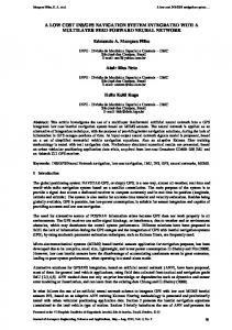
From this data, we can integrate to find relative speed and heading. This is discussed in more detail in the chapter on system modeling. An example plot of the inertial sensor outputs for a 10-second time frame is shown in Figure 3.6.
9
Inertial Sensor Outputs vs Time
Sensor Output (millivolts)
3500 Fwd/Rev
3300
Gyroscope
3100
Steering Potentiometer
2900
Side Accelerometer
2700 Vehicle turning
Vehicle decelerating
2500 1
101
201
301
401
501
601
701
801
901
1001
Time (hundreths of seconds) Figure 3.6 – Example plot of inertial sensor outputs
3.4 Data Acquisition Board The data acquisition board we used on this project was a Iotech DaqBook 100. It is a small box that sits outside the PC, and attaches to the PC via a parallel cable. All of our sensor inputs are connected into the three connectors on the back of the DaqBook – one analog I/O, one digital I/O, and one pulse/frequency/high-speed digital input. Our two gyroscopes (even though one was not operational), two accelerometers Status indicator lights Parallel PC interface
and steering potentiometer all input to the analog I/O port. The single distance encoder output (we used either the odometer input or the ABS input at any one time) fed into the pulse digital
Figure 3.7 – Close-up picture of the DaqBook
input. The DaqBook analog inputs can
10
be set to operate in differential or single-ended mode. This means that analog signals can be measured based on the potential between the single pin’s input and the DaqBook’s ground (single-ended) or the signals can be measured based on the potential between adjacent pins (differential). In addition, the board can be set to measure analog inputs as unipolar or bipolar. In unipolar mode, input voltages from 0 to +10 volts can be applied, and in bipolar mode, input voltages of up to 5 volts in magnitude in either polarity can be applied. Each of the analog pins we set to operate in differential, unipolar mode. When the DaqBook is connected to a standard parallel port, it supports up to 170 Kbytes/sec of bi-directional communication. We are sampling data at 100 Hz in this project, and each sample is 14 bytes of data, resulting in 11.2 Kbytes/sec of data transferred. Any commands sent to the board must also be considered, but we can see that the board can easily handle the data rate we desire. More about the data samples will be presented in the software chapter of this thesis. (DaqBook, 1994) The data acquisition board can be used in several different modes, but we essentially used only two: polled output, and timed output. In DOS based programming, we are less encumbered by delays introduced by the operating system (OS) on I/O operations, such as parallel port reads and writes. For this reason, we are able to use polled output from the DaqBook, which is substantially easier to implement. A 100 Hz loop is implemented using interrupt based timing in the host computer, and in each loop we send a request and receive a response with negligible delay. When programming under Windows 95, which is not truly a real-time OS, we found that we could not use the simple polled-response method that worked with DOS. After a little work, we found that the DaqBook could be set to automatically sample data at a specified rate. This rate is maintained by internal timing circuitry, so our program did not need to initiate each sample. The program merely ‘grabbed’ the data sample from the parallel port at the appropriate time. More details about the implementation in the programs are presented in the chapter on software.
11
3.5 GPS Receiver Perhaps the single most important piece of hardware in this system is the GPS receiver. The output from the receiver is the only way we have any notion of our absolute position on the globe. For information regarding some basic GPS fundamentals, refer to Appendix C.
Figure 3.8 – Motorola VP Oncore GPS Receiver (from Motorola Oncore User’s Guide)
The GPS receiver used in this project was a Motorola VP Oncore 6-channel receiver. This version of the Oncore receiver communicates serially via a transistortransistor logic (TTL) interface with the host computer at 9600 baud. The receiver has the capability to perform differential GPS (DGPS) given the appropriate input from a source such as a Coast Guard DGPS station. We did not use this feature since it required additional hardware, a Coast Guard beacon receiver, and because differential correction signals are not available everywhere. We used the GPS receiver in a very simple manner. The receiver can be set such that it automatically sends its complete message once every second. It is then the job of the host computer to detect the message and interpret it correctly. From this data, we know our current position, time, and status information for the receiver. The receiver is capable of receiving and processing dozens of user commands, but for our purposes, the automatic once-per-second output is adequate. For more information about the Motorola Binary Format messages, refer to Appendix C. When processing the sensor data, we would like to know whether the GPS data being returned is likely to be ‘good’ or not. A simply method of determining this is based on the status information returned from the
12
receiver with each data message. The GPS receiver returns a status byte with the following information: Bit Bit Bit Bit Bit Bit Bit Bit
7: 6: 5: 4: 3: 2: 1: 0:
Position propagate mode Poor geometry (DOP > 20) 3D fix Altitude hold (2D fix) Acquiring satellites/position hold Differential Insufficient visible satellites (=0x10000L){ /* roughly 1/18.2 sec has elapsed */ clock_ticks-=0x10000L; (*BIOSTimerHandler)(); /* call the system timer handler */ } else outp(0x20,0x20); /* clear interrupt and continue */ }
The keywords __interrupt and __far tell the compiler explicitly how to handle the function. The keyword __interrupt tells the compiler that this function is meant to be called as an ISR, because the compiler must add special assembly calls to properly
54
return from an ISR. The keyword __far tells the compiler that this function may be called from outside of the current code segment. These keywords are specific to Borland C++ version 4.5, and may need to be changed for other compilers. Following are the code segments that initialize and clean up the system timer ISR, along with the global declaration for the variable BIOSTimerHandler, which is a pointer to hold the address of the system timer ISR. SetTimer is called at the beginning of the program to setup the PIT chip and new timer ISR jump vector, and CleanUpTimer is called to reset the PIT chip and old timer ISR jump vector. A jump vector refers to a place in memory that holds the address of an ISR. Every time any interrupt is generated, the system looks at a predefined place in memory to find the address of the ISR, or jump vector. #define TIMERINTR #define PIT_FREQ
0x08 0x1234DDL
/* timer interrupt jump vector location */ /* frequency of PIT chip */
void __interrupt(__far *BIOSTimerHandler)(void);
/* old timer ISR pointer */
void SetTimer(void interrupt(__far *TimerHandler)(void), int frequency){ clock_ticks=0; /* initialize clock counter */ counter=(long)PIT_FREQ/frequency; /* determine PIT divisor */ BIOSTimerHandler=getvect(TIMERINTR); /* get address of old timer handler */ setvect(TIMERINTR,TimerHandler); /* set 100 Hz timer handler jump vector */ outp(0x43,0x34); /* set PIT chip frequency */ outp(0x40,counter%256); /* output low byte of counter value */ outp(0x40,counter/256); /* output high byte of counter value */ } void CleanUpTimer(void){ outp(0x43,0x34); /* outputting 0x0000 to the PIT chip outp(0x40,0x00); outp(0x40,0x00); setvect(TIMERINTR,BIOSTimerHandler); }
/* reset PIT chip frequency */ sets the maximum counter value of 0x10000 */ /* send low byte of counter value */ /* send high byte of counter value */ /* set old timer handler jump vector */
The following table contains a list of many of the important system interrupts that can be called, as listed in Programmer’s Problem Solver (Jourdain, 1992).
55
Vector 00h 01h 02h 03h 04h 05h 06h 07h 08h 09h 0Ah 0Bh 0Ch 0Dh 0Eh 0Fh 10h 11h 12h 13h
Function Divide by zero error Processor single step Nonmaskable interrupt Processor break point Processor overflow Print screen Unused Unused Timer (time-of-day count) Keyboard Reserved COM2 COM1 Hard disk drive controller Diskette drive controller Printer controller Video driver Equipment configuration check Memory size check Disk I/O (PC/XT)
Vector 14h 15h 16h 17h 18h 19h 1Ah 1Bh 1Ch 1Dh 1Eh 1Fh 20h 21h 22h 23h 24h 25h 26h 27h
Function Com port driver Network & miscellaneous services Keyboard buffer access Printer access ROM BASIC System restart Timer & real-time clock access Ctrl-Break handler User defined timer tick routine Video parameter table Disk parameter table Graphics character table Program terminate DOS functions Terminate vector Ctrl-C vector Critical-error vector Absolute disk sector read Absolute disk sector write Terminate and stay resident
6.2.2 Com Port Interrupt Programming Activating the ISR for com port programming is quite similar to activating the ISR for the system timer. The functions SetCom1 and CleanUpCom1 are analogous to SetTimer and CleanUpTimer, described in the section above. These functions are shown here: #define #define #define #define #define
COM1INTR GPS_PORT_DATA GPS_PORT_STATUS GPS_PORT_INTR GPS_PORT_CONT
0x0C 0x3F8 0x3FD 0x3F9 0x3FC
/* /* /* /* /*
com port ISR jump vector number */ port where data arrives */ line status register */ interrupt enable register */ modem control register */
void SetCom1(void interrupt(__far *ComHandler)(void)){ BIOSCom1Handler=getvect(COM1INTR); /* get old com ISR handler */ setvect(COM1INTR,ComHandler); /* set new com ISR handler */ gps_port_intr_set=inportb(GPS_PORT_INTR); /* get initial port settings */ outportb(GPS_PORT_CONT,11); /* assert DTR and RTS signals */ outportb(GPS_PORT_INTR,1); /* set to interrupt on data received */ inportb(GPS_PORT_DATA); /* clear any pending data on com port */ outp(0x21,inportb(0x21)&0xEF); } void CleanUpCom1(void){ outportb(GPS_PORT_INTR,gps_port_intr_set); /* return initial port settings */ setvect(COM1INTR,BIOSCom1Handler); /* set old com ISR handler */ }
56
Note that SetCom1 does more than just set the jump vector for the ISR. It also must do some setup specifically for the com port. Most importantly, it sets the com port to generate an interrupt (which is then handled by our ISR) whenever a data byte has arrived on the port. Likewise, the ISR for the com port must do more than set a flag. At any given time, our program is unaware of where we are in the message from the GPS receiver. For this reason, the interrupt handler must be able to synchronize itself with the GPS message. Synchronization is accomplished by finding a known sequence of characters in the message, then orienting the rest of the message by this sequence. We implement this by means of input states. Initially, we are in state 0 waiting for the first character in the sequence, which is a @ character. Once we get the character, we advance to state 1, where we again wait for a @ character. Then we wait for a B in the same way. If the sequence fails to match the expected @@B at any point, we return to state 0. After the start sequence has been detected, we assume that we are synchronized with the GPS receiver and collect the remainder of the fixed-length message. Once the entire message has been collected, we set a flag indicating that the main program should interpret the message. The state diagram for the com input is shown in Figure 6.3. (c!=’@’) i=0
(c==’@’) i=1
1
(c==’@’) i=2
2
(c==’B’) i=3
3
(i < 68) i++
4
(c!=’@’) i=0 (c!=’B’) i=0 (i == 68) set ‘done’ flag i=0 Figure 6.3 – Serial com state diagram for GPS data input
Note that the sequence detection and message gathering must be done in the com port ISR, instead of simply setting a flag each time a character is received and having the main program handle it. This is because our main program is running at 100 Hz due to the timer interrupt, while we receive data bytes at nearly 10 times that rate. However, the com port input is in bursts of 68 characters at 1 Hz. This means that our program has time
57
to run at least one 100 Hz loop and interpret the received message before the next message is begun. Despite this long discussion of the ISR, the actual implementation is quite simple. The com port ISR code is shown here: void __interrupt __far Com1Handler(void){ gps_char=inportb(GPS_PORT_DATA); /* retrieve data from com port */ if(!new_gps){ switch(gps_report_idx){ /* depending on what state we’re in... */ case 0: case 1: /* waiting for message beginning (@@) */ if(gps_char=='@'){ gps_report[gps_report_idx]='@'; gps_report_idx++; } break; case 2: /* waiting for ‘B’ character */ if(gps_char!='B') gps_report_idx=0; else{ gps_report[gps_report_idx]='B'; gps_report_idx++; } break; default: /* waiting for remainder of message */ gps_report[gps_report_idx]=gps_char; gps_report_idx++; break; } if(gps_report_idx==68){ /* if message complete... */ gps_report_idx=0; /* reset message index for next message */ new_gps=1; /* set flag to indicate complete message */ } } outp(0x20,0x20); /* clear interrupt */ }
6.2.3 VGA Output In the interest of keeping the software as simple and fast as possible, while still providing some graphical feedback, we used the video mode known as Mode 13. Many older DOS based video games use Mode 13 because it is very simple and easy to implement on any PC. We implemented a very low-level pixel plot routine, and from it built routines to plot lines, boxes, and text. This section will cover only the basics of Mode 13 operation. Mode 13 is a 320x200 resolution graphics video mode which every graphics card supports. Video memory for this mode is represented as a single contiguous segment of memory starting at location A0000 hex. Each pixel is a single byte in the array, so the entire screen is 64000 (320x200) bytes in size. Colors are produced by maintaining a palette of 256 color values. The palette is a series of 256 three-byte triplets defining the
58
red, green, and blue components for each entry. Thus, the mode is capable of representing 16.8 million (2563) different colors, but only 256 at a time. (Mazidi and Mazidi, 1995) Initializing the video mode to Mode 13 is very simple. We need only to put the value 13 hex into the ax CPU register and generate the BIOS interrupt 10 hex. This is shown in the function set_vga: void set_vga(void){ asm{ pusha mov ax,0x0013 int 0x10 popa } }
// // // //
store the A register so we don’t mess it up load 0x13 into the A register (VGA mode) call the BIOS interrupt to set mode 0x13 restore the A register
Resetting the mode to the text mode, which we are used to, is just as simple. We just put 03 hex into the ax register and generate the same interrupt. This is shown in the function set_text: void set_text(void){ asm{ pusha mov ax,0x0003 int 0x10 popa } }
// // // //
store the A register so we don’t mess it up load 0x03 into the A register (text mode) call the BIOS interrupt to set mode 0x03 restore the A register
After the mode has been initialized, plotting a pixel is as simple as writing the color byte to the appropriate position in memory. The video memory array starts at the upper-left corner of the screen, runs across the screen line-by-line, and ends at the lowerright corner of the screen. (LaMothe et al., 1994) …… Increasing X index Increasing Y index
Figure 6.4 – VGA screen memory orientation
So we orient our coordinate system such that the x-axis starts on the left and points right, while our y-axis starts at the top and points down. Thus, if we want to plot a point at the position (x,y), we simply write to the array at offset [y*320 + x]. The 59
routine blit_bit plots a pixel of value color to the screen at position (x,y). A pointer to the screen memory is passed in vscreen, which is always A0000 hex. A common way to calculate the offset into the array is to use bit-shifts, rather than a multiplication. Note that y*320 is equal to y*256+y*64, which may also be written as yRead(&m_NextGPSTime,sizeof(unsigned int))!= sizeof(unsigned int)) { m_pMainPage->SetRunState(FALSE); return TRUE; } m_pGPSFile->Read(&m_NextGPSData,sizeof(T_POS_CHAN_STATUS)); memcpy(&m_CurrGPSData,&m_NextGPSData,sizeof(T_POS_CHAN_STATUS)); m_CurrGPSTime = m_NextGPSTime; m_GPSLatitude=(int)((m_CurrGPSData.latitude.seconds+ m_CurrGPSData.latitude.minutes*60.0+ abs(m_CurrGPSData.latitude.degrees)*3600.0)*1000.0)* SGN((m_CurrGPSData.latitude.degrees)); m_GPSLongitude=(int)((m_CurrGPSData.longitude.seconds+ m_CurrGPSData.longitude.minutes*60.0+ abs(m_CurrGPSData.longitude.degrees)*3600.0)*1000.0)* SGN((m_CurrGPSData.longitude.degrees)); if((m_CurrGPSData.rcvr_status & 0x43) ||
110
!(m_CurrGPSData.rcvr_status & 0x30)) m_GPSGood = FALSE; else m_GPSGood = TRUE; m_pGPSPage->m_GoodGPSCheckVar = m_GPSGood; m_pGPSPage->UpdateContents(); } // run Filter100Hz (for sensor data) -> update sensor page if(m_pMainPage->m_HertzEditVar && !(m_RunCount%(m_pMainPage->m_HertzEditVar/10))) m_pSensorPage->UpdateContents(); else if(!(m_RunCount%50)) m_pSensorPage->UpdateContents(); Filter100Hz();
// execute the inertial sensor filter
// if time on sensor>=next GPS time (synchronize GPS and inertial data) if(m_CurrSensorData.ticks>=m_NextGPSTime) { // copy m_NextGPSData to m_CurrGPSData memcpy(&m_CurrGPSData,&m_NextGPSData,sizeof(T_POS_CHAN_STATUS)); m_CurrGPSTime = m_NextGPSTime; // update m_GPSLatitude, m_GPSLongitude, and m_GPSGood m_GPSLatitude=(int)((m_CurrGPSData.latitude.seconds+ m_CurrGPSData.latitude.minutes*60.0+ abs(m_CurrGPSData.latitude.degrees)*3600.0)*1000.0)* SGN((m_CurrGPSData.latitude.degrees)); m_GPSLongitude=(int)((m_CurrGPSData.longitude.seconds+ m_CurrGPSData.longitude.minutes*60.0+ abs(m_CurrGPSData.longitude.degrees)*3600.0)*1000.0)* SGN((m_CurrGPSData.longitude.degrees)); if((m_CurrGPSData.rcvr_status & 0x43) || !(m_CurrGPSData.rcvr_status & 0x30)) m_GPSGood = FALSE; else m_GPSGood = TRUE; // update GPS page (w/ new current GPS data) m_pGPSPage->m_GoodGPSCheckVar = m_GPSGood; m_pMapDlg-> PlotRawGPS(CPoint(m_GPSLongitude,m_GPSLatitude),m_GPSGood); // -> update output window m_pGPSPage->UpdateContents(); // Filter1Hz (for GPS data) if(!m_Fuzzy) Filter1Hz(); // use rule-based fusion else Fuzzy1Hz(); // use fuzzy fusion // read next GPS data into m_NextGPSData if(m_pGPSFile->Read(&m_NextGPSTime,sizeof(unsigned int)) !=sizeof(unsigned int)) { m_pMainPage->SetRunState(FALSE); return TRUE; } m_pGPSFile->Read(&m_NextGPSData,sizeof(T_POS_CHAN_STATUS)); } // sleep to effect a pseudo-accurate timing if(m_pMainPage->m_HertzEditVar) Sleep(1000/(m_pMainPage->m_HertzEditVar)); } else Sleep(100); // keep from bogging down system in tight loop return TRUE;
// return TRUE so that OnIdle is called again
}
111
void CPostViewApp::InitFilter(void) { int i,j; // do anything related to initializing the filter here // (just to distinguish filter related initialization) // allocate vectors and matrices xk = vector(1,8); xkm1 = vector(1,8); yk = vector(1,2); Ak = matrix(1,8,1,8); Kk = matrix(1,8,1,2); C = matrix(1,2,1,8); Pk = matrix(1,8,1,8); Pk1 = matrix(1,8,1,8); Pkm1 = matrix(1,8,1,8); R = matrix(1,2,1,2); Q = matrix(1,8,1,8); mtemp1=matrix(1,8,1,8); mtemp2=matrix(1,8,1,8); mtemp3=matrix(1,2,1,8); mtemp4=matrix(1,2,1,2); mtemp5=matrix(1,2,1,2); mtemp6=matrix(1,2,1,2); mtemp7=matrix(1,8,1,2); mtemp8=matrix(1,2,1,8); mtemp9=vector(1,2); mtemp10=vector(1,2); mtemp11=vector(1,8); mtemp12=vector(1,8); mtemp13=matrix(1,8,1,8); mtemp14=matrix(1,8,1,8); // fill in intial values for Ak,C,Pkm1,Q,R // leave xkm1 all 0's until good GPS // initialize state transition matrix for(i=1;i put measurement variables into yk // (yk[1] = dtheta and yk[2] = odo_measure) double dtheta1 = ((m_GyroCenter-m_CurrSensorData.gyro1)/m_MvoltPerDegree); double odo_measure = (m_CurrSensorData.odometer_totalold_odo_total)/m_TicksPerMeter; if(odo_measurem_MaxDistPer100) odo_measure=0; old_odo_total=m_CurrSensorData.odometer_total; if(odo_measure==0) odo_zero_count++; else odo_zero_count=0; if(odo_zero_count>20) m_GyroCenter= m_GyroCenter*0.98+m_CurrSensorData.gyro1*0.02; if(ABS(m_CurrSensorData.steer-m_SteerCenter) generate system transfer by linearizing non-linear functions (Ak) Ak[1][6]=cos(DEG_TO_RAD(xkm1[3]))*meters_to_msec_long; Ak[2][6]=sin(DEG_TO_RAD(xkm1[3]))*meters_to_msec_lat;
//
m_LastGoodGPSDLat += Ak[2][6]*odo_measure; m_LastGoodGPSDLong += Ak[1][6]*odo_measure; // -> generate measurement transfer by linearizing non-linear functions (Ck) // -> predict error covariance // (Pk1 = Ak * Pkm1 * AkT + Q) mat_mult(Ak,Pkm1,mtemp1,8,8,8); mat_mult_transpose(mtemp1,Ak,mtemp2,8,8,8); mat_add(mtemp2,Q,Pk1,8,8); // -> find Kalman gain based on predicted error covariance // (Kk = Pk1 * CT * [C * Pk1 * CT + R]^-1) mat_mult(C,Pk1,mtemp3,2,8,8); mat_mult_transpose(mtemp3,C,mtemp4,2,8,2); mat_add(mtemp4,R,mtemp5,2,2); mat_inverse(mtemp5,mtemp6,2); mat_mult_transpose(Pk1,C,mtemp7,8,8,2); mat_mult(mtemp7,mtemp6,Kk,8,2,2); // -> estimate state based on old state, and difference // between predicted observations and actual observations // (xk = Ak * xkm1 + Kk * (yk - C * Ak * xkm1) mat_mult(C,Ak,mtemp8,2,8,8); mat_mult_vector(mtemp8,xkm1,mtemp9,2,8); vec_sub(yk,mtemp9,mtemp10,2); mat_mult_vector(Kk,mtemp10,mtemp11,8,2); mat_mult_vector(Ak,xkm1,mtemp12,8,8); vec_add(mtemp12,mtemp11,xk,8); // -> get error covariance // (Pk = Pk1 - Kk * C * Pk1)
118
mat_mult(Kk,C,mtemp13,8,2,8); mat_mult(mtemp13,Pk1,mtemp14,8,8,8); mat_sub(Pk1,mtemp14,Pk,8,8); // -> current state values are in xk // (longitude = xk[1] and latitude = xk[2]) if(m_DebugOut) { // print a bunch of stuff to a file for debug puposes char str[150]; int i; for(i=0;iWrite(str,strlen(str)); } sprintf(str,"\n"); if(m_DebugFile!=NULL) m_DebugFile->Write(str,strlen(str)); } // -> update for next time // (xkm1 = xk) // (Pkm1 = Pk) mat_copy(Pk,Pkm1,8,8); vec_copy(xk,xkm1,8); filter_count++; m_fxkValid = TRUE; } }
119
Vita David McNeil Mayhew was born on September 15, 1976 in Dale City, Virginia. He attended North Stafford High School and graduated in 1994. David entered Virginia Polytechnic Institute and State University as an undergraduate in the Engineering program in fall of 1994. David graduated with his Bachelor of Science in Computer Engineering in December of 1997. David then remained at Virginia Tech and completed his Masters of Science Degree in Electrical Engineering in the summer of 1999. David has taken an engineering position with Intelligent Automation Inc., a robotics and artificial intelligence research and development company located in Rockville, Maryland.
120