Multi-Robot Formations for Area Coverage in Space Applications

AB

TEKNILLINEN KORKEAKOULU Faculty of Electronics, Communications and Automation Department of Automation and Systems Technology

Jürgen Leitner

Multi-Robot Formations for Area Coverage in Space Applications Thesis submitted in partial fulfilment of the requirements for the degree of Master of Science in Technology Espoo, August 17, 2009

Supervisors: Professor Aarne Halme

Professor Kalevi Hyyppä

Helsinki University of Technology

Luleå University of Technology

Instructor: Tapio Taipalus

Professor Shinichi Nakasuka


The University of Tokyo

Parts of this thesis were done at the University of Tokyo’s Intelligent Space Systems Laboratory supported by the SpaceMaster Global Partnership Programme.

Acknowledgements Firstly I want to thank everybody involved in the SpaceMaster programme and everybody I met during these unforgettable last two years. Especially I want to thank my supervisor, Professor Aarne Halme, who allowed me to pursue a research in cooperation with the Intelligent Space Systems Laboratory, at the University of Tokyo. I want to thank Professor Shinichi Nakasuka for providing me with the possibility to work and do research at his lab in Tokyo for 3 months, as well as helping me with the various problems arising during my thesis. It was an amazing experience and I will never forget it! I also want to thank Professor Keiki Takadama and his students for surviving a very long presentation about me and my thesis at the University of Electro-Communications in Chofu and for helping me, especially with the machine learning part of the thesis. I would also like to thank my instructor Tapio Taipalus and Marek Matusiak for their guidance in selecting, researching, and implementing this thesis. Also thanks to Professor Kalevi Hyyppä for feedback on early thesis drafts. I am especially grateful for the SpaceMaster consortium, to chose me to become part of Round 3, and the European Union, for creating the Erasmus Mundus programmes. Apart from doing a great job to organize multiple universities and create a unique educational experience, it is also an amazing personal experience. I found some really good friends during the time of the course. The financial support received by foremost my parents, but also the European Space Agency, with a scholarship during the first year, and the European Union, with an ERASMUS scholarship via the Julius-Maximilians Universität ii

Würzburg throughout the second year and a special ‘SpaceMaster Global Partnership’ scholarship for my stay in Japan, is greatly appreciated. I also want to thank the reviewers and organizers of the 2009 International Conference on Automation, Robotics and Control Systems (ARCS-09) and The 2009 ECSIS Symposium on Learning and Adaptive Behavior in Robotic Systems (LAB-RS 2009) for giving me lots of feedback and publishing my papers, based on seminar work and literature review. The registration for those events was generously sponsored by Prof. Nakasaka’s lab in Tokyo. Special thanks go to David Leal Martínez and Melak Mekonen Zebenay, for their discussions and coffee breaks, which yielded great input and good relaxation. David also deservers another huge Thank You for providing me with his robots to test my algorithm on, as well as arranging our participation at the 2009 International Joint Conference in Artificial Intelligence, Robotics Exhibition Workshop (IJCAI-09) in Pasadena. Also I want to thank William Martin, for proof-reading my seminar work and this thesis. He also gave additional feedback on style and formatting which were greatly appreciated. I also want to thank my family and girlfriend for proof-reading, trying to understand the idea behind this thesis and not fall asleep during presentation test runs :) I am very thankful for all the support from my parents, brother, relatives and friends along the way. I would not be where I am right now without all of them. Thank You!

Jürgen Leitner Espoo, July 31, 2009

iii


Abstract of the Master’s Thesis

Author:

Jürgen Leitner

Title of the thesis:

Multi-Robot Formations for Area Coverage in Space Applications

Date:

August 9, 2009

Number of pages: 99

Faculty:

Faculty of Electronics, Communications and Automation

Department:

Automation and System Technology

Programme:

Master’s Degree Programme in Space Science and Technology

Professorship:

Automation Technology (Aut-84)

Supervisors:

Professor Aarne Halme (TKK) Professor Kalevi Hyyppä (LTU)

Instructor:

Professor Shinichi Nakasuka (ISSL) Tapio Taipalus (TKK)

This thesis presents two algorithmic implementations of multi-robot formation control for the area coverage problem. It uses a space exploration scenario, with a marsupial robot society, for tasks like mapping, habitat construction, etc. The solutions are though applicable to a wider range of applications, since area coverage is seen as one of the canonical problems in multi-robot application. Starting with an overview of multi-robot systems in space applications, both currently in use and planned for the near future, it then presents the two algorithms and their implementation in C++: (i) a vector force based implementation and (ii) a machine learning approach. The second is based on an organizational-learning oriented classifier system (OCS) introduced by Takadama an evolution of Holland’s learning classifier system (LCS). To ease the development, testing and evaluation of the control algorithms a simulator, named SMRTCTRL, was implemented during a 3 months research stay at the University of Tokyo. The vector-based control approach was tested using a multi-robot society of LEGO Mindstorms Robots and a comparison of the two algorithm was done with the help of the simulator. Keywords:

space robotics, multi-robot cooperation, area coverage, machine learning, simulation, formation control, Learning Classifier Systems (LCS)

iv

Contents 1 Introduction

1

1.1 Multi-Robot Scenarios for Space Exploration . . . . . . . . . . .

2

1.2 What is Cooperation? . . . . . . . . . . . . . . . . . . . . . . .

4

1.3 Thesis Motivation, Approach and Goal . . . . . . . . . . . . . .

6

1.4 Thesis Outline . . . . . . . . . . . . . . . . . . . . . . . . . . . .

7

2 Related Work

8

2.1 Introduction . . . . . . . . . . . . . . . . . . . . . . . . . . . . .

8

2.2 Multi-Robot Cooperation . . . . . . . . . . . . . . . . . . . . . .

9

2.2.1

Introduction . . . . . . . . . . . . . . . . . . . . . . . . .

9

2.2.2

Taxonomy . . . . . . . . . . . . . . . . . . . . . . . . . .

10

2.2.3

Applications in Space . . . . . . . . . . . . . . . . . . . .

15

2.3 Coverage . . . . . . . . . . . . . . . . . . . . . . . . . . . . . . .

28

2.3.1

Art Gallery Problem . . . . . . . . . . . . . . . . . . . .

30

2.3.2

Boustrophedon Cellular Decomposition . . . . . . . . . .

30

2.3.3

Distributed Coverage Experiments . . . . . . . . . . . .

31

3 Problem Formulation

33

3.1 Overview . . . . . . . . . . . . . . . . . . . . . . . . . . . . . . .

33

3.2 Boundary Conditions . . . . . . . . . . . . . . . . . . . . . . . .

35

3.2.1

Marsupial Robot Society . . . . . . . . . . . . . . . . . .

35

3.2.2

Robot Localization and Global Map . . . . . . . . . . . .

37

3.2.3

Terrain and Robot Motion . . . . . . . . . . . . . . . . .

38

3.2.4

Sensor Model . . . . . . . . . . . . . . . . . . . . . . . .

39

3.3 Multi-Robot Architecture . . . . . . . . . . . . . . . . . . . . .

40

3.4 Optimization Conditions . . . . . . . . . . . . . . . . . . . . . .

40

3.5 Mathematical Formulation of the Coverage Problem . . . . . . .

41

v

4 Algorithm

43

4.1 Overview . . . . . . . . . . . . . . . . . . . . . . . . . . . . . . .

43

4.2 Theoretical Background . . . . . . . . . . . . . . . . . . . . . .

44

4.2.1

Machine Learning . . . . . . . . . . . . . . . . . . . . . .

44

4.2.2

Vector-Based Formations . . . . . . . . . . . . . . . . . .

51

4.2.3

Multi-Agent-Systems Architectures . . . . . . . . . . . .

53

4.3 Placement Using Force Vectors . . . . . . . . . . . . . . . . . .

56

4.4 Placement Using Machine Learning . . . . . . . . . . . . . . . .

57

4.4.1

Pseudo-Code . . . . . . . . . . . . . . . . . . . . . . . .

58

4.4.2

Classifier Design

. . . . . . . . . . . . . . . . . . . . . .

61

4.4.3

Memories, Mechanisms and the Environment Model . . .

62

4.4.4

The COCSMover Class . . . . . . . . . . . . . . . . . . .

66

4.5 Optimization . . . . . . . . . . . . . . . . . . . . . . . . . . . .

67

4.6 Changes in Formation . . . . . . . . . . . . . . . . . . . . . . .

68

4.7 Coverage Calculation Math . . . . . . . . . . . . . . . . . . . .

69

5 Simulator

70

5.1 Overview . . . . . . . . . . . . . . . . . . . . . . . . . . . . . . .

70

5.2 Internal Design . . . . . . . . . . . . . . . . . . . . . . . . . . .

73

5.3 Discrete vs. Continuous Simulation . . . . . . . . . . . . . . . .

73

5.4 Visualization . . . . . . . . . . . . . . . . . . . . . . . . . . . .

74

6 Results

78

6.1 Standard Initial Configuration . . . . . . . . . . . . . . . . . . .

78

6.2 Robot Placement . . . . . . . . . . . . . . . . . . . . . . . . . .

79

6.2.1

Vector-Based Simulation Results . . . . . . . . . . . . .

79

6.2.2

Machine Learning Simulation Results . . . . . . . . . . .

81

6.2.3

Comparison . . . . . . . . . . . . . . . . . . . . . . . . .

83

6.3 Project SMURFS at IJCAI . . . . . . . . . . . . . . . . . . . .

84

6.3.1

Experimental Findings . . . . . . . . . . . . . . . . . . .

85

6.4 Adaption . . . . . . . . . . . . . . . . . . . . . . . . . . . . . . .

87

7 Summary and Conclusions

88

7.1 Future Work . . . . . . . . . . . . . . . . . . . . . . . . . . . . .

vi

90

References

91

A Mathematical Representations A.1 Ellipses

I

. . . . . . . . . . . . . . . . . . . . . . . . . . . . . . .

A.2 Vectors and Force Representations

I

. . . . . . . . . . . . . . . . III

B liglui - An SDL GUI Library

IV

C UML Diagrams

V

C.1 The Simulator Class Diagram . . . . . . . . . . . . . . . . . . .

V

C.2 The Simulator Sequence Diagram . . . . . . . . . . . . . . . . .

V

C.3 The Robot Control Class Diagram . . . . . . . . . . . . . . . . .

V

D Simulator

IX

D.1 Internal Design . . . . . . . . . . . . . . . . . . . . . . . . . . . IX D.2 Visualization . . . . . . . . . . . . . . . . . . . . . . . . . . . . XV E Source Code Listings

XX

vii

List of Tables 2.1 Multi-Robot Taxonomy Axes . . . . . . . . . . . . . . . . . . .

12

3.1 Marsupial (Marsubot) Specifications . . . . . . . . . . . . . . . .

36

3.2 The Robots’ Simplified Motion . . . . . . . . . . . . . . . . . .

39

6.1 Vector-Based Simulation Results . . . . . . . . . . . . . . . . . .

80

6.2 Algorithm Comparison . . . . . . . . . . . . . . . . . . . . . . .

83

List of Figures 1.1 Illustration of Lunar and Martian Outposts . . . . . . . . . . .

3

2.1 ATV Docking . . . . . . . . . . . . . . . . . . . . . . . . . . . .

16

2.2 Satellite Formation Flying Types . . . . . . . . . . . . . . . . .

17

2.3 Trailing Formation, LANDSAT-7 and EO-1 . . . . . . . . . . .

18

2.4 A-train Formation

. . . . . . . . . . . . . . . . . . . . . . . . .

19

2.5 LISA Satellite Formation . . . . . . . . . . . . . . . . . . . . . .

22

2.6 MetNet Lander Concept . . . . . . . . . . . . . . . . . . . . . .

23

2.7 LEMUR Marsupial Robot Concept . . . . . . . . . . . . . . . .

26

2.8 Art Gallery Problem . . . . . . . . . . . . . . . . . . . . . . . .

30

2.9 Boustrophedon Decomposition . . . . . . . . . . . . . . . . . . .

31

2.10 UAV Coverage Simulation . . . . . . . . . . . . . . . . . . . . .

32

3.1 Marsupial Robots at TKK . . . . . . . . . . . . . . . . . . . . .

34

viii

3.2 Marsubots Entering & Energy Docking . . . . . . . . . . . . . .

37

4.1 Reinforcement Learning Interactions . . . . . . . . . . . . . . .

46

4.2 Holland’s LCS . . . . . . . . . . . . . . . . . . . . . . . . . . . .

49

4.3 Takadama’s OCS . . . . . . . . . . . . . . . . . . . . . . . . . .

50

4.4 Vector Forces in a Robot Formation . . . . . . . . . . . . . . . .

52

4.5 TraderBots Architecture . . . . . . . . . . . . . . . . . . . . . .

55

4.6 Classifier Structure . . . . . . . . . . . . . . . . . . . . . . . . .

61

4.7 Illustration of the Learning Mechanisms in OCS . . . . . . . . .

65

5.1 Screenshot of the Simulator . . . . . . . . . . . . . . . . . . . .

72

5.2 Discrete vs. Continuous Visualization . . . . . . . . . . . . . . .

74

5.3 Terrain Representation . . . . . . . . . . . . . . . . . . . . . . .

76

6.1 Evolution of the ML Results . . . . . . . . . . . . . . . . . . . .

82

6.2 Simulation Result Comparison . . . . . . . . . . . . . . . . . . .

83

6.3 The Gargamel Tracking System . . . . . . . . . . . . . . . . . .

84

6.4 The reacTIvision server and the SMRTCTRL Simulator . . . .

85

6.5 Robot Movements: Real-World vs. Simulator . . . . . . . . . . .

86

A.1 Ellipse Representation Used . . . . . . . . . . . . . . . . . . . .

II

A.2 Vector Representation Used . . . . . . . . . . . . . . . . . . . . III B.1 GUI Components Classes . . . . . . . . . . . . . . . . . . . . . . IV C.1 Simulator Class Diagram . . . . . . . . . . . . . . . . . . . . . . VI C.2 Simulator Sequence Diagram . . . . . . . . . . . . . . . . . . . . VII C.3 Robot Control Class Diagram . . . . . . . . . . . . . . . . . . . VIII D.1 MVC Standard and Simulator Architecture Comparison . . . . .

X

D.2 Thread Start Sequence . . . . . . . . . . . . . . . . . . . . . . . XIV D.3 Target Area Definition Classes . . . . . . . . . . . . . . . . . . . XVII D.4 Terrain Interaction Effects . . . . . . . . . . . . . . . . . . . . . XVIII

ix

Symbols and Abbreviations A(pi )

Area Defined by the Polygon pi

ci

Cell i of the (Discrete) Target Area

Cov

Coverage Percentage

L, W

Length and Width of the Target Area

N

Natural Numbers

pi

Polygon (Coverage Area of Robot i)

R

Rational Numbers

Ψ

Covered (Target) Area

Ω

Target Area

ACT

Advanced Concepts Team, ESA

AI

Artificial Intelligence

ANN

Artificial Neural Network

ATV

Automatic Transfer Vehicle

CF

Classifier in an OCS

CMU

Carnegie Mellon University, Pittsburgh, USA

DAI

Distributed Artificial Intelligence

DEM

Digital Elevation Map

ESA

European Space Agency

FIRA

Federation of International Robot-soccer Association x

GA

Genetic Algorithm

GUI

Graphical User Interface

HST

Hubble Space Telescope

IJCAI

International Joint Conference on Artificial Intelligence

ISS

International Space Station

ISSL

Intelligent Space Systems Laboratory, The University of Tokyo

JAXA

Japan Aerospace Exploration Agency

JPL

NASA’s Jet Propulsion Laboratory

LASER

Light Amplification by Stimulated Emission of Radiation

LCS

Learning Classifier Systems

LTU

Luleå University of Technology, Sweden

ML

Machine Learning

MVC

Model-View-Controller

NASA

National Aeronautics and Space Administration, USA

OCS

Organizational-learning oriented Classifier System

RL

Reinforcement Learning

SDL

Simple DirectMedia Layer

SMRT

SpaceMaster Robotics Team

SMRTCTRL Simulator for Multi-RoboT ConTRoL SMURFS

Society of Multiple Robots

TKK

Helsinki University of Technology, Finland

UAV

Unmanned Aerial Vehicle

UML

Unified Modeling Language xi

Chapter 1 Introduction “We need dreamers ’cuz in our dreams we see not what is but what can be!.” - Juxi Leitner

The increasing pace of new developments in the field of robotics has led to quite stunning robots in the last decade. The evolution from quite limited industryrobots for construction and conveyor-belt work to the humanoid walking and learning robots, for example, Honda’s ASIMO in Japan, has not taken much more than 25 years. Robots are increasingly used in areas outside of designed and ‘easy’ environments, in areas where they need to interact with humans in some way. The need to be able to work in quite dynamic environments is frequently in the focus of robotics research. Another area, where robots are used nowadays and improve the return of scientific data, is space exploration with currently two active rovers deployed by NASA to scout the surface of Mars. The future is always hard to predict, but the current trend points towards more autonomous, more intelligent and more flexible robot systems working with, and supporting, humans in their daily life. One approach to reach this is the use of multiple, small robots working together towards a common goal. To ease the operation of those systems for human operators, autonomy is an important factor.

1.1 Multi-Robot Scenarios for Space Exploration

2

The use of cooperative robotics reaches technological constraints, even more than regular robotics, because of the need to cope with multiple, autonomous entities. At the same time it is highly inter-disciplinary and draws influences from many other fields of research, such as control theory, computer science, electronics, electro-communications, and artificial intelligence, as well as biology and social sciences. The use of robots in space, a generally very harsh environment, adds a new set of problems and constraints. Though this thesis focuses on the application in space exploration, it should be mentioned that these algorithms are useful in a wide variety of problems, ranging from multiple autonomous lawn-mowers, urban search and rescue (USAR), surveillance and scouting to (wireless) sensor deployment and cell-phone network coverage. Distributed coverage can hence be seen as one of the canonical problems in multi-robot applications.

1.1

Multi-Robot Scenarios for Space Exploration

An interesting scenario for multi-robot cooperation in space is the exploration of the Moon and Mars, where rovers are currently on the forefront of space exploration. Apart from a handful of people on the International Space Station just 300 km from Earth, these robots are the only way for humans to explore and experience space, especially at greater distances from Earth. The plans, presented by various space agencies, to create Lunar and Martian outposts for permanent human settlement will depend heavily on robotic reconnaissance, construction and operational support. Tasks for the robots will include mapping landing sites, constructing habitats and power plants, communicating with and acting as a communication relay to Earth, and so forth. Scenarios such as the ones depicted in Figure 1.1 show many different robots, with different, but overlapping, capabilities working together. One scenario for the use of multiple robots teaming up and working together can be taken from the recent (NASA, 2004) plans for building human outposts

1.1 Multi-Robot Scenarios for Space Exploration

3

on the Moon and Mars. These plans outline also a need for robotic support for the astronauts and explorers. In this scenario robots will, for example, search cooperatively for a location suitable in size and other properties to harbor a permanent human settlement. Several teams are formed once such a location is found, with each having a different task in the construction of the station. These tasks will include soil preparation and movement as well as, for example, carrying solar panels in tight-cooperation between two robots. The heterogeneity of the rovers is exploited throughout the whole mission to allow for better performance. Meanwhile, other rovers will begin with the exploration and surveying of the region around the construction site. Mission Control from Earth, together with the robots, then decides which areas are the most interesting for scientific research. Rovers with specialized sensing instruments are sent to investigate and cover as much of the area as possible, possibly transported in a larger mother-ship type robot at first. Formations of rovers will generate a wireless communication and emergency network for the robots as well as future human explorers. Robot failures are to be investigated by special diagnostic robots, which might even have possibilities to replace broken parts. In the meantime, robots with the same (or similar) capabilities are dispatched to minimize the interruptions.

Figure 1.1: Proposed Lunar and Martian outposts, showing multi-robot systems Courtesy: Astrobotic, NASA/JPL

1.2 What is Cooperation?

4

These autonomous systems can be used in various ways, forming groups dynamically, together with an autonomous task distribution system, to optimize the performance. The robots themselves will optimize their travel-time, waittime and the overall time-to-finish for a given task. Other ideas are: the establishing of long-life robotic science stations for continuous measurement and communications; construction of beaconed roadways and site preparation for human exploration as well as the deployment of human habitat modules. A self-sustaining outpost is favorable due the high cost of resupplying one such station from Earth. A scenario like this requires high performance from a heterogeneous multi-robot team in a very diverse and harsh environment. There are still many challenges to be tackled and obstacles to be overcome to be able to conduct such a mission by 2020 as planned by (NASA, 2004), but the recent developments of NASA systems, such as ATHLETE (and TriATHLETE), show gradual progress.

1.2

What is Cooperation?

The Oxford English Dictionary defines “to cooperate" as “to work together, act in conjunction (with another person or thing, to an end or purpose, or in a work)". In robotics, cooperation is not very often explicitly defined and the few definitions tend to be very broad, some including communication, and progressive results (e.g. increasing performance). The few exceptions are listed in (Cao et al., 1997) where also the following definition of a cooperative behavior in robotics is found: Given some task specified by a designer, a multiple-robot system displays cooperative behavior if, due to some underlying mechanism (i.e. the mechanism of cooperation), there is an increase in the total utility of the system. Cooperative and collaborative robotics started with the introduction of behavior based control into robotics. This paradigm is biologically inspired and

1.2 What is Cooperation?

5

encouraged researchers to find cooperating systems in nature, which then were used for multi-robot systems (Arai et al., 2002). Cooperation is also a very long and much discussed research topic in political science and other human sciences, see, for example, (Axelrod and Hamilton, 1981). Cooperating behaviors are a subset of collective behaviors, in which the cooperation can be manifold and usually is not clearly defined. Examples of cooperating in nature (e.g. bees and ants) show possibilities for simple robots to work together to solve a very complex task. The mechanism of cooperation may be incorporated into the system in various ways, by dynamics, by design or it may appear by accident. The first works on multi-robot cooperation appeared in the 1980s and the beginning of the 90s, see the CEBOT (Fukuda and Nakagawa, 1988) and SWARM (Beni, 1988) projects and (Von Martial, 1989; Fraichard and Demazeau, 1990). Recent advances in the field of cooperation come from robot soccer (Asada et al., 1999), where the limits of mechanical and electronic supremacy are reached, and games are more often won due to cooperation and teamwork1 . It contrast to the low level control of the robot (e.g. motion), cooperation can be seen as high level control, involving task and motion planning, task sharing, formations and the like. Cooperation does need the lower layers, such as obstacle avoidance, mapping, motion, and power management, since robots that cooperate still need local control, for example, local path planning and execution, collision avoidance, and obstacle detection. A formation can be seen as the simplest form of cooperation between autonomous robots.

1

see the results and papers published at the RoboCup and Federation of International

Robot-soccer Association (FIRA) conferences

1.3 Thesis Motivation, Approach and Goal

1.3

6

Thesis Motivation, Approach and Goal

As shown above, groups of robots offer the potential for increased performance and robustness for several applications. With an increasing amount of robots the control techniques used for these systems also increase in complexity. Therefore to make these multi-robot societies a useful addition to, for example, human space exploration, autonomous control needs to be added. The task of area coverage, is chosen as the representative case in multi-robot interaction throughout this thesis. The robots try to cover an area to provide, for example, a mobile communication infrastructure. The coverage problem is usually defined as to “cover a search space consistently and uniformly” (Menezes et al., 2007) and was first described for a team of robots by (Gage, 1992). For research done in multi-robot coverage, a problem area in the field of cooperative robotics, the problem can be interpreted as the ‘‘maneuvering of the robots into positions to keep the area constantly under good coverage with their sensors”, which can be seen as a high level formation control of robots. This thesis aims to compare a machine-learning (ML) based algorithm with a quite simple and lightweight vector-based algorithm for controlling the robots in an optimal way. The main questions are “Which of the two algorithms allows for better coverage?”, “Which one can optimize the solution, for example, to consume minimal fuel?” and “Which of the algorithms provides better solutions when reacting to changes in the environment?”. The latter question could not be answered, due to time constraints. The scenario would have been that one robot fails during operation and the systems’ response to it (i.e. the change in the coverage formation) would be evaluated. The other questions can not be answered shortly, but the ML approach seems to perform slightly better (in more realistic situations) but with a large overhead (computationally and in complexity).

1.4 Thesis Outline

1.4

7

Thesis Outline

After the introduction given here the thesis continues with an overview of the field and lists related and relevant research done in Chapter 2. The topics discussed are multi-robot systems, space applications and an overview of the coverage problem. Chapter 3 formulates the problem and sets boundaries and specifications of the simulated robots and the software used. Chapter 4 describes the algorithmic background and ideas as well as implementations of solutions to the multi-agent problem defined in Chapter 3. It gives an overview of the background in machine learning, multi-agent architectures and includes a short review of vector-based formation control. Chapter 5 explains the simulator developed and implemented to test the multirobot formation control algorithms and provides a testbed and the measurements to compare them. Chapter 6 presents the simulation results found with various control approaches, as well as comparing the experiments based on the data gathered with the simulator. Chapter 7 draws the conclusions, discusses how the work could be continued and ends with a summary of the work done.

Chapter 2 Related Work “If I have seen a little further it is by standing on the shoulders of Giants.” - Isaac Newton (based on Bernard of Chartres’ “nanos gigantum humeris insidentes”)

2.1

Introduction

The question whether there should be human or robotic space exploration has been discussed exhaustively for a long time, there are a lot of publications available, for example (Keiper et al., 2004), and this question, though interesting, will not be discussed here. In the field of robotics however, a very similar discussion is going on between the supporters of single-entity, multi-purpose robots and multi-robot systems. The main focus of this review are multi-robot systems and their applications in areas where cooperation and collaboration between robots is found. A special focus is placed on space applications. Section 2.2 gives a short introduction to multi-robot systems, a definition of cooperation and an overview of the taxonomy used in published multi-robot papers. The following sections are obtained from a seminar work done at the Intelligent Space Systems Laboratory, The University of Tokyo (ISSL) (Leitner, 2009) and later lead to a published paper (ARCS09 & LAB-RS 2009).

2.2 Multi-Robot Cooperation

2.2

9

Multi-Robot Cooperation

2.2.1

Introduction

Multi-robot systems have been of interest to researchers for a long time, for example there already were plans for (fully) autonomous factories (Jennings, 1994), various military projects1 (the military is still a big investor in robot technology, see (Singh and Thayer, 2001)) and space exploration robots decades ago. The topic has become more and more interesting over recent years and an increasing amount of research is done today in the field of robot cooperation. A good summary with good reasoning why to chose multi-robot systems over a single robot can be found in (Heger et al., 2005), where the authors state: As expectations for robotic systems grow, it becomes increasingly difficult to meet them with the capabilities of a single robot. Instead, using multiple simpler robots to perform tasks that would require a very complex single mechanism is advantageous in many respects: these teams not only bring a much broader spectrum of potential capabilities to a task, but they also may be more robust in the face of errors and uncertainty. In essence, the main reasons for choosing a multi-robot system over a singlerobot can be (Heger et al., 2005; Okawa and Takadama, 2008; Cao et al., 1997; Dudek et al., 1996): • dealing with more advanced/complex tasks • broader spectrum of capabilities, greater flexibility • more robustness and higher reliability 1

Robot “armies" first appeared in 1921 in the play “Rossum’s Universal Robots" by Czech

writer Karel Capek. It is a recurring theme in (robotic) Science-Fiction.


10

• more error prone and added expendability • each robot itself is not too complex • faster (more efficient) than a single robot Multi-robot systems have the potential to perform better than single robots in a variety of fields, but it has been seen that only well-designed multi-robot systems achieve a good performance. More research is needed to make those systems use cooperation as ubiquitously as it appears in nature. Though there has been a lot of theoretical research in this field, experimental and real world implementations have only recently started to emerge. There are various reasons for this, including communication costs and problems, unreliability and sensor noise in the real world (Vig and Adams, 2007). Relevant fields of research are: Distributed Artificial Intelligence (DAI), multirobot systems, which in turn builds on research in Multi-Agent Systems (MAS), high-level (and new approaches to) control and theoretical computer science. Similarities to problems in those fields suggest that techniques and solutions found there can be applied in the area of multi-robot cooperation.

2.2.2

Taxonomy

There are various terms, most of them not clearly and uniquely defined, that describe multi-robot systems. The following is an overview of the most commonly found definitions in literature.

Grouping by Cooperation Cooperation can be used to classify multi-robot systems as in the following: • Passive Cooperation: The robots do not use communication, the cooperation appears only when the whole system is observed (sometimes


11

named emergent cooperation or behavior). One example are robots that sense each other only as obstacles and plan their way around these. The decision making and action planning is local only and not communicated to the other agents. This area is not of great interest and will not be further discussed in this review, with the exception of on-orbit rendezvous (see Section 2.2.3). • Active Cooperation: A communication link is used for cooperation, where agents may be actively coordinating their decision-making and actions. This does not necessarily mean radio or (wired) electronic communication, including also other sorts of communication (e.g. optical) and communication via the environment. An example, explaining the difference using Unmanned Aerial Vehicles (UAVs), can be found in (Leitner, 2009). A special case of active cooperation is the case of tight cooperation, in which the robots need to coordinate in very detail the action they are going to perform, e.g. cooperative construction and transportation (Heger et al., 2005; Ishijima et al., 2005; Huntsberger et al., 2003).

Classification Based on the definition by (Dudek et al., 1996), multi-robot systems can be classified with the following taxonomy (see Table 2.1): Size of the collective, Communication (with axes in range, topology, bandwidth), Reconfigurability, Processing ability (the computational power of each robot), and Composition. They also define categories on how useful multiple robots can be given the problem definition. A problem-based classification, presented in (Dudek et al., 1996), is defining groups depending on the task and whether multi-robot systems could be a better choice than a single robot. The groups for classification are defined by Tasks that...


12

• ...require multiple agents: These include problems where synchronized actions are needed (e.g. turn spatially separated keys at the same time) • ...are traditionally multi-agent: Usually highly parallelized tasks, including those where almost no communication is required. • ...are inherently single agent: The task and the environment are combined, therefore the use of multiple robots would just generate overhead. (e.g. if only one target object exists multiple robots cannot work on it simultaneously) • ...may benefit from multiple agents: These problems usually need well coordinated multiple robots to improve performance over a specialized single robot. Most of the problems in research are in this group. Table 2.1: Multi-Robot Taxonomy Axes as proposed by (Dudek et al., 1996) Axis

Class

Description

SIZE-ALONE single robot Size

SIZE-PAIR

minimalist multi-robot system

SIZE-LIM

limited number of robots

SIZE-INF

infinite, large compared to the problem, amount of robots

Communication

COM-NONE

interaction via environment

COM-NEAR

interaction via sensing, usually local only

COM-INF

interaction via a communication link over wide distances

ARR-STATIC without reconfiguration abilities Reconfigurability

Composition

Control

ARR-COOR

coordinated rearrangement

ARR-DYN

dynamic arrangement

CMP-HOM

homogeneous

CMP-HET

heterogeneous

CMP-MAR

marsupial

CTL-CEN

centralized

CTL-DEC

decentralized


13

Resource Conflict Multi-robot systems are also classified by how their abilities might be limited by resources. Since no common taxonomy is defined here this classification scheme is rarely used. It is important to keep this in mind though, especially when implementing multi-robot systems in real world applications. A resource, that can be restrictive during operation and sometimes is not taken into account, is physical space, since each robot occupies an area it is also an obstacle for other robots trying to execute their tasks. This can lead to situations in which the robots are just trying to avoid each other and no other task is done (see also SIZE-INF ). Another limited resource is usually the communication channel and its bandwidth, which can often lead to failures.

Levels of Autonomy The definition of the level of autonomy is especially interesting in contexts where humans are part of the team (in space exploration, for example). It is hard to find the right level of autonomy: the robots should by themselves try to perform tasks but should also inform the human member of the team of interesting findings. Recently some works have been proposing a sliding level of autonomy (Fong and Nourbakhsh, 2005; Heger et al., 2005; Goodrich et al., 2007), but most of these have yet to be demonstrated in actual implementations. The current proposed levels of autonomy, for example, in (Clough, 2002) are very detailed and not very widely used. Autonomous Learning is currently researched as a way to allow for greater flexibility and autonomy while the robots are in operation. It is also used to find better configuration parameters and optimize robot systems.


14

Other Terms The natural phenomena of animal groups, which are moving in the same general direction, is very interesting for biologists as well as roboticists. This behavior is usually referred to as flocking. Mathematical models of animal groups have been proposed and research tries to apply these very natural behaviors to robot systems. (Reynolds, 1987) introduced distributed behavioral models to simulate a natural flock, basing his simulation on three flocking rules: • Flock Centering: Avoid great distances by staying close to nearby mates. • Collision Avoidance: Avoid collisions with nearby mates. • Velocity Matching: Match velocity of nearby mates. These are also referred to as cohesion, separation, and alignment rules. Nowadays the term swarm is used the most to describe multi-robot systems that show a collective behavior. The research currently focuses on land based behaviors (e.g. rovers), since only 2D need to be considered. This could be a reason for the term swarm being more common: in nature insects usually appear in swarms, whereas the terms flock and school describe 3-dimensional distribution in air or water and are mainly used like that in robotics too. Other terms sometimes used to refer to multi-agent or multi-robot systems are: Collective, Colony, and Formation. Another interesting topic is swarm intelligence which combines the research in multi-robot cooperation and artificial intelligence to produce simple agents that by working together can solve rather complex tasks. It uses decentralized control. Another term used in this context is emergent behaviour. ESA’s Advanced Concepts Team (ACT) is actively researching applications of swarm intelligence in space systems (Pinciroli et al., 2007).


15

An area very similar to multi-robot systems is the research into distributed sensor networks. As the name suggests, they are only sensors and are not considered robotic systems, for which some sort of interaction with the environment is needed (e.g. an actuator). This distinction however is decreasing with the possibilities brought about by smaller and smaller actuators. The classifications and terms presented here are used to classify the short review of other publications, research and projects presented in the following sections. A more detailed description of the terms, including some more examples, can be found in (Leitner, 2009).

2.2.3

Applications in Space

Using multiple, modular and reconfigurable robots has a few possible advantages in space, where the systems have very strict requirements. These advantages range from saving weight (used as multiple tools), compressing form (saving space) to increasing robustness (increasing redundancy). Being lightweight is important since the cost of launching and deploying the system in space is very much related to weight and smaller size is better since it is usually limited by the rocket size. A very high level of robustness is important to ensure that the mission is (at least partly) successful. Other useful features are (or can be) adaptability and self-(re-)configurability and even self-repair (Yim, 2003) has been proposed. Because of these advantages a trend towards multiple robots and robot teams is seen in (space) research and in the plans of the space agencies, of the USA (NASA), Europe (ESA) and Japan (JAXA). In those visions and plans another reason to use multiple cooperating robots is presented, namely to build human outposts (habitats) on planetary surfaces and in space. (Chicarro, 1993) proposed multiple lightweight rovers to explore Mars as a feasible alternative to single robot missions already in 1993. They were part of the MARSNET system, which also included a satellite constellation for communications with Earth. In 2003 Yim et al. (Yim, 2003) showed their PolyBot


16

implementation of a modular reconfigurable robot system developed at the Palo Alto Research Center (PARC, in California) intended for space applications. The PolyBot experiments showed their adaptability by using various modes of motion (e.g. different gaits) to overcome obstacles. In publications of multi-robot systems for space applications very often humans are included as members of the team, working closely together with the robots to complete the explorative tasks. Areas of interest in research regarding this are human robot interaction (Ferketic et al., 2006) and sliding autonomy (Fong and Nourbakhsh, 2005; Heger et al., 2005; Goodrich et al., 2007).

Implemented Space Applications This section focuses on the literature describing multi-robot systems that have already been implemented in space missions.

1) Automatic Rendezvous and Docking The automatic docking and rendezvous of spacecraft has been shown by a few space agencies. The latest is ESA’s Automatic Transfer Vehicle (ATV), which successfully docked with the International Space Station (ISS) in April 2008 (SIZE-ALONE). The mission named “Jules Verne” was the first of five planned ATVs docking at the ISS. Figure 2.1 shows a picture of the ATV just before docking. The ATV provides

Figure 2.1: The ATV Jules Verne before docking with the ISS. Courtesy: ESA


17

resupplies and orbit-lifting capabilities for the ISS. After a multi-month stay at the ISS it will detach and de-orbit before burning up during atmospheric reentry. The ATVs use the Global Positioning System (GPS) and a star tracker to automatically rendezvous with the Zvedzda module of the Space Station. At distances smaller than 250m, the ATV uses videometer and telegoniometer data for final approach and docking maneuvres (ESA, 2008). The Japanese H-II Transfer Vehicle (HTV) is currently planned to dock with the ISS in 2009 (SIZE-ALONE). Like the European ATV, it is used as a resupply vessel for the ISS but it will not automatically dock. The Canadarm2 attached to the ISS will grab the HTV during approach and then manually dock it to the station. The first successful rendezvous mission was performed by the Soviet space programme in 1967. The satellite Kosmos-188 (SIZE-ALONE) achieved automatic docking with the artificial Earth satellite Kosmos-186. A historical and technical overview of rendezvous systems can be found in (Woffinden and Geller, 2007).

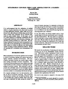
2) Formation Flying There are in general three types of satellite formations used in current missions. These are the following (as depicted in Figure 2.2): • Cluster Formations: A few satellites put in a dense formation to allow the fusing of satellite sensor data. These arrangements are used for interferometric observations, for creating high-resolution maps of Earth or for finding distant stars and planets.

Figure 2.2: The three types of formations: Example of a (a) cluster, (b) constellation and (c) trailing formation.


18

• Constellation Formations: Multiple, similarly equipped, satellites are (usually evenly) dispersed in a pattern to provide a wide area coverage. These are usually used for global communication and positioning networks. • Trailing Formations: Two or more satellites follow each other in the same orbit with only small separation. The satellites are usually equipped with different sensors and scientific instruments. This formation is used for high-resolution images and more insight into climatic trends in the Earth’s environment. The following are examples of previous and current formation flying satellite systems: The NMP/EO-1 (New Millennium Program - Earth Observation 1) mission was launched on November 21, 2000 as a technology mission designed to fly in a trailing formation with (60 seconds behind) NASA’s Landsat-7 as depicted in Figure 2.3. It autonomously maintains the separation within two seconds, using a controller, with an enhanced formation flying (EFF) algorithm, capable of autonomously planning, executing and calibrating satellite orbit maneuvres developed at NASA’s Goddard Space Flight Center (GSFC) (Folta et al., 1997). It allows for paired-scene comparisons with the images from Landsat-7. [Classification: SIZE-PAIR, COM-NONE, ARR-STATIC, CMP-HET, CTL-DEC]

Figure 2.3: Satellites LANDSAT-7 and EO-1 flying in a "trailing formation" Courtesy: NASA GSFC


19

The Earth Observing Sensorweb project developed uses the EO-1 satellite to obtain high resolution coverage of areas of interest. This system autonomously checks databases of alerts on volcanoes (MODVOLC) that are parsed from low resolution cameras on board of various satellites. Such alerts are then filtered and a change of the EO-1 orbit is requested automatically to allow for additional data. In short, it utilizes “low resolution, high coverage sensors to trigger observations by high resolution instruments" (Chien et al., 2005). [Classification: SIZE-LIM, COM-NONE, ARR-DYN, CMP-HET, CTL-CEN]

The Cluster mission, is a mission by ESA to study the effects of the solar wind around Earth in three dimensions. The mission, which was already designed in the early 90s but was delayed after the first four spacecraft were destroyed during launch in 1996, was the first space project that built craft in true series production. The four identical spacecraft, using a cluster formation (Figure 2.2a), started operation in February 2001 and will run until December 2009. Using identical instruments simultaneously, three-dimensional and time-varying phenomena in the magnetosphere can be studied. The satellites used their own on-board propulsion systems to reach the final operational orbit (between 19 000 and 119 000 kilometres) (Escoubet et al., 2001). [Classification: SIZE-LIM, COM-NONE, ARR-DYN, CMP-HOM, CTL-CEN]

The Afternoon (or "A-Train") satellite formation consists of seven satellites, as depicted in Figure 2.4, flying in formation (NASA, 2003). Currently five of the satellites are in orbit, two additional satellites, OCO and Glory, will join the constellation in 2009. The A-Train formation is designed to provide near simultaneous observations and continues study of aerosol distribution, cloud

Figure 2.4: The seven satellites of the A-train formation Courtesy: NASA JPL


20

layering, temperature, relative humidity, distribution of greenhouse gases and radiative fluxes. Its formation is maintained in orbit with a separation of only 15 minutes between the leading and trailing spacecraft with CloudSat and CALIPSO separated by only 10 to 15 seconds. The constellation has a nominal orbital altitude of 705 km and an inclination of 98 degrees. A more detailed description also of the seven satellites can be found in (Leitner, 2009). [Classification: SIZE-LIM, COM-NONE, ARR-STA, CMP-HET, CTL-CET]

The Galileo satellite constellation is currently being built by the European Union and ESA. It will use 30 spacecraft and is planned to be operational by 2013. The satellites send precise micro-wave signals with a time-stamp, allowing a receiver to calculate its position via triangulation. Similar are the Iridium and NAVSTAR (Global Positioning System (GPS)) satellite constellations, more information and examples can be found in (Leitner, 2009). Constellation formations are usually not flying autonomously and are groundcontrolled, therefore they are not considered autonomously cooperating robots. [Classification: SIZE-INF, COM-NONE, ARR-STATIC, CMP-HOM, CTL-CEN]

3) Rovers As mentioned before no missions with cooperating rovers are currently in operation or have been thoroughly planned. The closest to this is the current Mars Exploration Rovers (MER) mission, which put two identical rovers on Mars in 2003. These are though positioned quite far apart so no communication or coordination is possible. The software of the MER does include some behavior based control which allows for a more autonomous exploration (Huntsberger et al., 2000; Reeves and Snyder, 2005) and the possibility to add cooperative behaviors into future rover software.

Planned Missions and Visions Several space missions, where multiple mobile robots play a central role, are currently proposed. The research and funding of those areas has increased in the last years, mainly due to the above mentioned exploration visions announced by various space agencies (NASA, 2004; Visentin, 2008; Oda, 2008).


21

Many multi-satellite applications, especially in cooperation, are envisaged but very few are planned. The main focus in research is currently on optimizing formation flying (with respect to fuel usage) and on-orbit servicing, which might also help the development of in-orbit construction for larger structures. In the field of simulation, (Clark and Rock, 2003) proposed a trajectory/path planning technique based on dynamic networks, with simulation in 3D targeted especially for use with satellites. These systems are only in the very early development stage and do not provide optimizations of, for example, fuel consumption. For simulation and testing purposes the MIT has created a satellite testbed2 to verify planning and control algorithms experimentally. It allows for a 2D simulation of micro-gravity satellite control using air-bearings (Boning et al., 2008).

1) On-Orbit Servicing (OOS) On-orbit servicing is an increasingly interesting field in space applications. Some tests of servicing systems have already been performed, but those spacecraft usually have only passive cooperation, i.e. no direct communication between the servicing and the client craft is used. A European consortium of space companies proposed the HERMES OOS system. It is planned to use fuel from damaged, overloaded satellites as well as their fail-safe fuel at their end-of-life (EOL) and store the fuel on-orbit and use it to service other satellites. The system would consist of 5 different satellites in various sizes and specialized to do various tasks (Kosmas, 2007). [Classification: SIZE-LIM, COM-NEAR, ARR-DYN, CMP-HET, CNT-DEC]

JAXA is researching possible Hubble Space Telescope (HST) servicing missions based on their HII-Transfer Vehicle (HTV) spacecraft with added experience from the ETS-VII (see (Leitner, 2009)). The research concentrates on robotic servicing (capture/de-orbit). Future tests and operations are planned, for example, the Smartsat-1 mission, which tests automatic docking and orbital re-configuration of small satellites. The German Aerospace Center (DLR) started the DEOS (Deutsche Orbitale 2

Free-Flying Robot Testbed (FFRT)


22

Servicing Mission) project, which is based on the short-lived TECSATS (TEChnology SAtellite for demonstration and verification of Space systems) project and is currently awaiting Phase-A development. DEOS focuses on guidance and navigation and the capturing mechanism for non-cooperative as well as cooperative client satellites. While attached it will performing orbital maneuvres which can be used for de-orbiting of old, damaged or non-functioning satellites (Sommer et al., 2008). [Classification: SIZE-PAIR, COM-NONE, ARR-DYN, CMP-HET, CTL-CEN]

The main discussion right now seems to be whether a single platform servicing architecture or a fractioned servicing architecture will be the better choice. Most of the before mentioned, planned missions are currently on hold, under review or in an unknown state. A more thorough overview of the field of onorbit servicing can be found in (Tatsch et al., 2006).

2) Satellite Formations There are few satellites currently in orbit that are really cooperating, that means they use direct communication, arrange themselves to do tasks together or have some level of autonomously maintaining the formation. In academia there has been quite some research on optimization (Dumitriu et al., 2005; Nagai, 2009), decentralized control algorithms (Dumitriu et al., 2007) and autonomy (Martin et al., 2001), which increase the autonomy of the satellites and decrease the necessary control from the ground station.

Figure 2.5: The LISA spacecraft formation in orbit around the Sun. The spacecraft trail about 20 degrees (50 million km) after Earth. Courtesy: ESA


23

The Laser Interferometer Space Antenna (LISA) mission, a joint ESA-NASA mission depicted in Figure 2.5, will use 3 identical spacecrafts flying in a very large and widely dispersed formation, with 5 million kilometres separation between each other. This is the biggest formation to be flown yet. The main mission objective is to detect and observe gravitational waves from astronomical sources such as massive black holes and galactic binaries. One spacecraft is the dedicated master spacecraft and the only one contacting and sending data to Earth. The other crafts send their data to the ‘master spacecraft’ via a laser link. LISA is planned to launch in 2018. [Classification: SIZE-LIM, COM-INF, ARR-STATIC, CMP-HOM, CTL-CEN]

The DARPA System F6 (Future, Fast, Flexible, Fractionated, Free-Flying Spacecraft) project is currently in its early Preliminary Design Review (PDR) stage and planned for a launch in 2012. Papers (e.g. (Brown, 2007)) have been presented but none describe in detail the planned implementations. [Classification: SIZE-LIM, COM-NEAR, ARR-DYN, CMP-HET, CTL-HYB]

The idea of fractioned spacecraft was proposed by Molette in 1984. He claimed that the advantages would outweigh the higher mass and costs. A more recent presentation by BOEING comes to the same conclusion (Rooney, 2006). The MetNet project of the Finnish Meteorological Institute was started in 2000 and intends to land multiple probes on Mars to analyze the Martian atmosphere. These sensors spread on the surface are planned to communicate

Figure 2.6: The MetNet Lander (MNL) entry, descent and landing concept. Courtesy: Finnish Meteorological Institute


24

with the satellite in orbit which relays the data back to Earth. The precursor mission with the MetNet Lander (MNL) is planned to launch in 2011 (Harri et al., 2008). An illustration is seen in Figure 2.6. [Classification: SIZE-LIM, COM-NEAR, ARR-STATIC, CMP-MAR, CTL-CEN]

As can be seen from the projects and further papers, these multi-satellite systems are getting more autonomous and self-configuring, in the sense that these satellites can be launched by multiple launchers and different systems. After launch they are able to find their way into a given formation by themselves (Folta et al., 1997). ESA’s ACT is also actively investigating swarms of picosatellites for autonomous formations (Pinciroli et al., 2007). These will allow future satellite swarms to stay in formation autonomously and also to change their formations to best fit the mission objectives.

3) Space Structures Assembly JAXA plans to use robots to build space structures (in orbit and on the Moon) with the need for automatic rendezvous maneuvres, as well as construction of a space-based solar power system over the next 20 to 30 years. (Ishijima et al., 2005) present a control algorithm for tight cooperation between two robots to transport a beam in space. It presents ways to reduce the vibrations and reduce the fuel consumption of the robots. Space-based Solar Power (SBSP) or Space Solar Power Satellites (SSPS) are researched by JAXA as well as NASA, but not widely supported within those agencies, but JAXA has already tested a legged in-orbit construction manipulator in their laboratories on the ground and a schedule for a 1GW SSPS was proposed (Oda and Mori, 2003). The schedule plans to have small SSPS in operation by 2015 and the final satellite, constructed fully in space, by 2020.

Surface & Planetary Exploration The Mars Exploration Rovers (MER) are already in operation and although they do not cooperate (Reeves and Snyder, 2005) they show the future direction of (robotic) space exploration: rovers with more autonomy and larger systems


25

(i.e. multiple rovers). This section tries to shed a light on planned missions over the next decade and further visions of space exploration. The above mentioned possibilities for robots to be part of precursor missions for human space exploration are one of the main drivers in multi-robot (space) research. Since humans are more vulnerable to space conditions (e.g. radiation) and missions are planned to take longer than the current Space Shuttle missions, most of the proposed human space exploration missions for the next 2 decades include some form of human shelter (e.g. Martian or Lunar bases). Robotic teams are needed to investigate and prepare the landing site for the astronauts to follow (Schenker et al., 2003; Stroupe et al., 2006; Visentin, 2008). ESA is planning to use multi-robot teams in space exploration and included them in their ‘Visionary Outlook for R&D over the Next Decade’ (Visentin, 2008). One of the three main mission and research tracks from this outlook will be robotic agents, especially working in hostile and dangerous areas and acting in place of humans to perform assembly, maintenance and production tasks. They are especially trying to support the research and the possible applications of reconfigurable robot teams (Visentin, 2008): The aim is the development of heterogeneous, reconfigurable robots [...] to enhance the horizon of future mission regarding application areas, duration, and operational distance. These are planned to be tele-operated or operated semi-autonomously.

Examples Proposed topics for robotic space exploration include the mining of moons and asteroids, the construction of habitats, the detection of valuable resources (e.g. water or oxygen) and astronaut support during manned missions. A good overview can be found in (Baiden, 2008), though there is no focus on a multi-robot system. Rovers that are currently developed with a focus on space applications and use on Lunar or Mars surface are listed here.


26

The Robot Work Crew (RWC) at NASA’s Jet Propulsion Laboratory (JPL) was a project simulating the construction of planetary habitats by tightly coordinated robots (Schenker et al., 2003). A new robot architecture named CAMPOUT (see Section 4.2.3) was introduced and is still being improved and extended. The RWC consisted of two robots that together should complete a task used for building a structure. Another project (Stroupe et al., 2006) at JPL intends to follow-up the research done. [Classification: SIZE-PAIR, COM-INF, ARR-COOR, CMP-HET, CTL-DEC]

Developed at NASA’s JPL the LEMUR (Limbed Excursion Mechanical Utility Robots) (SIZE-ALONE) robots are designed to be easily reconfigurable and aim for application in space. Lemur 1 was designed for help with in-orbit construction, the current Lemur II can traverse very diverse terrains. They are though only single robots so far, no cooperation abilities have been added. The idea is to have multiple Lemur robots work together with a bigger (‘spider’) robot (see Figure 2.7) for construction and maintenance of satellites. [Classification: SIZE-LIM, ARR-DYN, COM-NEAR, CMP-MAR, CTL-CEN]

The paper presenting the cliff-descending AXEL robot (Nesnas et al., 2008), as well as other papers show that there is an increased need (from a scientific point-of-view) to provide the rovers with a higher mobility on rough terrains. Mumm et al.(Mumm et al., 2004) presented a system of 3 robots for these sit-

Figure 2.7: A marsupial system to inspect a solar array. Lemur robots with a larger Spider robot. (Stroupe et al., 2005)


27

uations. It uses 2 anchor robots to lower a third robot (attached by tethers), called a ‘rapeller’, down a cliff by cooperative action. The robots communicate via RF transceivers so that each robot has a complete knowledge of the system’s state. The anchors are aware of their positions and can control the tether. For cooperation, a behavior-based approach is used. [AXEL Classification: SIZE-LIM, COM-INF, ARR-COOR, CMP-MAR, CTL-CEN]

ESA has researched possibilities of data transmission and localization systems for simple drop-down microprobes, an advanced multi-robot system, showing the possibilities in the field of sensor networks. (Schiele et al., 2005). Competitions, such as the RoboCup and FIRA, allow for researchers to develop new techniques for team behavior and cooperation, which also support research in robot cooperation in future space systems. The rovers of the future are only envisaged, but according to the respective agency webpages no multi-robot missions with cooperation are funded either by NASA (the next rover missions are Mars Science Laboratory (2011) and a Mars sample return mission), ESA (trying to fly the ExoMars mission after various delays) or JAXA. This was also visible at the ‘10th ESA Workshop on Advanced Space Technologies for Robotics and Automation’ (ASTRA 2008) conference at the European Space Research and Technology Centre (ESTEC), where no multi-robot cooperation talks or papers were presented, as well as at the SpaceMaster Rover Symposium in April, where Dr. Volpe also mentioned the preference for single robot systems at JPL.

2.3 Coverage

2.3

28

Coverage

“Nothing is more difficult than the art of maneuvering for advantageous positions.” - Sun-Tzu

The coverage problem (sometimes also referred to as covering problem) is widely defined as to “cover a search space consistently and uniformly” (Menezes et al., 2007), or more informally stated, in the case of robotic exploration, to “see” every point of a given area, where “see” could be to move over it (and closely inspect it) or to have it in the field of view of a sensor. The area of research looking into problems of this sort is called computational geometry. The coverage problem for a team of robots was first mentioned in (Gage, 1992), which presented a categorization of the problem into three types: blanket coverage, barrier coverage, and sweeping coverage. Blanket coverage, which is the closest problem to the area coverage presented in this thesis, has the objective of maximizing the total covered area by a static arrangement. The coverage problem is known in many areas of research, also outside of robotics and touches on various interesting topics, for example: • area covering: how to cover an area completely and efficiently (Mazo and Johansson, 2004) • coverage path planning: optimal planning to the robots’ tracks to efficiently cover as much as possible of the area • wireless network coverage: how to place the base stations to increase coverage and reduce interference; a similar topic is sensor placement • grid coverage: in wireless sensor networks, which usually are assumed to be deployed in a grid layout, e.g. to provide surveillance • search and rescue problems: e.g. humanitarian de-mining (it has to find all the mines) and catastrophe victim search (where will the people most

2.3 Coverage

29

likely be); mathematical formalizations using defined spatial probabilities exist For research done in multi-robot coverage the problem can be interpreted as the “maneuvering of the robots into positions to keep the area constantly under good coverage with their sensors”. While there exist many papers covering a wide range of coverage problems, they mainly focus on area coverage in static cases, that is solving the problem of how to cover an area with hardly any changing conditions (apart from the robot movements), not much research has been done in more dynamic situations. The case of reacting to changing conditions, for example, a robot malfunction and therefore reduction of the team, or the change to a different target area, is quite important for this thesis and will be the focus of the research conducted. The following sections present the Art Gallery Problem a very well known and interesting problem in the area of complete coverage (which is interesting in, for example, astronaut support missions), the Boustrophedon Cellular Decomposition of areas, which is one way to split the area for multiple robots and finally an example of distributed coverage, which presents one possible way to cover an area as good as possible with multiple UAVs.

2.3 Coverage

2.3.1

30

Art Gallery Problem

A very prominent research topic is the Art Gallery Problem, which resembles the real-world problem of guarding an art gallery with a minimum number of guards (or video cameras), that can observe the whole gallery. The problem was first posed by Victor Klee in 1973 and proved to be difficult to solve for computers (NP-hard ) by (Aggarwal, 1984). Various alterations of the problem exist with a varying amount of boundary conditions and restrictions. An illustration of a typical Art Gallery Problem can be seen in Figure 2.8. In astronaut assistance this problem can be rephrased as ‘keeping all the astronauts in view with a minimal number of robots’.

2.3.2

Boustrophedon Cellular Decomposition

In (Choset and Pignon, 1997) an exact cellular decomposition approach for the complete coverage problem, called boustrophedon cellular decomposition, is presented. It solves it by splitting the area, and hence the task, into smaller

Figure 2.8: A typical Art Gallery Problem Courtesy: Claudio Rocchini

2.3 Coverage

31

cells that are ‘easy’ to cover. The path for a single robot is then computed by using the adjacency relationship of the cells. The name comes from the old English word boustrophedon meaning “the way of the ox”. It is used to describe the simple (robot) back-and-forth motion to cover an area. The terms used for this decomposition are (see Figure 2.9 for illustration): 1. slice, the area covered by the straight motion of the robot 2. cell, the decomposition of the area 3. critical point, the point at which an obstacle is first detected and the cell is split

2.3.3

Distributed Coverage Experiments

The field of distributed coverage with possible applications ranging from lawn mowing, to chemical and radioactive spill clean-up, and humanitarian demining is increasingly researched. A lot of this research currently focuses on how to optimize multi-robot systems for those applications. One way is to use the Boustrophedon Decomposition as a basis and apply it to multi-robot systems. Assuming global communication between the robots, the

Figure 2.9: Boustrophedon decomposition terms. Based on (Kong et al., 2006)

2.3 Coverage

32

cells are split up and each robot then plans its path in and between connected cells. This technique leads to decent results, as shown in (Kong et al., 2006), which allow for robust and complete coverage of an area with multiple robots. Another interesting approach is shown in (Schwager et al., 2009), where an optimal coverage for hovering robots is described. Their system uses a cost function, representing the fitness, to optimize the coverage of an area on the ground by multiple UAVs carrying downwards-facing cameras. The coverage is optimized by placing the vehicles in different positions and heights. The control of the robots is done autonomously with the help of an external vision system to gather the position information for every robot. Figure 2.10 shows the simulation result for ten UAVs.

Figure 2.10: Simulation results of 10 UAVs placed for optimal coverage. Courtesy: (Schwager et al., 2009)

Chapter 3 Problem Formulation “An undefined problem has an infinite number of solutions.” - Robert A. Humphrey

This chapter will start with a short overview of the problem and then go into the details of giving boundary conditions for this thesis work, emerging both from the systems used, as well as introduced to allow focusing on the main research problems.

3.1

Overview

The main focus of the research in this thesis is the problem of area coverage with multiple robots. The coverage problem was already described in Section 2.3. The aim of the thesis work is to find a placement for the robots, so that they cover as much of a given area with their sensors. This is similar to the definition of a blanket coverage, as used by (Gage, 1992). For this the robots have to be maneuvered into positions to keep the area (constantly) under good coverage. Another condition to satisfy is the optimization of the placement. This is discussed further down in Section 3.4

3.1 Overview

34

This thesis aims at using the marsupial robots, named Marsubots, developed and integrated here at TKK and shown in Figure 3.1. The system consists of one mother-ship and currently 6 smaller child robots. These are able to be stored inside the mother-ship and transported this way. The assumptions made are that the mother-ship is the main communication link to the operator or ground-station, it also provides the main energy supply, though the Marsubots are capable of intra-robot energy transfer. The work done here does not use the mother-ship but only the child robots to cover as much as possible of the target area specified. For future work, the other capabilities of this system can be used to further optimize the resource planning and sharing. The main research goal is to test a machine-learning based approach for area coverage using multiple robots. The algorithm should aim to optimize the coverage and minimize the overlap. Due to time and hardware constraints this thesis mainly performed simulation work and a simple implementation in another robot society (see Chapter 6). An interesting issue in this thesis is to provide good coverage also when the number of robots changes, due to, for example, hardware failure, communication loss or redistribution of the robot to another group and task. Autonomous control for moving the robots into a good formation in this dynamic environment is a goal.

Figure 3.1: The marsupial robot society at TKK

3.2 Boundary Conditions

3.2

35

Boundary Conditions

The boundary conditions, to limit the complexity and clearly define how the results were achieved, are mainly chosen to be close to the capabilities and limitations of the available robots at TKK. This thesis is designed to be implemented in a marsupial robot society, called Marsubots, depicted in Figure 3.1. The placement of the robots, and hence the coverage, is not considered a function of time, meaning that the area to be covered will not change. This is to ease the development of the robot control algorithms, especially the machine learning algorithm. One main assumption is the discretized area representation and with it the discrete coverage calculation. This restriction allows for faster testing and easier computation. It, however, limits the direct use of the simulation results in real-world experiments more than a continuous sensor model would. The robots will be controlled centrally, for example, from a mother-ship-type robot (or ground-control with satellites). This means that the algorithms do not need to be compatible with decentralized, autonomous robot control. Decentralization should though be kept in mind and, where possible, the control algorithms should be prepared for easy upgrading in the future.

3.2.1

Marsupial Robot Society

The TKK Marsubot society is a “novel multi-robot marsupial system for longterm autonomy” (Matusiak et al., 2008) with special focus on energy and versatility issues. Its specifications are listed in Table 3.1. The heterogeneous multirobot society consists of a marsupial mother-ship, named Motherbot, which provides extended functionality. For example, the mother-ship can transport the smaller robots, named Marsubots, in its ‘belly’ to otherwise inaccessible areas.


36

Marsubots The Marsubots are 3-wheeled robots, designed for autonomous indoor use, hosting a camera and LASER scanner as their main sensors. The two main wheels are 15 cm in diameter and coated with soft rubber, the third wheel, a castor, is used for stabilization. Currently 6 robots exist, with the lab aiming to build a total of 10 Marsubots. The robots are using two DC-motors for powering the wheels and two processors, a 16-bit microcontroller (PhyCore) for real-time control and sensor interfacing, and a Linux computer using an ARM9 processor operating at 400 or 600 Mhz, used for high-level controls, communications, camera control and machine vision algorithms. Emphasis was put on the power design to allow for long-term operations, therefore the robot can turn off all sensors and actuators, apart from the PhyCore processor, which is always powered on to monitor the energy state and recharging activities. The robot team communicates by sending messages via a wireless ad-hoc network. One main-feature is the ability of the Marsubots to transfer energy between them and also recharge at the Motherbot, this is shown in Figure 3.2. This allows for quite long operation times. (Matusiak et al., 2008) lists (theoretical) maximum operating times of 5.9 hrs while driving, 13.3 hrs when operated stationary and up to 81.0 hrs when in standby mode. Table 3.1: The robot specifications of the Marsubots robots at TKK. Robot Length/Width/Height

approx. 24/17/20cm

Axle Width

16.5cm

Main Wheel Diameter

15cm

Velocity, Acceleration

max. 20cm/s, max. 20cm/s2

Laser range

40.96cm, 240◦ field-of-view (FOV)

Camera planar FOV

around 45 − 55◦ (not calibrated)

Processor

a 16-bit micro-controller & a ARM9 Linux-box

Radio Link

AmbiCom WL1100-CP

Energy

3 Batteries á 2700 mAh, 1.2V Energy Transfer is possible.


37

Motherbot This is the mother-ship and by far the largest robot in the society. It is a tracked vehicle controlled by two motors. Three Marsubots can be carried by the Motherbot at the same time, while also allowing them to recharge their batteries, in its ‘belly’ located between its two tracks. The Marsubots can enter and exit via a deployable ramp. This docking, which is essential for recharging operations, can be done autonomously with the help of two tracks on the ramp. The current Motherbot is a prototype lacking some functionality, such as, for example, extensive sensors, some hardware and an aluminum hull.

System Size Regarding the coverage problem it is assumed that the Motherbot’s communications range and sensors cover as much area as the small robots, for the time being. For the simulation N robots are assumed, each having the size of a single cell in the (discrete) simulation. For more information and an introduction of these robots and also the current research see (Matusiak et al., 2008).

3.2.2

Robot Localization and Global Map

The robots are assumed to have the ability to localize themselves, i.e. the robots know where they are on a global map. Furthermore, it is assumed

Figure 3.2: Marsubots showing their ability to enter the mother-ship and dock for energy transfer.


38

that the robots know the environment, i.e. a map of obstacles exists, and no obstacles appear or change during the run, apart from the other robots. The robots therefore do not have to have a local obstacle avoidance algorithm, which eases the implementation of formation algorithms. The assumption is made, keeping in mind that in the case of a planetary area coverage application, the terrain and area are known, for example, through previous satellite scans. This condition though should be one of the first ones to be lifted and the system extended to support partly-unknown terrains, for example, new obstacles, not visible on the satellite scan(s), appearing during operations.

3.2.3

Terrain and Robot Motion

The terrain, due to the fact that a discrete simulation is chosen, is modeled using an occupancy grid. This binary grid represents the traversability of a cell by marking it occupied (true, 1, in the algorithmic implementation) for obstacles, or other robots. All the other cells in the grid are marked traversable or free (false, 0). This concept is extended to represent the terrain by extending it to multiple discrete layers. For easier use these layers are combined and a number denotes on which layer the obstacle resides. It is assumed that there is only one possible obstacle per cell and that the cell is also non-traversable on the layers beneath. With these assumptions the map can be represented as a grid, where each cell is described by a number in the interval [0, 9], 0 for no obstacle, h > 0 for an obstacle of height h, i.e. on layer h. The robots are assumed to be able to traverse cells having a height h that is in the interval ]hc − 3, hc + 3[, where hc is the height of the cell at the current position. Obstacles, therefore, have to be marked with a value which is outside of this interval, which is reasonable for the work done here but might be changed to a special obstacle representation in future projects and possible future versions of the simulator. The robots’ motion is reduced to some simple motions in the discrete grid, basically consisting of movements and rotations. The robot actions are shown


39

in Table 3.2. The actions MOVE RIGHT and MOVE LEFT were added to this list for simplicity reasons, those actions when executed at the robots are using a ROTATE-MOVE-ROTATE sequence. The motions can be executed in robotic experiments using a flat floor with uniform friction, confined by walls using elevation differences in discreet layers with ramps in between for traversing. Table 3.2: The simplified robots’ motion (grouped). Movement

Rotation

No Movement

MOVE FORWARD

ROTATE LEFT (CCW)

STAY PUT

MOVE BACKWARD

ROTATE RIGHT (CW)

MOVE RIGHT MOVE LEFT

3.2.4

Sensor Model

The sensor model to be used is another critical decision and important for this thesis. It is assumed that we have perfect sensors, i.e. no sensing error or noise in the defined sensor area. This is quite unrealistic in reality but reduces the complexity of the algorithm. This is another condition that limits the validity of the simulation in terms of real-world experiments, therefore also this should be lifted or changed to be more realistic as soon as is possible. The sensors can be modeled, not only as a 360◦ circular field-of-view (FOV) area, but also in elliptic form, as well as a cell-based form. In this a 2D coverage grid can be designed and added to each robot. Noise in the sensor and position information might be added, this is already taken into account and the system has a MakeDiscrete() function, which returns the cell the robot is in. A more detailed look at noise and other constraints of real world experiments should be performed in future projects. This thesis focuses on rover applications, but the term robots is used both for rovers and satellites, since the described problem can also be seen as a placement of satellites in the correct orbits for good coverage. The cost calculations and with it the optimization problem will though be quite different.

3.3 Multi-Robot Architecture

3.3

40

Multi-Robot Architecture

The laboratory at TKK is currently implementing a standardized architecture to be used with a wide range of systems, all using more than one robot. It is an auction based work- and task distribution system for the robots, based on the TraderBots approach described in Section 4.2.3. It will facilitate TKK’s own robot framework implementation called GIMNET (Saarinen et al., 2007). The simple task of Go_To_Pose, is being tested. For this each individual robot tries to calculate its cost to reach the given pose and makes a bid in the auction. The auction system is tested at a basic level, but the implementation of the motion commands in the robots has, due to issues with the embedded control and localization algorithms, not been tested yet.

3.4

Optimization Conditions

Related projects and papers show that various optimization criteria have been selected so far for similar problems. These range from simple ones, like measuring the time or counting the turns of the robots to more difficult ones like fuel-efficiency and schedule optimization. (Mazo and Johansson, 2004) measured the number of turns for the robots until the coverage was finished and then compared the algorithms by comparing these numbers together with the coverage percentage. In the case presented here, however, it is more interesting how much energy is needed to cover the area rather than how many turns (or how long) it takes. In a first attempt a single-feature optimization should be done using the number of actions necessary to create a good coverage or react to a change. A future option is to calculate the distance and energy needed for each action and optimize the energy use for the said problems. Another, future option will be a multi-feature optimization, which could be implemented as an extension to the machine learning algorithm.

3.5 Mathematical Formulation of the Coverage Problem

41

Another interesting optimization criteria, in the future, could be the complexity of the used algorithm. This might be quite interesting due to the limited computational power on space-proof embedded systems.

3.5

Mathematical Formulation of the Coverage Problem “It is a mistake to think you can solve any major problems just with potatoes.” - Douglas Adams

This section will try to look more closely on the mathematical issues involved in the coverage problem. The problem as stated before is widely defined as to “cover a search space consistently and uniformly” (Menezes et al., 2007). Mathematically the coverage calculations do not differ, whether one or multiple robots are used. This is based on the fact that even a single robot covers only one area at a given time step. The main question is “How much of the area can be covered in n time steps?”, this means what is the full area of the n separate covered areas. This question can be rephrased, how much area do n robots cover at a give time step, which leads to the same mathematical formulation. A simple formulation of the coverage problem is given in (Mazo and Johansson, 2004), where a rectangular target area is defined as Ω = [0, L] × [0, W ] ⊂ R2 ,

L, W > 0

(3.1)

The covered area Ψ, is rather complex to define due to the fact that, in the general case, Ψ is a union of sets (polygons in geometry). The calculation of such is, using the well-known Inclusion-Exclusion formula, defined as A

∪ni=1

pi =

n X i=1

+

A(pi ) −

X

A(pi 1 ∩ pi 2 ) + · · ·

(i1 ,i2 ):1≤i1 DirectionTo(rB->GetPosX(), rB->GetPosY());

rA->AddVector(power * scale, dir); // repulsive force due to sensor if(calculateRepulsiveForces) { scale *= CVectorBasedMover::SCALING_FACTOR; power = rA->GetSensorArea()->GetDistanceInDirection(dir); rA->AddVector(power * scale * -1, dir); }

4.4 Placement Using Machine Learning

57

In the listing a SCALING_FACTOR variable can be seen, which is added to generate more sensible results. More information about it can be found in Section 6.2.1. The CVectorRobot class is extending the CRobot class and provides functions to add and sum force vectors to the robots. These vectors are using a structure defined in Listing E.7.

4.4

Placement Using Machine Learning

The algorithm presented here uses machine learning (ML) techniques to calculate the optimal placement of the robots for area coverage. For this the works of Prof. Takadama are used and built upon. The algorithm uses an organizational-learning oriented classifier system (OCS) as the basis for its implementation, therefore using a combination of reinforcement learning with a genetic algorithm to find suitable actions for the multi-agent system. It has a very similar structure to the algorithm presented in Section 4.2.1. The ML approach tries to optimize the solution by checking validity and fitness of solutions for the given search space, that means that the machine learning is used for searching for the best solution. The OCS system consists of autonomous agents, which all have their own LCSbased implementation but feature the same architecture. Each agent is able to recognize the environment and its local state, done in the Detector() function, and is able to change the environment due to a chosen action, implemented in the Effector() function. The COCSMover class is the main implementation of the learning algorithm and facilitates an object-orientated approach for representation of the agents and the environment. Figure C.3 depicts the classes used and their relations, whereas the architecture, which is based on the OCS, can be seen in Figure 4.3. Each agent has its local memory, which is used to create, store and update rules, also called classifiers (CFs). These rules are used to select the most suitable action for the current state. The memory is split into Organizational Knowledge Memory, Individual Knowledge Memory, Working Memory and a Rule Sequence Memory. The agents then also include


58

the learning functionalities and techniques. Including reinforcement learning, organizational knowledge reuse, rule generation as well as the GA technique for rule exchange. The agents, having both a local objective function and local rule-set, detect the environment state and decide the action based on the state. In this cycle each agent updates its own rule-set. The OCS system tries to focus on emergent processes, in which the agents form dynamically groups with autonomously generated adaptive behaviors. This means that agents, though having their own adaptive rule-sets, exchange rules at given crossover times.

4.4.1

Pseudo-Code

The code here should give an overview of the implemented algorithm and its main components, while skipping programming language specific details. The main OCS function is shown in Listing 4.2. Listing 4.2: The OCS algorithm procedure OCS iteration := 0 Collective_Knowledge_Reuse while iteration < MAX_ITERATION reset the problem to the starting position iteration := iteration + 1, step := 0 while not solution_converges Detector() Rule_Generation, Rule_Exchange Effector() step := step + 1 end Reinforcement_Learning, Collective_Knowledge_Reuse end end


59

Listing 4.3: Collective_Knowledge_Reuse procedure procedure Collective_Knowledge_Reuse if iteration = 0 used stored collective knowledge else if solution is the best if collective knowledge is set already delete stored collective knowledge store current rule-sets as collective knowledge end

The collective knowledge is used to save role specialization and allows for reuse of good solutions in future problem solving. It is also called organizational knowledge since it works as as “organizational double-loop learning” (Takadama et al., 1999). This mechanism, as described in in Listing 4.3, reduces the learning count and is needed when no solutions can be found without organizational knowledge.

Listing 4.4: Rule_Generation procedure procedure Rule_Generation for all agents if no classifier matched if number of classifiers = MAX_CF delete CF with lowest strength create a new CF set strength to initial value end end

The Rule_Generation procedure, as shown in Listing 4.4, has the main use of creating new classifiers, when no classifiers in the current rule-set, i.e. the Individual Knowledge Memory, match the current environmental state. This means that the Detector() function did not leave a classifier in the working memory of the agent. If the maximum number of classifiers in the Individual Knowledge Memory is reached the weakest rule is dropped to make space for a new CF.


60

Listing 4.5: Rule_Exchange procedure procedure Rule_Exchange if mod(step, CROSSOVER_STEP) = 0 for a random pair of agents order rules by strength for the weakest CROSSOVER_NUM CFs if strength < BORDER_ST delete CF copy CROSSOVER_NUM strongest from other agent reset strength to START_STRENGTH end

The CFs between agents are exchanged, similar as in the Pittsburgh LCS approach, at every crossover operation, as shown in Listing 4.5. The rules are replaced by the best CFs of a randomly chosen, i.e. non-elite selection, of counterpart, unlike in conventional evolutionary computing, where elitist offsprings are created, i.e. the best agents are used to create new agents from their ‘genome’.

Listing 4.6: Reinforcement_Learning procedure procedure Reinforcement_Learning if solution_converges for all agents for all fired classifiers strength is updated according to the reward end

The Reinforcement_Learning procedure, as shown in Listing 4.6, updates the strength of each classifier in the Rule Sequence Memory in the case of a converging result. In that case the fired CFs, all the CFs in the Rule Sequence Memory, get a reward, how the reward is spread is described further down.


4.4.2

61

Classifier

The rules in each agent are created and removed as in the Michigan-LCS case. This means that new CFs are created when a new environment state is detected, and deleted when a certain amount of CFs already exist in the local rule-set. The classifiers are the same as the rules in LCS, simple if-then constructs composed of three parts: (i) the condition, (ii) the action and (iii) the strength or fitness value. The condition, or if clause, of the CF contains various information about the environmental state. It usually consists of multiples parts including the last action done and other input information. The action, or then part, defines the action to be executed by the agent if the condition part matches the current environment. The third part, the strength value, defines how good the CF is, which affects selection and therefore the agent’s behavior.

Condition The condition part of a classifier is representing the knowledge of the current situation. It is a list of input values, represented by the ternary

Listing (4.7): Code for the CFs enum eCFCondElements { PREV_ACTION = 0, OVERLAP, LOC_CHANGE, PREV_CONDITION }; //... char cond[CDPARNR]={’#’,’#’,’#’,’#’}; // init others cond[PREV_CONDITION] = prevOverlap - ’0’ + cond[OVERLAP]; if(cond[PREV_CONDITION] != ’0’ && cond[LOC_CHANGE] == ’1’) cond[PREV_CONDITION]++; prevOverlap = cond[OVERLAP];

Figure 4.6: The structure of the rules, also referred to as classifiers (CFs), used in the OCS implementation. based on (Takadama et al., 1999)


62

alphabet {0, 1, #}, though extended in some cases. Figure 4.6 shows the structure of the CFs and the condition in the OCS algorithm based on (Takadama et al., 2002). It also shows the code for the enumeration and the initial CF. The elements of the condition are defined in the eCFCondElements enumeration and are the following:

1. An indiction of the previous action done by this agent (PREV_ACTION). For the first condition this field is #. (Any character representing an action.) 2. A flag representing an existing OVERLAP of this agent’s sensor area with another agent. (0 or 1) 3. A flag representing a location change based on the last action chosen (LOC_CHANGE). (0 or 1) 4. A field indicating the previous condition (PREV_CONDITION) of the environment. This is calculated in the Detector() function. (0-3)

Actions The actions of the agents are the same as described in Table 3.2 (Section 3.2.3). The 7 actions are represented by a character and are defined in the eAgentAction enumeration, see Listing E.6.

4.4.3

Memories, Mechanisms and the Environment Model

Memories are needed for learning, it stores various information about the classifiers at each agent. In the memory CFs can be created, stored and updated. The memory each agent can access is split into four parts, as introduced by (Takadama et al., 2002): (i) Organizational (or Collective) Knowledge, (ii) Individual Knowledge, (iii) Working and (iv) Rule Sequence memory.

Organizational Knowledge Memory Also referred to as Collective Knowledge Memory, this memory stores a a global set of the various rule-sets at each


63

agent. This knowledge is shared by all agents and allows for role specialization and classifier reuse. The mechanism, with more information on the collective memory, is described in the next sub-section.

Individual Knowledge Memory This memory stores the current rule-set of every agent. This is where the knowledge of the individual agent is developed over the various iterations. At first FIRST_CF number of rules are generated and initialized, then during the learning operation new rules are added or exchanged with other agents. There are always at most MAX_CF classifiers stored in every agent’s rule-set.

Working Memory For operations in the agents, e.g. selection of matching CFs (i.e. creating of the match-set [M]), a temporary list (in the implementation a std::list pointer) is available to be filled with CFs. At the end of the Detector() function it will be filled with the match-set, whereas before calling the Effector() function the selected and to-be-fired rule should be placed in here.

Rule Sequence Memory The fired rules are stored in this memory in chronological order. The received reward is then spread on all the CFs in this sequence.

The OCS algorithm has four separate forms of learning mechanisms implemented. These are taken from evolutionary computing (and genetic algorithms) as well as from organizational learning techniques and were already presented above in pseudo-code.

Collective Knowledge Reuse The reuse of good solutions in future problem solving is helping in reducing the learning as well as solving problems that need this organizational knowledge. This name is derived from its central set of agent behaviors, as is depicted in Figure 4.7a. This is not yet implemented


64

in the current OCS learning mechanism, due to debugging reasons and time constraints.

Rule Generation As the name suggests, rule generation is used to create new classifiers. This operation is performed when no CFs in the rule-set of an agent, i.e. the Individual Knowledge Memory, match the current subenvironment state the agent detects. The generation of new CFs allows to explore other solutions to the problem, that have not yet been tested. These new CFs are created, in the agent’s GenerateRule() function, with a random action value and a condition based on the state detected in the Detector() function. The strength is initialized with the START_STRENGTH constant. If there already exist MAX_CF number of CFs in the rule-set of this agent, the weakest rule is to be deleted before the new one is created. The rule generation is depicted in Figure 4.7b.

Rule Exchange The rule exchange mechanism is used to generate an exchange of rules between two agents. This crossover operation, as it is called in genetic algorithms, generates new behaviors in the agents and explores therefore, like the rule generation mechanism, new ares and CF combinations. The CFs of two, randomly chosen, agents are exchanged, at every CROSSOVER_STEP. The rules are sorted by strength and the CROSSOVER_NUM weakest are replaced with the strongest of the other agent. Here this rule exchange differs from conventional crossovers, where usually elitist offsprings are created. The strength values of the rules introduced from the other agents are then reset to the starting values, since effective rules in one agent do not necessarily have to be effective in another in multi-agent environments. The rule exchange is depicted in Figure 4.7c and the code is presented in Listing E.2.

Reinforcement Learning (RL) A reward received for a converging solution is spread over each classifier chosen. These are stored in the Rule Sequence Memory and the spreading is based on the following exponential function ST (i) = ST (i) + R × Gn−i

(4.3)


65

where i = 1, 2, ..., n, n being the number of fired CFs, ST (i) is representing the strength of the i-th CF, G is a geometric ratio (usually 0.8 or 0.5) and R the full reward received, as presented in (Takadama et al., 1999). A function graph is shown in Figure 4.7d. This spreading is done at every agent in its respective SpreadReward() function, see Listing E.1.

The environment interactions are modeled in the CEnvironment class and are used from the agents in the following two functions for retrieving the current state (Detector()) and react to it by executing an action (Effector()).

Detector() This function is run at every time-step at every agent and detects the current state of the (sub-)environment. The main objective of this function is to create a new condition that represents the state and put it into the working

(a) Collective Knowledge Reuse

(b) Rule Generation

(c) Rule Exchange

(d) Reward Spreading in RL

Figure 4.7: Illustration of the four Learning Mechanisms used in the OCS algorithm. Courtesy: (Takadama et al., 2002)


66

memory of the agent. From this condition later the match-set will be created. In a way this means that it models the environment into a 4-field vector for the agent, as described above. Firstly the previous action (PREV_ACTION) is retrieved, or set to # if it is the first step. Secondly it checks for overlaps (OVERLAP) of the current agent’s sensor area with other agents, this is done via the RobotCoverageOverlaps() function of the Model (inherited from the CEnvironment). Thirdly the location change (LOC_CHANGE) flag is set if the location changed, based on the chosen action and also a last-location memory. Lastly, the previous condition (PREV_CONDITION) is calculated by adding the last iterations overlap together with the current. If one of them is set, also the value of the current LOC_CHANGE flag is added. For simplification the creation of the match-set is already done here.

Effector() The action chosen by the algorithm for every time-step is put into the working memory. This function then just checks the CFs for the retrieving the action and returns the action. In the COCSMover class, with the help of the Model class, the robot is given the action to execute it.

4.4.4

The COCSMover Class

The COCSMover class encapsulates the OCS learning and also allows it to be used as a formation control algorithm in the simulator, due to being derived from CRobotController. The simulator acts as the feedback for the environment, shows a visualization and allows for some easier control, for example pause/continue the execution. Inside the class the real machine learning happens, this could in future versions be moved into an external class to separate it from the robot control (simulator) functionalities. The learning starts in the RunController() function, which saves the initial robot positions to allow to return to the starting problem at every iteration. As a first step of the algorithm the Detector() functions at every robot are called to create the match-set, from which one CF

4.5 Optimization

67

is then selected in the LocalEvaluationFunction(). This is done using a roulette-based selection process, in which each CFs probability of selection is based on its strength relative to the sum of all match-set CF strengths. After retrieving the action via the Effector() the action is also done in the simulator. Every CROSSOVER_TIME step the rule exchange is done and after every iteration, that means, after the result converges, the reinforcement learning is done, where both mechanisms work as described above.

4.5

Optimization

The problem described here is a so called NP-hard problem, it is hard to calculate the optimal placement, but it is simple to check the fitness of a solution (how optimal the solution is). These problems are often applying evolutionary computing to find better solutions. In this case here the placement is optimized for one single feature. This so called single-feature optimization is in area coverage usually chosen to be the covered (target) area. Other options here could be the calculation single robot coverage or optimal formation placement. Both algorithms, when implemented to just focus on the coverage of the target area, lead to good results, which are presented and compared in more detail in Chapter 6. Currently the OCS algorithm defines the fitness function the following way: • If there exists some coverage of the target ares the yielded reward rc is: rc = MIN_REWARD + (MAX_REWARD − MIN_REWARD) × Cov • If no coverage exists: the reduction of the distance to the target area is used to calculate (a smaller) reward rd , based on the following equation rd = MIN_REWARD ∗ .8d , where d is the distance to the target (divided by 250).

4.6 Changes in Formation

68

Multi-Feature Optimization Better results, meaning an optimization of multiple criteria, can be done with so called multi-feature optimization. Some genetic algorithms have been proposed to solve these problems. An overview can be found in (Deb and Kalyanmoy, 2001).

4.6

Changes in Formation

Apart from the placement problem discussed above, another interesting issue is the change of formation due to changing conditions. Some thoughts about possible extensions for the approaches to tackle this problem. Because of the limited time and increasing complexity this problem was though not solved in this thesis. One idea was to extend the machine learning (ML) approach to be able to handle these situations. This could be done by adding another algorithm, that works with the results of the OCS learning algorithm presented here and uses the optimal configurations found to generate a transition matrix. This matrix would contain which formation to switch to, according to some optimizing criteria, if one robot fails. Most likely it would contain different results depending on which robot fails. The implementation of this was harder than expected, therefore no changes were done in the COCSMover class for the case of robot failures.

4.7 Coverage Calculation Math

4.7

69

Coverage Calculation Math

“If people do not believe that mathematics is simple, it is only because they do not realize how complicated life is.” - John Louis von Neumann

In this thesis a discrete coverage representation is used and mathematically defined as described in Section 3.5. The CDiscreteCoverageCalculator class implements this. Due to its simplicity just a few lines of code are needed for implementation, as seen in Listing 4.8. Listing 4.8: The CalculateCoveredArea() function, counting the covered and target cells. for(int j = 0; j < rows;j++) for(int i = 0; i < cols;i++) { int x = i*CELL_WIDTH + CELL_WIDTH*.5; int y = CELL_HEIGHT*.5 + j*CELL_HEIGHT; if(targetArea->InArea(x, y)) { targetArea++; if(robots && robots->Cover(x, y)) coveredTargetArea++; } }

The coverage is then simple given by Cov =

coveredT argetArea targetArea

(4.4)

A version of a continuous coverage calculation would work with only circles at the beginning, and then extend to work with polygons. It should be noted though that the calculations get complex rather quick. The application of one such approach is presented in (Schwager et al., 2009).

Chapter 5 Simulator “Have you ever had a dream, Neo, that you were so sure was real? What if you were unable to wake from that dream? How would you know the difference between the dream world and the real world?” - Morpheus, The Matrix

This chapter describes the implemented simulator, which is designed to ease the development of the formation algorithms before finalizing and testing them on the robots. It shows its internal structure, as well as how it is implemented and used in connection with the algorithms described above. Its implementation started during the three months at the ISSL of the University of Tokyo, when the main parts were also finished. Extensions development and code debugging was done throughout the whole project.

5.1

Overview

To test the algorithms described in Chapter 4, a specific simulator was implemented. This was done after checking and testing of available simulators in the labs at TKK, as well as at ISSL. The simulators currently in use at ISSL are mainly for dynamics and attitude control of satellites. Though this thesis

5.1 Overview

71

work is also applicable to satellites, those simulators do not provide information about the field of view of the sensors on-board, which is necessary to calculate the coverage area. At TKK various simulators have been implemented in the past but these are generally used for very specific problems and projects. There have been efforts to utilize those simulators in other projects and start a merging of technologies and knowledge but, since they are very specific and not designed to be general, it was decided to develop another one for illustrating multi-robot cooperation for the coverage problem. Development of the simulator for multi-robot control (SMRTCTRL) started in February 2009. Its aim is to have a simple simulation capability to visualize the output of the control algorithms. It shows a 2D, birds-eye view of the operating area, visualizing the terrain, which can be loaded from a simple digital elevation map (DEM), and displaying the robots deployed there. The simulator uses a discrete representation of the scene, this being the current standard for coverage simulators (see e.g. (Zheng et al., 2005)). It visualizes the sensing area of each robot based on heading and position and changes it according to the terrain. The simulator, implemented in C++, tries to follow common usability and user control guidelines. It uses SDL as main visualization library, its advantage of being platform independent comes with the disadvantage of not having a simple graphical user interface (GUI) components library. To overcome this, a lightweight library, named liglui, was developed and released to the public (see Appendix B). Using C++ also allows for object-oriented development, as for example seen in the abstraction of the robots and their sensing areas. To sum up, the main features of the SMRTCTRL simulator are: • 2D birds-eye view • discrete representation • visualization of sensing and target area • user-friendly GUI • platform-independent and object-oriented implementation

5.1 Overview

72

The aim of the simulator is to provide an easy way of testing various multi-robot control approaches, the system is general enough to provide feasible simulation of the results of various formation control algorithms, it can also be used to test other components of a multi-robot system, like path planning, task sharing or simply multi-agent architectures. An alpha version, dubbed Aurora was presented at the end of March. It was the first draft version, already spotting the user interface and a simple version of the user controls. For the seminar presentation, as well as the presentation about the work progress in Tokyo, a beta version, dubbed Borealis was released by April 20. A screenshot can be seen in Figure 5.1. The main improvements over the first version are the added abstractions for the formation control classes and testing with a simple algorithm. The third version, nicknamed Corona, was released in time for the review presentation in mid-June. It added the terrain/sensing area interactions, i.e. changing of the sensing area based on the DEM, as well as sanity checks for the robot movements.

Figure 5.1: A screenshot of the Simulator’s Borealis release. The figure was taken from a presentation and indicates some of the features.

5.2 Internal Design

5.2

73

Internal Design

The SMRTCTRL simulator was created as a by-product of the main research work of this thesis. Its internal structure is described in detail in Appendix D, where it explains the paradigms used, the architectures implemented, as well as the interactions and connections of the subsystems. Appendix C, is also of interest since it includes the connections to the simulator. The simulator is based on the very common architectural approach in software engineering, called Model-View-Controller (MVC). MVC helps by separating the graphical user interface (GUI) (view ), the business logic (controller ) and the data representation (model ).

These separate entities are running

in their own threads, as the simulator is able to run multi-threaded, with a platform-independent thread implementation provided by the SDL library (see Section D.2). The code is also separated due to the object-oriented approach available with the C++ programming language. This allows not just for encapsulation but also for easier code reuse and extendability in the future.

5.3

Discrete vs. Continuous Simulation

A discrete representation was chosen for this simulator, to allow for simpler simulation, especially of high-level control algorithms. This is backed by the fact that these algorithms usually leave all the low-level sensor and control problems out of their scope. In related work, for example (Zheng et al., 2005), coverage simulation is mainly done with a discretized scene. There exist various approaches on how to discretize the environment. SMRTCTRL uses a simple quadratic cell decomposition of the continuous scene for calculations but allows for continuous visualization, see Figure 5.2. The issue on how to be able to use simulation results on real robots is of interest to lots of researchers in this field, it is also the main topic of a workshop at the 2009 Robotics: Science and Systems Conference, “RSS 2009 Workshop

5.4 Visualization

74

on bridging the gap between high-level discrete representations and low-level continuous behaviors” 1 . Other approaches using discrete representation include, for example, (Beni, 1988) describing a multi-robot cooperation system with robot interactions only possible at the corners of pre-defined cells. The data model provides a MakeDiscrete() function that allows the calculation of discrete (cell) values based on the settings of CELL_WIDTH and CELL_HEIGHT, see Listing E.9. These calculations are done based on (planar) Euclidean distance calculations, where the distance of two points in an p 2D plane is defined as ∆x2 + ∆y 2 , or alternately based on Manhattan distance calculations, where the distance is defined as simply ∆x + ∆y. For these calculations a class CCalc was implemented, see Listing E.3.

5.4

Visualization

The main feature of the simulator is the visual output provided from the robot formation control algorithms. This is done with the Simple DirectMedia Layer 1

http://learning-robots.de/TC/RSS2009

(a) Discrete visualization

(b) Continuous visualization

Figure 5.2: The visualization difference between discrete (using Euclidean distance) and continuous representation.

5.4 Visualization

75

(SDL) library, which provides a widely used, Open Source, cross-platform interface, written in C and supporting C++ natively. It also has bindings to a great variety of other languages and can be downloaded freely from the project’s homepage2 . The GUI class handles all the visualization, by encapsulating most of the GUI components functionalities in the CGUIObject class, taken from the liglui library. The DrawGUI() function, which can be seen in Listing 5.1, is the main drawing function for the simulator. Listing 5.1: DrawGUI(), drawing the whole simulator’s user interface. void GUI::DrawGUI() { SDL_FillRect(screen, NULL, 0x888888); // Draw Background // Draw Terrain if(chkShowTerrain->GetStatus() && model->GetTerrain()) model->GetTerrain()->Draw(screen); // Draw Grid if(model->IsDiscrete()) DrawGrid(); // Draw Robots if(model->GetRobots()) model->GetRobots()->Draw(screen, model->IsDiscrete(), chkShowRobots->GetStatus(), chkShowVectors->GetStatus()); // Draw Target Area if(model->IsTargetAreaVisible() && model->GetTargetArea()) model->GetTargetArea()->Draw(screen, model->IsDiscrete()); // Draw Dashboard & UI if(dash) dash->Draw(screen); // Update Screen SDL_Flip(screen); } 2

Simple DirectMedia Layer (SDL) Webpage: http://www.libsdl.org/

5.4 Visualization

76

The visualization of the robots’ positions is done using the robots’ IDs, as well as marking the cell in blue. More details about the actually drawing of the sensing area, as well as, the robots can be found in Section D.2.

Terrain and Grid Drawing The terrain is the first to be drawn on top of the blank background surface. As already mentioned in Section 3.2.3 it is based on a discrete occupancy grid. This is then visualized as seen in Figure 5.3. If the current visualization is supposed to be discrete, which can be set by a checkbox in the GUI, a grid is drawn over this terrain. It consists of single-pixel-wide lines in a light green colour, which are spread by CELL_WIDTH (horizontally) and CELL_HEIGHT (vertically) constants, with a default value of 20px for both.

Terrain and Sensing Area Interaction To allow for the terrain to interact with the robot sensing area, i.e. changing the sensing area based on the terrain, other functionality was introduced. These include the CCellBasedTargetArea class, featuring its CheckArea() function, which will be called by each robot after it was moved or rotated. The representation of the sensing area was changed to be using a similar occupancy grid as the terrain. A 2D grid around the robot is produced, which binary encodes whether the robot sensing area covers a given cell. After this

Figure 5.3: The terrain visualization in the SMRTCTRL simulator.

5.4 Visualization

77

2D grid is initialized it is copied into the active, working memory of the sensing area. After every move of the robot, and hence the sensing area, firstly the initial sensing area is copied over the active one, and secondly tested for terrain interactions. The terrain interactions are the following (this is also the order in which they are checked in the code): • Extend Sensor Range based on current ‘altitude’ of the robot, which is basically the height information from the terrain. • Reduce Coverage Around Obstacles that are within the sensor range, i.e. terrain elevations different from the robot’s. For more detailed information about these interactions and how they are implemented consult Appendix D.2.

Dashboard A special case is the Dashboard, it allows for simpler user interaction, by providing a space for buttons, checkboxes and switchboxes, which allow for selecting one of multiple options. The options range from switching the control algorithm to different visualizations. The code for the sidebar was developed during this thesis and is available in the liglui project. More information about the liglui library and project can be found in Appendix B.

Chapter 6 Results “In theory, there is no difference between theory and practice. But in practice, there is.” - Yogi Berra

6.1

Standard Initial Configuration

For better comparison between the algorithms a standard initial configuration was used. This configuration reflects a marsupial society just deployed, i.e. the child robots have just disembarked from the mother-ship, with the target area set in medium distance. The terrain is consists of different elevations representing a crater-like environment. The initial configuration is using: a mother-ship (Motherbot), which is, for these two control algorithms, not moveable and has a circular coverage area (5x5, 25 cells), as well as four controllable child-bots (Marsubots), each possessing an elliptic coverage area (5x7, 27 cells). These sport an initial formation with a gap of one cell in between the robots. The target area is defined as a circular area, 69 (9x9) cells in size, and placed 22 and 11 cells away in X and Y axis respectively. The terrain used can be seen in Figure 5.1.

6.2 Robot Placement

6.2 6.2.1

79

Robot Placement Vector-Based Simulation Results

Starting with the before-mentioned initial configuration the robot control algorithm starts moving the robots based on the calculated force vectors. The system leads to a converging coverage in most cases, though in some situations a singularity (robots are all together moving in one direction, away from the target) or oscillations (robots start moving back and forth) are observed. The simulation of the robots was done, as described in Chapter 3, where the robots are described to have seven possible actions to perform. The vector-based control approach was mainly aimed to be tested with circular target areas and therefore does not implement a directional force vector, hence the robot actions are reduce to the four motions (forward, backward, left, right). For the simulation runs no obstacles were inserted and no terrain interaction was performed on the sensing areas. The simulation also assumed that all actions can be completed within one time step or tick and that the robots can be controlled simultaneous, which turned out to be difficult during the SMURFS project (see Section 6.3). The vector approach was mainly tested using circular sensing areas, when switched to elliptical too much repulsive force is generated, due to the lack of a directional understanding, and hence not a full coverage can be found. This tests, with the elliptic sensor areas, showed that the algorithm converges to a stable formation after 83 actions, generating a combined coverage of only 12%, or 8 of the 69 target area cells. This could be overcome by using a more thorough selection of the scaling factor and include a directional component. An interesting effect observed was that robots with smaller sensing areas are moving closer to the target, and by doing so, drive the robots with larger areas away from it. This is explained by the target force calculation, which leads to larger forces in the direction of the target for robots with smaller coverage (since there is a smaller repulsive force).

6.2 Robot Placement

80

Scaling of the Repulsive Forces As already mentioned in Section 6.4, a scaling factor, referred to as λ, was added to the repulsive forces to allow for better coverage and less interference. This factor was set to 1.2, since it was observed to be the most suitable value in simple simulations using circular sensing areas. The data, i.e. different values for λ, together with a screenshot of the simulator can be seen in Table 6.1. The coverage column represents the coverage reached by four robots using circular sensing areas and the respective λ value in the force calculation of the CVectorBasedMover class. It can be seen that the algorithm performs better with circular sensing areas than with elliptic sensing areas, which only reach a coverage of around 12%. In this case the terrain was ignored for the robots’ movements as well as their sensing areas, this was done to put emphasis on the scaling factors to be chosen.

λ

Coverage

0.8

97%

1.0

100%

1.2

100%

1.4

100%

1.6

93%

2.0

83%

(a) λ scaling factors

(b) Simulated result for λ = 1.2.

Table 6.1: The scaling factors used in the vector-based simulation, using circular sensing ares, together with the resulting coverage and an image of the result yielded for λ = 1.2.

6.2 Robot Placement

6.2.2

81

Machine Learning Simulation Results

The initial configuration mentioned above, is used as the starting configuration for all ML algorithm test runs. The COCSMover class uses the classifier-action pairs selected through learning in every iteration to control the robots’ motions. After a convergence in the result of one population, the robots are reset to their starting positions and another learning iteration is done. Figure 6.1 shows the evolution of one representative result using the OCS approach. Throughout the iterations the agents and therefore the global solutions are increasingly optimizing the coverage problem, with the the best coverage a bit over 26%, which is better than the vector-based approach. The dots are the coverage at each iteration steps with the best coverage connected by the dashed line. It can be seen that the results are varying quite a bit but an overall trend to increased coverage is visible. The crosshairs represent the summed distance of all robots to the target, which is the second fitness criteria, at each iteration. The solid line represents the closest distance found in the all the iterations so far. It does not always correlate with the best coverage, though here the best coverage solution has also a close to optimal distance. The figure shows that the randomized, learning approach does overall yield a good coverage with a good distance and that the best solution improves over time. The test run used the following settings for its OCS learning to obtain the result: Each agent has between 15 (at start, FIRST_CF) and 30 (MAX_CF) classifiers and exchanges 7 at every crossover step (CROSSOVER_CF_NUM). These classifiers are initialized with a strength of 1.0 (START_STRENGTH) and the border strength (for crossover) is set to 1.15 (BORDER_ST). The test run had a maximum number for 500 iterations (MAX_ITERATIONS), each with a maximum of 300 steps (MAX_STEPS), but the average number of steps per iteration was only 68.3. A rule exchange between two random agents was done every 10 steps (CROSSOVER_STEP). The average reward per iteration was only 1.86 (with the maximum at 6.3). As with the vector-based approach for the simulation no obstacles were inserted

6.2 Robot Placement

82

and the simulation assumed that all actions can be completed within one time step or tick. It also assumes simultaneous control of the robots but allows all seven actions to be performed at the robot. The terrain interactions were disabled during this test run to be able to compare the results with the solution of the vector-based approach. A few hundred test runs were done, but due to the inherent randomness (in the initial rule generation) the results vary quite a bit, for example, the final coverage ranges between 0% and 47%. Obtaining the results was harder than anticipated and they are also not as good as expected.

Figure 6.1: The evolution of the global results during one test run using the OCS approach. The dotted line connecting the dots shows the best coverage over all iterations, whereas the dots represent the coverage at every iteration. Similar for the solid line and the crosshairs representing the summed distance to the target.

6.2 Robot Placement

6.2.3

83

Comparison

Table 6.2 shows a comparison of the vector-based approach and the OCS learner. In both cases terrain interactions are disabled and the standard initial configuration is used, i.e. elliptic target areas are used. The case of using circular target areas in the vector approach is added for reference. Figure 6.2 is a visual representation of the data.

Table 6.2: A comparison of the two algorithms based on the simulation results of 150 test runs with both the vector and the OCS approach. Vector

Approach

O

C

S

(circular)

(elliptic)

(average)

(best)

(worst)

100 %

12 %

26.58 %

46 %

0%

Steps

29

83

64.03

17

289

Distance [px]

230

880

1235.3

582

1843

Coverage

Figure 6.2: The visual comparison of the data presented in Table 6.2.

6.3 Project SMURFS at IJCAI

6.3

84

Project SMURFS at IJCAI

To allow testing of the vector-based control algorithm on real robots this thesis was joined together in a project with another SpaceMaster thesis done at TKK. Our project, a Society of Multiple Robots (SMURFS), which, presented under the SpaceMaster Robotics Team (SMRT) name, was based on reconfigurable robots, using LEGO Mindstorms NXTs for control, various sensors and four motors. Details are available in (Leal Martínez, 2009). The robots did not perform autonomous obstacle detection and were controlled centrally. A webcam (QuickCam Pro 5000) was used in connection with a visual tracking system, nicknamed Gargamel, to allow localization of the robots. A simple sketch showing the experiment arrangement can be seen in Figure 6.3. For tracking the existing reacTIvision system with fiducial markers was used (Kaltenbrunner and Bencina, 2007) and the SMRTCTRL simulator was extended to be able to receive the data packages, representing robot position and orientation, and to visualize the robots. A screenshot with the reacTIvision system running next to the SMRTCTRL simulator is shown in Figure 6.4. The project was presented at the International Joint Conference on Artificial Intelligence (IJCAI) during the “Robotics Exhibition” workshop.

(a) Camera Setup

(b) Field of View of the Camera, birds-eye view

Figure 6.3: The camera-based localization and tracking system for the SMURFS robots, nicknamed Gargamel.


6.3.1

85

Experimental Findings

The robots were controlled via Bluetooth and tracked via the fiducial markers. The simple control, based on the vector-based placement algorithm, was sending action commands to the robots using a freely available library called nxtlibc. Unfortunately the library did not provide support for multi-threading and the robots were therefore controlled sequentially. The discretization in the simulator was changed to closer represent the robots and the field-of-view of the camera, but even with that the robots could not be controlled very precisely. Though some effort was put into the action programs, for example, the MOVE_FORWARD program, it could not be ensured that the robot would move exactly one cell per action. This discrepancy was seen especially at the center of the vision system, where a discretized cell, due to the lens effect, is smaller than on the borders. Videos of the system controlling the robots, as well as a short presentation of the robot unit can be found online1 . To evaluate the control of the robots from the SMRTCTRL simulator, and in preparation for the exhibition, a series of tests were performed, each run generating updates in software as well as the robot hardware. 1

On our SMRT webpage (http://smrt.name/ijcai), on YouTube (e.g. http://

www.youtube.com/watch?v=RnP70SaH4iw) and on the conference webpage (http:// ijcai-09.org/). (URLs as of July 15, 2009)

Figure 6.4: Screenshot of the SMRTCTRL simulator and the reacTIvision server running side-by-side.


86

Robot Control Evaluation The starting configuration here was different from the one described above: it uses only three robots, in a wide triangular formation, the target area is set 10 (horizontal) and 5 (vertical) cells away from the mother-ship, which is in the upper-left cell (see Figure 6.4). Figure 6.5 compares the motion of the robots as seen by the simulator (shown by the boxes) and in real-life (circles). The data presented is the average of three test runs performed with the final revision. The position of the (virtual) target is marked with a T. The graph shows the robots performing 12 actions (per test run), of which 3 are rotations, the rest movements. To visualize the orientation and rotation small lines are added to one side of the square or circle. Discretization errors at the center can be seen with all robots. The robots’ MOVE_FORWARD motion were tested and yielded 20.1 − 20.5cm, with the first movement usually a bit shorter (19.2 − 19.6cm), probably due to the initial orientation of the castor wheels. In the first test runs a discrepancy between sent action and the outcome of the

Figure 6.5: The movements of the robots in the real-world (circles) and as perceived through the simulator (squares).

6.4 Adaption

87

motion was seen. For example, a MOVE_FORWARD action would lead, due to drift, also to a movement to a side (this can also be seen in the motion of robot 1 in Figure 6.5); this was then reduced as much as possible.

6.4

Adaption

This section tries to explore possibilities of (automatic) adaption in the robot control algorithms. As a scenario a formation of n robots is used. The algorithms should adapt to the situation where the robots are reduced to n − 1, due to, for example, a robot failure or another task for the given robot.

Vector-based Adaption Due to the fact that the formation is in an equilibrium of forces the system will react to a robot’s failure by trying to reach an equilibrium again. No special action was needed for the algorithm to handle these cases. This helps keeping the control simple and lightweight. Some further investigation to generate better results, and allow for better reaction and prevention of oscillations, is needed.

Adaption Through Learning An extension to the OCS learning classifier, using a different machine learning approach, was planned to find a good solution for the formation to change to. This would most likely construct a state graph with connections from the optimal solution for n robots to all optimal solutions for n − 1 robots and then chose the better one for the situation, for example, this selection might change based on which robot fails. Implementing this was harder than expected and due to time constraints the OCS approach was not changed to suit the adaption scenario.

Chapter 7 Summary and Conclusions “I may not have gone where I intended to go, but I think I have ended up where I needed to be.” - Douglas Adams

This thesis presents two control algorithms to be used with multi-robot area coverage problems. The two algorithms, one lightweight vector-based the other a machine-learning algorithm, show different approaches to place robots in a given area to optimize the sensor coverage of it. A simulator, called SMRTCTRL, was implemented to test the algorithms in a simulated, discrete environment and be able to compare them. The algorithms were implemented in C++ and then, using one given start formation, tried to optimize the coverage. The vector-based approach leads to a converging coverage in most cases, though in some situations singularities or oscillations occur. It is not able to handle the terrain interaction and performs best with circular sensor areas. The organizational-learning oriented classifier system (OCS) approach was more complicated to implement due to its complexity. It allows for terrain interactions and different elevations as well as obstacles. It though is not always converging and is, in the simple case, outperformed by the lightweight

7 Summary and Conclusions

89

vector approach (see Table 6.2). The system is still in its very early stages and needs to be evaluated further. Especially the connection between the parameters (for example, number of classifiers, strength values and of course, MAX_ITERATIONS, MAX_STEPS, CROSSOVER_STEP, just to name a few), but also the choice of the actions, the classifiers (and its structure) and the definition of the reward and fitness function need to be researched further. For real-world experiments the algorithm has to perform faster and as decentralized as possible, which is currently not the case. To make the OCS approach work and yielding good results more time than planned was needed. In the end it worked better than the vector-based approach in an environment having different elevations and obstacles present. This is because of the classifiers, which allow the OCS approach to generate two solutions for a given input condition, for example, one that moves the robot to higher ground and a second one that keeps the robot on the same height. The fitness for the two solutions will not be the same, which means one of the CFs is chosen with higher probability, therefore the environment interaction leads to different solutions, which is not the case for the vector-based implementation. The conclusion would though still be that the lightweight, vector-based control algorithm might be the more feasible approach to use, although also this approach needs some further research to work in the environment and scenario described in this thesis. At the IJCAI robotics workshop, using the robots developed by David Leal Martínez, a demonstration was performed. There a simple vector-based control of the robots, using the simulation runs to control the robots, was used. Due to time constraints only a very basic implementation was shown, but we are confident that with more time a more precise control using a multi-threaded Bluetooth library and direct control of the motors could be implemented.

7.1 Future Work

7.1

90

Future Work “As for the future, your task is not to foresee it, but to enable it.” - Antoine de Saint-Exupéry

Future work can try to improve the robot control algorithms as well as on the simulation and verification with real-world experiments. Firstly, as a step to increase the autonomy, truly behavior based robotics should be used (Huntsberger et al., 2000), i.e. that they can react to obstacles themselves and can also work in more unknown terrains. The main point, from my perspective, to work on in future projects is the coverage of areas with obstacles. The extension of the underlying model, in case of simulated control, will lead to more realistic and hopefully “better” solutions, for example, by including communication issues for the inter-robot links. For this more analysis (e.g. geometry of the problem) has to be performed, leading to a more detailed modeling of, for example, the sensor area, to bridge the gap between the simulation and the real-world experiments. The dynamics of the scenario should be extended further into the, very interesting, issues of formation changes necessary due to robot availability (e.g. robot failure or reassignment). The optimization should be extended to allow the use with more fields, this could be from better fuel usage representation to better multi-feature optimization. Another issue that has not been part of this investigation is the combination with the placement and a (realistic) motion planning, for this various approaches could be tested, for example, dynamic networks for motion planning (Clark and Rock, 2003) or using varying granularity to decrease the computational complexity (Pivtoraiko, 2009). A longer focus could see the extension of the scenario into a multi-society coordination scenario, where, for example, two groups of robots, a society of ‘researchers’ and a society of ‘linkers’, work together one providing infrastructure the other doing scientific research. This could also be extended to multi human-robot interaction, for example, astronaut support for space exploration.

References Aggarwal, A. (1984). The art gallery theorem: its variations, applications and algorithmic aspects. Ph.D. thesis, The Johns Hopkins University. Alpaydin, E. (2004). Introduction to Machine Learning (Adaptive Computation and Machine Learning). The MIT Press. ISBN 0262012111. Arai, T., Pagello, E., and Parker, L. (2002). Guest editorial: Advances in multirobot systems. IEEE Transactions on Robotics and Automation, 18:655–661. Asada, M., Kitano, H., Noda, I., and Veloso, M. (1999). RoboCup: Today and tomorrow. Artificial Intelligence, 110:193–214. Axelrod, R. and Hamilton, W.D. (1981). The Evolution of Cooperation. Science, 211(4489):1390–6. Baiden, G. (2008). Telerobotic Lunar Habitat Construction and Mining. In Intl. Symp. of Artificial Intelligence, Robotics and Automation in Space. Beni, G. (1988). The concept of cellular robotic system. In IEEE Intl. Symp. on Intelligent Control, pages 57–62. Boning, P., Ono, M., Nohara, T., and Dubowsky, S. (2008). Experimental validation of a fuel-efficient robotic maneuver control algorithm for very large flexible space structures. In IEEE Intl. Conf. on Robotics & Automation, page 608. ISSN 1050-4729. Brown, O. (2007). System F6. Broad Agency Announcement 07-31, Defense Advanced Research Projects Agency (DARPA), TTO.

REFERENCES

92

Bull, L. and Kovacs, T., editors (2005). Foundations of Learning Classifier Systems, volume 183 of Studies in Fuzziness and Soft Computing. Cao, Y.U., Fukunaga, A.S., and Kahng, A.B. (1997). Cooperative mobile robotics: Antecedents and directions. Autonomous Robots, 4:226. Chicarro, A.F. (1993). MARSNET surface and atmosphere investigations. In Workshop on the Martian Surface and Atmosphere Through Time, pages 32–33. Chien, S., Cichy, B., Davies, A., Tran, D., Rabideau, G., Castano, R., Sherwood, R., Mandl, D., Frye, S., Shulman, S., Jones, J., and Grosvenor, S. (2005). An Autonomous EarthObserving Sensorweb. IEEE Intelligent Systems, 20:16. ISSN 1541-1672. Choset, H. and Pignon, P. (1997). Coverage Path Planning: The Boustrophedon Cellular Decomposition. In International Conference on Field and Service Robotics. Clark, C.M. and Rock, S.M. (2003). Dynamic networks for Motion Planning in Multi-Robot Space Systems. In Intl. Symp. of Artificial Intelligence, Robotics and Automation in Space. Clough, B.T. (2002). Metrics, Schmetrics! How The Heck Do You Determine A UAV’s Autonomy Anyway?

In Performance Metrics for

Intelligent Systems Workshop. Deb, K. and Kalyanmoy, D. (2001). Multi-Objective Optimization Using Evolutionary Algorithms. Wiley. ISBN 047187339X. Dias, M.B. (2004). TraderBots: A New Paradigm for Robust and Efficient Multirobot Coordination in Dynamic Environments. Ph.D. thesis, Robotics Institute, Carnegie Mellon University. Dudek, G., Jenkin, M.R.M., and Wilkes, D. (1996). A taxonomy for multi-agent robotics. Autonomous Robots, 3:375–397.

REFERENCES

93

Dumitriu, D., Marques, S., Lima, P., Bastante, J.C., Araújo, J., Peñin, L.F., Caramagno, A., and Udrea, B. (2007). Optimal Guidance and Decentralised State Estimation Applied to a Formation Flying Demonstration Mission in GTO. Control Theory and Applications, 1:443. Dumitriu, D., Udrea, B., and Lima, P. (2005). Optimal Trajectory Planning of Formation Flying Spacecraft. In IFAC World Congress. Duncan, R. and Weiss, A. (1979). Organizational learning: Implications for organizational design. Eiben, A.E. and Smith, J.E. (2003). Introduction to Evolutionary Computing (Natural Computing Series). Springer. ISBN 3540401849. ESA (2008). Rendezvous and Docking. ATV Info Kit, ESA. Escoubet, C.P., Fehringer, M., and Goldstein, M. (2001). The Cluster mission. Annales Geophysicae, 19(10/12):1197–1200. Ferketic, J., Goldblatt, L., Hodgson, E., Murray, S., Wichowski, R., Bradley, A., Fong, T.W., Evans, J., Chun, W., Stiles, R., Goodrich, M.A., Steinfeld, A., King, D., and Erkorkmaz, C. (2006). Toward Human-Robot Interface Standards II: An Examination of Common Elements in Human-Robot Interaction Across the Space Enterprise. In AIAA Space. Folta, D., Bristow, J., Hawkins, A., and Dell, G. (1997). Enhanced Formation Flying (GSFC Algorithm) Summary. Technical report, NASA Goddard Spaceflight Center. Fong, T.W. and Nourbakhsh, I. (2005). Interaction Challenges in Human-Robot Space Exploration. ACM Interactions, 12:42–45. Fraichard, T. and Demazeau, Y. (1990). Motion planning in a multiagent world. In 1st European Workshop on Modelling Autonomous Agents in a Multi-Agent World, pages 137–153. Fukuda, T. and Nakagawa, S. (1988). Dynamically reconfigurable robotic system. In IEEE Intl. Conf. on Robotics and Automation.

REFERENCES

94

Gage, D. (1992). Command Control for Many-Robot Systems. In The 19th Annual AUVS Technical Symposium, pages 22–24. Goldberg, D.E. (1989). Genetic Algorithms in Search, Optimization and Machine Learning. Addison-Wesley Longman. ISBN 0201157675. Goodrich, M.A., McLain, T.W., Anderson, J.D., Sun, J., and Crandall, J.W. (2007). Managing autonomy in robot teams: observations from four experiments. In ACM/IEEE Intl. Conference on HumanRobot Interaction, pages 25–32. ACM. ISBN 978-1-59593-617-2. Harri, A.M., Schmidt, W., Pichkhadze, K., Linkin, V., Vazquez, L., Uspensky, M., Polkko, J., Genzer, M., Lipatov, A., Guerrero, H., Alexashkin, S., Haukka, H., Savijarvi, H., and Kauhanen, J. (2008). MMPM - Mars MetNet Precursor Mission. European Planetary Science Congress. Heger, F.W., Hiatt, L.M., Sellner, B., Simmons, R., and Singh, S. (2005). Results in Sliding Autonomy for Multi-Robot Spatial Assembly. In Intl. Symp. of Artificial Intelligence, Robotics and Automation in Space. Holland, J.H. (1976). Adaptation. In Progress in Theoretical Biology. Huntsberger, T., Aghazarian, H., Baumgartner, E., and Schenker, P. (2000). Behavior-based control systems for planetary autonomous robot outposts. In Aerospace. Huntsberger, T., Pirjanian, P., Trebi-Ollennu, A., Das Nayar, H., Aghazarian, H., Ganino, A., Garrett, M., Joshi, S., and Schenker, P. (2003). CAMPOUT: a control architecture for tightly coupled coordination of multirobot systems for planetary surface exploration. IEEE Transactions on Systems, Man and Cybernetics, 33:550–9. Ishijima, Y., Tzeranis, D., and Dubowsky, S. (2005). The On-Orbit Maneuvering of Large Space Flexible Structures by Free-Flying Robots. In Intl. Symp. of Artificial Intelligence, Robotics and Automation in Space.

REFERENCES

95

Jennings, N.R. (1994). Cooperation in industrial multi-agent systems. World Scientific Publishing. ISBN 981-02-1652-1. Kaltenbrunner, M. and Bencina, R. (2007).

reacTIVision: A

Computer-Vision Framework for Table-Based Tangible Interaction. Keiper, A., Park, R., and Zubrin, R. (2004). The Spirit of Discovery. In The New Atlantis, volume 4. The Ethics and Public Policy Center, Washington, D.C. Kim, D. (1998). The Link between Individual and Organizational Learning. The Strategic Management of Intellectual Capital. Kong, C.S., New, A.P., and Rekleitis, I. (2006). Distributed Coverage with Multi-Robot System. In IEEE International Conference on Robotics and Automation, pages 2423 – 2429. Kosmas, C. (2007). On-Orbit-Servicing by HERMES On-Orbit-Servicing System. White paper v.2, KOSMAS GEORING Services. Leal Martínez, D. (2009). Reconfigurable Multi-Robot Society based on LEGO Mindstorms. Master’s thesis, Helsinki University of Technology. Leitner, J. (2009). Multi-Robot Cooperation in Space Applications. TKK Course: AS-0.3100 Seminar in Automation Technology. Ludwig, L. and Gini, M. (2006). Robotic Swarm Dispersion Using Wireless Intensity Signals. In Intl. Symposium on Distributed Autonomous Robotic Systems, pages 135–144. MacArthur, E.Z. (2006). Compliant Formation Control of an Autonomous Multiple Vehicle System. Ph.D. thesis, University of Florida. Martin, M., Klupar, P., Kilberg, S., and Winter, J. (2001). TechSat 21 and Revolutionizing Space Missions Using Microsatellites. Technical Report SSC01-1-3, Air Force Research Laboratory.

REFERENCES

96

Matusiak, M., Paanajärvi, J., Appelqvist, P., Elomaa, M., Vainio, M., Ylikorpi, T., and Halme, A. (2008). A Novel Marsupial Robot Society: Towards Long-Term Autonomy. In Intl. Symposium on Distributed Autonomous Robotic Systems. Mazo, Jr, M. and Johansson, K.H. (2004). Robust area coverage using hybrid control. In TELEC’04. Menezes, R., Martins, F., Vieira, F.E., Silva, R., and Braga, M. (2007). A model for terrain coverage inspired by ant’s alarm pheromones. In ACM Symp. on Applied computing, pages 728–732. Mumm, E., Farritor, S., Pirjanian, P., Leger, C., and Schenker, P. (2004). Planetary Cliff Descent Using Cooperative Robots. Autonomous Robots, 16:259–272. Nagai, M. (2009). Study on relativ trajectory design for spacecraft using virtual potential field. In 1st Intl. Symposium on Global Center of Excellence for Mechanical Systems Innovation. Tokyo, Japan. NASA (2003). Formation Flying: The Afternoon A-Train Satellite Constellation.

FS-2003-1-053-GSFC, NASA Goddard Spaceflight Center.

NASA (2004). The Vision for Space Exploration. Technical Report NP2004-01-334-HQ, NASA HQ. Nesnas, I., Abad-Manterola, P., Edlund, J., and Burdick, J. (2008). Axel Mobility Platform for Steep Terrain Excursions and Sampling on Planetary Surfaces. In IEEE Aerospace Conference. Oda, M. (2008). JAXA’s Space Robotics Road Map. In Intl. Symp. of Artificial Intelligence, Robotics and Automation in Space. Oda, M. and Mori, M. (2003).

Stepwise Development of SSPS,

NASDA’s Current Study Status of the IGW class Operational SSPS and its Precursors. Intl. Astronautical Congress of the IAF.

REFERENCES

97

Okawa, T. and Takadama, K. (2008). Towards Dynamic and Robust Robot Division of Tasks via Local Communication Among Robots - Application to Space Solar Power System Construction. In Intl. Symp. on Artificial Intelligence, Robotics and Automation in Space. Parker, L.E. (1998). ALLIANCE: An architecture for fault tolerant multirobot cooperation. IEEE Transactions on Robotics and Automaton. Pinciroli, C., Birattari, M., Tuci, E., and Dorigo, M. (2007). Evolving a collective consciousness for a swarm of pico-satellites. Ariadna Final Report 07-8101, ESA-ACT. Pivtoraiko, M. (2009). Adaptive Anytime Motion Planning for Robust Robot Navigation in Natural Environments. In LAB-RS, AT-EQUAL. Reenskaug, T. (2003). The Model-View-Controller (MVC): Its Past and Present. Technical report, University of Oslo. Reeves, G. and Snyder, J. (2005). An overview of the Mars exploration rovers’ flight software. IEEE Trans. on Systems, Man and Cybernetics, 1. Reynolds, C.W. (1987). Flocks, herds and schools: A distributed behavioral model. In ACM Conference on Computer Graphics and Interactive Techniques, pages 25–34. ISBN 0-89791-227-6. Rooney, K. (2006). An Exercise in Spacecraft Mission Fractionation. Saarinen, J., Maula, A., Nissinen, R., Kukkonen, H., Suomela, J., and Halme, A. (2007). GIMnet - Infrastructure for distributed control of Generic Intelligent Machines. In IASTED International Conference on Robotics and Applications Telematics. Samuel, A.L. (1959). Some studies in machine learning using the game of checkers. IBM Journal, 3(3):210–229. Schenker, P.S., Huntsberger, T.L., Pirjanian, P., and Baumgartner, E.T. (2003). Planetary rover developments supporting mars exploration, sample return and future human-robotic colonization. In Autonomous Robots, pages 103–126.

REFERENCES

98

Schiele, A., Laycock, J., Ballard, A.W., Cosby, M., and Picardi, E. (2005). DALOMIS: A Data Transmission and Localization System for Swarms of Microprobes. In Intl. Symp. on Artificial Intelligence, Robotics and Automation in Space, page 90. Schneider, F.E., Wildermuth, D., and Wolf, H.L. (2000). Motion Coordination in Formations of Multiple Mobile Robots Using a Potential Field Approach. In Distributed Autonomous Robotic Systems 4, page 305. Schwager, M., Julian, B., and Rus, D. (2009). Optimal Coverage for Multiple Hovering Robots with Downward-Facing Cameras. In International Conference on Robotics and Automation. Kobe, Japan. Sierhuis, M., Clancey, W.J., Alena, R.L., Berrios, D., Shum, S.B., Dowding, J., Graham, J., van Hoof, R., Kaskiris, C., Rupert, S., and Tyree, K.S. (2005). NASA’s Mobile Agents Architecture: A Multi-Agent Workflow and Communication System for Planetary Exploration. In Intl. Symp. on Artificial Intelligence, Robotics and Automation in Space. Singh, S. and Thayer, S. (2001). ARMS (Autonomous Robots for Military Systems): A Survey of Collaborative Robotics Core Technologies and Their Military Applications. Technical Report CMU-RI-TR-01-16, Robotics Institute, CMU. Sommer, B., Hirzinger, G., Landzettel, K., Kirchner, F., and Spenneberg, D. (2008). Exploration and novel space infrastructure concepts from LEO to GEO Programme and Projects. In Intl. Symp. on Artificial Intelligence, Robotics and Automation in Space. Stroupe, A., Huntsberger, T., Kennedy, B., Aghazarian, H., Baumgartner, E., Ganino, A., Garrett, M., Okon, A., Robinson, M., and Townsend, J. (2005). Heterogeneous Robotic Systems for Assembly and Servicing. In Intl. Symp. on AI, Robotics and Automation in Space.

REFERENCES

99

Stroupe, A., Okon, A., Robinson, M., Huntsberger, T., Aghazarian, H., and Baumgartner, E. (2006). Sustainable cooperative robotic technologies for human and robotic outpost infrastructure construction and maintenance. Autonomous Robots, 20:113–123. ISSN 0929-5593. Takadama, K., Nakasuka, S., and Shimohara, K. (2002). Robustness in organizational-learning oriented classifier system. Soft Comput., 6(3-4):229–239. Takadama, K., Terano, T., Shimohara, K., Hori, K., and Nakasuka, S. (1999). Making Organizational Learning Operational: Implications from Learning Classifier Systems. Computational & Mathematical Organization Theory, 5(3):229–252. ISSN 1381-298X. Tatsch, A., Fitz-Coy, N., and Gladun, S. (2006). On-orbit Servicing: A Brief Survey. Conf. on Performance Metrics for Intelligent Sys. Vig, L. and Adams, J.A. (2007). Coalition Formation: From Software Agents to Robots. Intelligent Robotics Systems, 50:85–118. Visentin, G. (2008). The ESA A&R technology R&D plan 2007-2009: serving European future missions. In Intl. Symp. on Artificial Intelligence, Robotics and Automation in Space. Von Martial, F. (1989).

Interactions among autonomous planning

agents. In European Workshop on Modelling Autonomous Agents in a Multi-Agent World. Woffinden, D.C. and Geller, D.K. (2007). The Road to Autonomous Orbital Rendezvous. AIAA. Yim, M. (2003). Modular Reconfigurable Robots in Space Applications. Autonomous Robots, 14:225. Zheng, X., Jain, S., Koenig, S., and Kempe, D. (2005). Multirobot forest coverage. In IEEE/RSJ International Conference on Intelligent Robots and Systems, pages 3852–3857.

Appendix A Mathematical Representations “A mathematician is a device for turning coffee into theorems.” - Paul Erdos

This appendix lists the terminology for the mathematical representations used in this thesis work. Though these concepts should be quite universally understood different nomenclatures exist. This appendix should be used to clarify any problems and, therefore, describes (and illustrates) the terminology for ellipses and vectors.

A.1

Ellipses

For the visualization of the sensor/target area a CEllipticTargetArea class was implemented to better understand the code. The following shows the ellipse representation and equations used.

Axis The axis are represented by a, for the semi-major and b, for the semiminor axis.

A Mathematical Representations Eccentricity The eccentricity ε of the ellipse is defined as s r 2 b a2 − b2 ε= = 1− 2 a a

II

(A.1)

The distance from the center to either focus is therefore aε.

Distance From The Foci Polar coordinates are used to calculate the distance from a point P on the ellipse to one of the foci F1,2 . The distance r, originating at a focus and with θ = (0, π) the angle to P along the major axis, is defined as

a(1 − ε2 ) (A.2) 1 ± ε cos θ where the sign in the denominator is positive if the origin is at F2 and negative r=

if the origin is at F1 . The latter case is illustrated in Figure A.1. This equation is also called the ellipse’s polar equation. The angle θ is called the true anomaly of P . The numerator a(1 − ε2 ) of this formula is the distance from a focus of the ellipse to a point on the ellipse, measured along a line perpendicular to the major axis, i.e. parallel to the minor axis.

Figure A.1: The ellipse representation used in the thesis and simulator code.

A Mathematical Representations

A.2

III

Vectors and Force Representations

This thesis uses vectors and vector representations in the presented algorithms. The terms used in these vector-force-fields are defined here, together with some simple mathematics for those vectors. This is based on the use of Euclidean vectors and basic triangular math. The axis used here have the origin O = (0/0) at the upper left corner, with the horizontal X axis increasing to the right and the vertical Y axis increasing downwards, this is to be consistent with the pixel representation on a monitor.

Vector Definition The vector is represented as shown in Figure A.2. It does have an angle θ, also known as direction, and a magnitude a, in this case mostly called power (of the force). These two parameters are defined via the ∆x and ∆y values (note that the axis here are represented as on a computer monitor for simpler matching with the simulator). These are connected to θ and a the following way p (∆x)2 + (∆y)2 ∆x cosθ = a ∆y sinθ = a a =

Figure A.2: The vector representation used in the thesis.

(A.3) (A.4) (A.5)

Appendix B liglui - An SDL GUI Library During the implementation of the simulator a lightweight graphical library for user interaction based on the SDL graphics library was developed using C++. It allows for a Dashboard -like sidebar, which can host buttons, labels, checkand switch-boxes. The library is available for download1 and uses a creativecommons license. Its main class is CDashboard, which can be put on the left or right side of the current window. It maintains a list of CGUIObject objects, which handle the SDL event interactions and visualization. Subclasses derived from it are shown in Figure B.1. 1

http://Juxi.net/projects/liglui

Figure B.1: Class diagram of the GUI components derived from CGUIObject.

Appendix C UML Diagrams

C.1

The Simulator Class Diagram

The Simulator class diagram containing all the classes for the simulator. The MVC concept and SDL event handling are at the highlighted center, with classes added due to increased capabilities. See Figure C.1.

C.2

The Simulator Sequence Diagram

An overview of the sequence for the simulator running, including the started threads. See Figure C.2.

C.3

The Robot Control Class Diagram

The robot formation control class diagram containing all the classes for the controlling of the robots. It is connected to the simulator and hence its models via the CRobotController class. See Figure C.3.

C UML Diagrams

Figure C.1: Simulator Class Diagram

VI

C UML Diagrams

Figure C.2: Simulator Sequence Diagram

VII

C UML Diagrams

Figure C.3: Robot Control Class Diagram

VIII

Appendix D Simulator “A witty saying proves nothing.” - Voltaire

The aim of the simulator is to provide an easy way of testing various multi-robot control approaches, the system is general enough to provide feasible simulation of the results of various formation control algorithms, it can also be used to test other components of a multi-robot system, like path planning, task sharing or multi-agent architectures.

D.1

Internal Design

This section describes the internal structure of the SMRTCTRL simulator. It explains the paradigms used, the architectures implemented and explains the interaction and connectivity of the subsystems by using small diagrams. The full UML diagrams of the SMRTCTRL simulator are attached in Appendix C.

D Simulator

X

Model-View-Controller The simulator is based on the very common architectural approach in software engineering, called Model-View-Controller (MVC). MVC was first mentioned as a paradigm by Trygve Reenskaug while working at Xerox PARC in 1979 as described in (Reenskaug, 2003). Nowadays it is mainly used in web applications. It allows for the separation of the user interface from the business logic and the data model. The MVC architecture defines the graphical user interface (GUI) as the view, the business logic as the controller and the data representation as the model. This approach can also be seen in the implemented simulator. In web applications the terms would refer to the HTML code (view ), the webserver script that generates the page, e.g. PHP, (controller ) and the database which hosts the actual content (model ). Figure D.1 shows a comparison between the common, standard MVC architecture and the one used in this thesis. It differs slightly as there is no reflexive connectivity between the model and GUI (view ). In the simulator the model cannot change the view, this is due to the fact that this simulator only supports one view. If changes in the model should also be reflected by changing parts of the view, for example in the case of switching between continuous and discrete representation, these changes are usually done by the user and hence originate in the GUI. There are currently no model changes allowed that would update the view. For future tasks, the controller

(a) Standard MVC approach

(b) MVC in the SMRTCTRL simulator

Figure D.1: Comparison of the standard Model-View-Controller architecture to the one used in the SMRTCTRL simulator.

D Simulator

XI

could take over this role and inform the GUI that it needs updating after the model was changed. The control flow in the simulator is the following: • A user input is registered in the GUI (for example, a mouse button is pressed), by a SDL event received • The controller is called via the callback interface (QueueSDLEvent(), defined in ISDLListener) and handles the input event • The controller notifies the model of the user action to result in a change in the model’s state (for example, the controller calls the model to set it to discrete operation mode). • The GUI queries the model’s data representing the state, and updates the view accordingly • The user interface waits for further user interactions, which restarts the cycle. MVC helps by reducing complexity, increasing flexibility and adding the possibility of code reuse.

Object-Oriented Approach The before mentioned MVC paradigm is supported by an object-oriented implementation, which enables the capsulation of the paradigm in separate classes. These can be, thanks to abstraction, easily extended with different algorithms, more complex sensing areas and more sophisticated robot implementations.

Coverage Calculation Classes The calculation of the area coverage is done in separate classes. These classes, so far only CDiscreteCoverageCalculator, need to be derived from the

D Simulator

XII

CCoverageCalculator superclass. Currently, the calculation is done discrete only since the decision was made to use only discrete simulation. To calculate multiple intersecting circles and polygons is computational more complex and, for the time being, not needed.

Robot Control Algorithms The robot control algorithms are implemented using the CRobotController superclass, which acts as an interface between the simulator and the controls to be simulated. The class was designed for the purpose of testing formation control algorithms, to be used with the area coverage problem. The algorithms to be tested have to implement the control of the robot movements, as well as, in the case of the COCSMover class, the machine learning part. The algorithm descriptions can be found in Chapter 4.

Target/Sensing Areas The representation of the target area is using the same classes as the sensor area. The implementations are all based on the CTargetArea class, providing the stubs to the Draw(), InArea(), and GetDistanceInDirection() functions. Figure D.3 shows the various classes and their connection to the superclass. Currently, the simulator supports circular and elliptical areas; more information on how to interpret the code for the CEllipticTargetArea class can be found in Appendix A (Mathematical Approach). The CCellBasedTargetArea class, derived from the CTargetArea class, provides, similar to the terrain, a 2D occupancy grid based representation of the target area, to allow for terrain interactions. It has a constructor that can be initialized with another target area object, this was done to be compatible and easily extendible. The boolean grid is defined with a width and height based on the target area handed over as well as an offset in X and Y direction. The code is shown in Listing E.4 The functions for extending the target area

D Simulator

XIII

based on the changes done with the robots is called CheckArea(). Section 5.4 describes the terrain interaction in more detail.

User Interface The abstract class CGUIObject, implemented in the liglui library, provides the fundamental functions for creating GUI components for SDL layouts. This library provides also a simple to use class CDashboard for enabling a dashboard (or sidebar)-like user-interaction area, which is populated by CGUIObjects. The classes CLabel, CCheckBox and CSwitchBox were derived from the CGUIObject superclass and mainly change the Draw() method. For more details see Section D.2, which describes how the visualization is generated in this simulator.

Multi-Threading The simulator is running multiple threads concurrently, as seen in Figure D.2. SDL provides an SDL_Thread class with the needed interfaces and a function SDL_CreateThread() for creating separate threads. This function receives as one of the arguments a reference to another function which will then be executed in a separate thread. It also has a second parameter, which can be used to hand over data to that function. The system uses the following 4 threads: • the main() loop, receiving the SDL events (since it is the first SDL thread created), which basically are the user interactions from the GUI. • the Controller, providing the controller interface as described in the MVC paradigm, acting as the glue between the GUI and the model. It initializes the robots, model and the RobotController, before handling (and reacting) to the SDL events sent to it from the main() thread.

D Simulator

XIV

• the GUI, being responsible for generating the view of the simulator as well as drawing the components of the user interface. • the RobotController, controlling the robot movements to stay in or generate a formation. It also is responsible for the machine learning part. The implementation of this thread needs to be derived from the provided superclass CRobotController. One problem with multi-threading and SDL is that SDL events can only be received by the first created thread (generally consisting and started by the main() function, see Listing D.1). To overcome this the event loop is added to the main() but it does only push the events into an event queue at the Controller, where they are then handled. The code below creating the Controller thread works only for that, to create the other threads (GUI and CRobotController) these classes implement a RunThread() function which calls the SDL_CreateThread function with a static class function as parameter, see Listing E.8.

Figure D.2: The starting sequence of the threads in the SMRTCTRL simulator.

D Simulator

XV

Listing D.1: The main(), creating the Controller thread and running the SDL event loop. #include "SDL/SDL_thread.h" int RunThread(void *thread) { (((Controller*)thread)->RunController()); return 1; } int main(int argc, char *argv[]) { // ... Controller *controller = new Controller(); controller->thread = SDL_CreateThread(RunThread, controller); SDL_Delay(0); // wait until controller thread is ready... SDL_Event event; while(controller->IsActive() && SDL_WaitEvent(&event)) { if(controller) controller->QueueSDLEvent(event); else break; } // ... return 0; }

D.2

Visualization

Simple DirectMedia Layer (SDL) is library for accessing audio, keyboard, mouse, joystick, and 3D hardware with one cross-platform interface. The library is Open Source and distributed under the GNU Lesser General Public License (LGPL) version 2, which allows to use SDL freely in non-commercial and also commercial programs as long as a link to the webpage1 is provided. It is widely used in various projects including MPEG playback software, emulators, and many popular games, for example, a Linux version of “Civilization”. According to its webpage SDL supports Linux, Windows, Windows CE, BeOS, 1

Simple DirectMedia Layer (SDL) Webpage: http://www.libsdl.org/

D Simulator

XVI

MacOS, Mac OS X, FreeBSD, NetBSD, OpenBSD, BSD/OS, Solaris, IRIX, and QNX, while also containing partial (not official) support for AmigaOS, Dreamcast, Atari, AIX, OSF/Tru64, RISC OS, SymbianOS, and OS/2. This allows to develop platform-independent code even when accessing the keyboard and visualization is needed. The GUI class handles all the visualization, with some help from the liglui library, by encapsulating most of the GUI components functionalities in the CGUIObject class. The view is generated in the DrawGUI() function, which can be seen in Listing 5.1. It uses a SDL_Surface object, which represents the window area, to draw on. This object is created when the GUI class is created and is deleted upon thread termination. From the code it can be seen that the surface object is handed over to subclasses to let them draw on the same screen. The CRobot as well as the CTargetArea class (and all its derivatives) have a Draw() function implemented and can draw themselves.

Robot Drawing The visualization of the robots’ positions is done using the robots’ IDs, as well as marking the cell. The robots are coloured blue and depending on the options chosen in the GUI their respective target areas are shown as well.

Sensing/Target Area Drawing Each robot has a sensing area defined around its location. As already mentioned above these can be either circle, ellipses or cell-based areas. They are drawn with the respective SDL primitives, if in continuous mode, and by boxes, representing the cells, in discrete mode. These boxes are usually drawn as shown in Listing D.2, where i, j are representing columns and rows around the robot (offX and offY are offsets for non circular shapes). The boxes are drawn, if the distance to the midpoint of the cell is smaller than the radius r of the sensing/target area.

D Simulator

XVII

Figure D.3: Class diagram of the various defined target/sensing areas. Listing D.2: Drawing the boxes for the sensor areas of the robots. This example is taken from the CCellBasedTargetArea using the SDL boxRGBA() function. boxRGBA(s, midpointX - ((offX-i-0.5) * CELL_WIDTH), midpointY - ((offY-j-0.5) * CELL_HEIGHT), midpointX - ((offX-i+0.5) * CELL_WIDTH), midpointY - ((offY-j+0.5) * CELL_HEIGHT), red, green, blue, alpha*0.5);

Terrain The terrain is the first to be drawn on top of the blank background surface. The SMRTCTRL simulator reads the terrain from a file located in the path of the executable. The file, usually named Terrain.dem contains the height values, similar to a digital elevation map (DEM) but based on the discrete grid layout. This file is a simple text file, where each character represents a cell and its value the height (ranging from 0 to 9). Internally the information is stored in an object of type CTerrain, which basically encapsulates the 2D character array. The visualization is then done by colouring the cell in different shades of grey, according to the height value, based simply on the higher the darker. Through an option the terrain visualization can also include the actual characters read from the file, this was quite helpful during debugging and is left in the simulator as added functionality. The terrain interactions are based on the following two mechanisms.

D Simulator

XVIII

Extend Sensor Range The simulator uses a very simple approach for extending the sensor range when the robot changes altitude. This is only implemented with a CCellBasedTargetArea target/sensor area, since each object stores a pointer to the original target area. When the altitude changes, the range of the defined target area is increased by 10%, that means in the circular case that the radius is multiplied by 1.1 for a single altitude step. The new non-cell area is then used to generate the cells of this area for further use. Similarly, when the robot moves down to lower terrain, its coverage is reduced by 10%. This percentages are defined via the RANGE_INCREASE constant.

Reduce Coverage Around Obstacles The actual interaction of the sensors and terrain are done also quite simplistic. Some special cases have to be considered but mainly the visibility of cells is checked in relation to the robot position. The checks are performed from the midpoint of the cell and follow the line to the robot’s position. If cells of higher elevation exist along it, this cell is removed from the sensor area. For now a limitation is that it is assumed the robot is as big as the whole cell and can almost see 90◦ down. This reduced the problems with holes appearing when moving around steep edges. The code for terrain interactions is shown in Listing E.10 and Listing E.11, and the results are shown in Figure D.4.

Figure D.4: Visualization of the terrain interaction effects on the sensing area in the SMRTCTRL simulator. The right screenshot shows the changed sensing area after a MOVE_LEFT action was performed by the robot.

D Simulator

XIX

Simulator Requirements The Simulator was developed on an Apple MacBook, using MacOS X 10.5.6 (Tiger), the CPU used is a 2.16 Ghz Intel Core 2 Duo and the machine has 2GB DDR2 SDRAM. Programming was mainly done in XCode 3.1, but also tested on a Linux (Xubuntu 9.04) platform, an XCode project as well as a Makefile are included for easy code compilation. As described above SDL and a new UI library were used, these have to be installed beforehand to allow compilation, and execution, of the simulator. The following packages are needed to be installed for the simulator: (i) SDL-1.2.13 and (ii) SDL_gfx-2.0.3. During the IJCAI robotics exhibition another version was developed, with the ability to control the NXT robots via Bluetooth. For the IJCAI setup a few other libraries are needed, namely: • a reacTIvision server broadcasting UDP packets to the project machine (for the visual tracking) • libusb in a current version, as well as a bluetooth library (like the default included in the Linux kernel) • the nxtlibc library (v0.1) was used to control the NXT robots All these libraries have to be installed and should be tested for problems before using the IJCAI Simulator/Controller. The source code also includes a task text-file, which should explain installation of the libraries on a Linux platform.

Appendix E Source Code Listings “It’s hard enough to find an error in your code when you’re looking for it; it’s even harder when you’ve assumed your code is error-free.” - Steve McConnel

The following is an assortment of code listings. These listings are taken from the finished coding of both the SMRTCTRL simulator as well as the robot formation control algorithms, all together more than 3500 lines-of-code (LOC).

CAgent::SpreadReward() A reward received for a converging solution in the OCS is spread over each classifier chosen by the agent. The spreading is done at each agent in the following function, defined in the CAgent class. Listing E.1: SpreadReward() function of each agent. list::iterator it = ruleSequenceMemory.begin(): for(int i = 0; it != ruleSequenceMemory.end(); ++it,i++) (*it)->SetStrength( (*it)->GetStrength() + reward * pow(geometricRatio, n-i) );

E Source Code Listings

XXI

CAgent::RuleExchange() The rule exchange between the current agent and another, randomly chosen, one is done at in the RuleExchange() function, defined in the CAgent class. Listing E.2: RuleExchange() function for crossover. void RuleExchange(CAgent *othr) { CClassifier *cf; std::list::iterator it; this->SortRuleSetInWorkingMemory(); othr->SortRuleSetInWorkingMemory(); // deleting its own weak rules for(int i = 0; i < CROSSOVER_CF_NUM; i++) { cf = this->workingMemory.back(); if(cf->GetStrength() > BORDER_ST) break; else this->DeleteWeakestRule(); } for(int i = 0; i < CROSSOVER_CF_NUM; i++) { cf = othr->workingMemory.back(); if(cf->GetStrength() > BORDER_ST) break; else othr->DeleteWeakestRule(); } // add best from other agent it = (this->workingMemory.begin()); for(int i = 0; i < CROSSOVER_CF_NUM && it != this-> workingMemory.end(); it++, i++) { cf = new CClassifier(*it); cf->SetStrength(START_STRENGTH); othr->AddRule(cf); } it = (othr->workingMemory.begin()); for(int i = 0; i < CROSSOVER_CF_NUM && it != othr-> workingMemory.end(); it++, i++) { cf = new CClassifier(*it); cf->SetStrength(START_STRENGTH); this->AddRule(cf); } this->workingMemory.clear(); othr->workingMemory.clear(); }


XXII

CCalc The calculations for discretizing values are either based on (planar) Euclidean distance calculations, where the distance of a 2 points in an 2D plane is dep fined as ∆x2 + ∆y 2 , or alternately based on Manhattan distance calculations,

where the distance is defined as simply ∆x + ∆y. For these calculations the

following class CCalc was implemented. Listing E.3: Class CCalc, implementing the calculations either Euclidean or Manhattan. using namespace std; class CCalc { private: static bool EUCLIDEAN_DISTANCE; public: static int distance(int x1, int y1, int x2=0, int y2=0) { if(CCalc::EUCLIDEAN_DISTANCE) return CCalc::euclidean(x1, y1, x2, y2); return CCalc::manhattan(x1, y1, x2, y2); }; static int manhattan(int x1, int y1, int x2, int y2) { return abs(x1-x2)+abs(y1-y2); }; static int euclidean(int i, int j, int x, int y) { int dx = i-x, dy = j-y; return ceil(sqrt(dx*dx+dy*dy)); }; static void SetEuclidean(bool b = true) { CCalc::EUCLIDEAN_DISTANCE = b; }; };


XXIII

CCellBasedTargetArea::init() The CCellBasedTargetArea class, provides a 2D occupancy grid based representation of the target area. The boolean grid is defined with a width and height based on the target area handed over, as well as an offset in X and Y direction, which are defined in the init() function. The 2D array itself is initialized in the InitBaseArea() function. Listing E.4: The initialization of a CCellBasedTargetArea object. void init(CTargetArea *tA) { // copy tA and values to this class, use *tArea width = 2 + ceil(( tArea->GetDistanceInDirection(0) + tArea->GetDistanceInDirection(M_PI) ) / CELL_WIDTH); height = 2 + ceil(( tArea->GetDistanceInDirection(M_PI*.5) + tArea->GetDistanceInDirection(M_PI*1.5)) / CELL_HEIGHT); offX = round(tArea->GetDistanceInDirection(M_PI) / CELL_WIDTH); offY = round(tArea->GetDistanceInDirection(M_PI*.5) / CELL_HEIGHT); InitBaseArea(); }

Listing E.5: The initialization of base target area. void InitBaseArea() { baseArea = new bool[width*height]; for(int j = 0;j < height;j++) for(int i = 0;i < width; i++) baseArea[j*width + i] = tArea->InArea( midpointX - ((offX-i) * CELL_WIDTH), midpointY - ((offY-j) * CELL_HEIGHT)); }


XXIV

eAgentAction The actions of the agents as defined for the simulator and the OCS learner (see Section 3.2.3). The 7 actions are each represented by a single character. Listing E.6: The agent actions defined as enumeration. enum eAgentAction { Move_Fwd = ’A’, Move_Right, Move_Back, Move_Left, Stay_Put, Rotate_Left, Rotate_Right };

fVector The CVectorRobot class is extending the CRobot class, providing additional functionality for vectors. These vectors are defined the following. Listing E.7: The fVector structure, providing vector functionality. struct fVector { float power, direction; // direction in radians clockwise };

GUI::RunThread() To create threads for the GUI and CRobotController classes, they implement a RunThread() function which calls SDL_CreateThread with a static class function as parameter. Listing E.8: Creating the GUI thread (CRobotController similar). class GUI { public: void RunThread() { thread = SDL_CreateThread(GUI::RunThread, this); };


XXV

static int RunThread(void *gui) { return ((GUI*)gui)->RunGUI(); }; // ... }

MakeDiscreteX() and MakeDiscreteY() The simulator provides global MakeDiscrete() functions that allow to calculate discrete values based on the settings of CELL_WIDTH and CELL_HEIGHT. Listing E.9: MakeDiscreteX() and MakeDiscreteY() functions, reducing values to easier-to-handle ones in the discrete environment. int MakeDiscreteX(int x) { return round((x - CELL_WIDTH*.5)/CELL_WIDTH) * CELL_WIDTH + CELL_WIDTH*.5; }; int MakeDiscreteY(int y) { return round((y - CELL_HEIGHT*.5)/CELL_HEIGHT) * CELL_HEIGHT + CELL_HEIGHT*.5; };

Terrain Interactions The terrain interactions, partly done in the CRobot::UpdateSensorArea() function, involve the change of the sensor area based on the DEM used. The range is extended if the robot moves to higher ground and reduced when it moves to lower. The area is also reduced by obstacles in the line-of-sight. This functionally is implemented in the CCellBasedTargetArea class, in the CheckArea() function. It in turn needs functionality provided by the ExtendArea() and ReduceArea() functions of this class.


Listing E.10:

XXVI

The robots function to handle terrain interactions

UpdateSensorArea(). void CRobot::UpdateSensorArea(CTerrain *terrain) { // if we are higher or lower change range if(lastPosX < posX) sArea->ReduceArea(RANGE_INCREASE); if(lastPosX > posX) sArea->ExtendArea(RANGE_INCREASE); // check for line of sight sArea->CheckArea(terrain); };

Listing E.11: The sensor area interaction is handled in the CheckArea() function. virtual void CCellBasedTargetArea::CheckArea(CTerrain *terrain){ // todo: add line of sight! for(int j = 0;j < height;j++) for(int i = 0;i < width; i++) if(baseArea[j*width + i]) { if(terrain->ElevationAt( midpointX - ((offX-i-0.5) * CELL_WIDTH), midpointY - ((offY-j-0.5) * CELL_HEIGHT) ) > posZ) { baseArea[j*width + i] = false; } } }

Multi-Robot Formations for Area Coverage in Space Applications

Multi-Robot Formations for Area Coverage in Space Applications

Suggest Documents

Multirobot Formations Based on the Queue-Formation ... - IEEE Xplore

Calculating Coverage Area Resources

Calculating Coverage Area Resources

Fuel Optimized Rotation for Satellite Formations in Free Space ...

Control of Stochastic Boundary Coverage by Multirobot Systems

Network-Centric Control for Multirobot Teams in

Optimal Communication Coverage for Free-Space

Problem of the crack formations in the area of

Constrained Exploration for Studies in Multirobot ... - CiteSeerX

Data Mining For Space Applications

EMCCDs for Space Applications - CiteSeerX

Space Applications for International Development

Scenario Space: Characterizing Coverage ... - ScholarlyCommons

formations formations

MEMS applications in space exploration

FORMATIONS

Content Area Applications

Positioning with Multilevel Coverage Area Modelshttps://www.researchgate.net/.../Positioning-with-Multilevel-Coverage-Area-Models.p...

Wireless Body Area Networks for Healthcare Applications

MULTIROBOT CONTROL USING TASK

Olfactory coordinated area coverage - Semantic Scholar

Distributed Area Coverage Using Robot Flocks

2013 LIFE Wholesaling Coverage Area - AccessAllstate

Market-Based Multirobot Coordination For Complex ... - CiteSeerX