Map merging with unknown initial robot correspondence and no assumption ..... most common case where n1 and n2 are of the same order of magnitude, this is ...
Multi-robot SLAM with Unknown Initial Correspondence: The Robot Rendezvous Case Xun S. Zhou and Stergios I. Roumeliotis Department of Computer Science & Engineering, University of Minnesota, Minneapolis, MN
Abstract— This paper presents a new approach to the multirobot map-alignment problem that enables teams of robots to build joint maps without initial knowledge of their relative poses. The key contribution of this work is an optimal algorithm for merging (not necessarily overlapping) maps that are created by different robots independently. Relative pose measurements between pairs of robots are processed to compute the coordinate transformation between any two maps. Noise in the robotto-robot observations, propagated through the map-alignment process, increases the error in the position estimates of the transformed landmarks, and reduces the overall accuracy of the merged map. When there is overlap between the two maps, landmarks that appear twice provide additional information, in the form of constraints, which increases the alignment accuracy. Landmark duplicates are identified through a fast nearestneighbor matching algorithm. In order to reduce the computational complexity of this search process, a kd-tree is used to represent the landmarks in the original map. The criterion employed for matching any two landmarks is the Mahalanobis distance. As a means of validation, we present experimental results obtained from two robots mapping an area of 4,800 m2 .
I. I NTRODUCTION One of the most challenging problems in autonomous system navigation is reliable localization. Many robotic applications, such as search and rescue, surveillance, planetary exploration etc., require accurate localization within unknown environments. When robots operate in unmapped or GPSdenied areas, achieving accurate localization requires that they create and maintain a map of their surroundings. The problem of building a map while exploring an unknown territory is commonly referred to as Simultaneous Localization and Mapping (SLAM) [1]. In order to increase the accuracy and efficiency when mapping large areas, it is often necessary for two or more robots to participate in this task. This process is known as Multi-robot SLAM or Cooperative SLAM (CSLAM). While enhancing efficiency, the complexity of SLAM increases when robots cooperate to construct a single, joint map of the area they explore. This problem becomes especially challenging when the coordinate transformation between the initial poses of the robots is unknown. We call this transformation the initial correspondence. The main contribution of this paper is an algorithm for merging independently created maps with unknown initial correspondence. In order to fuse maps created by different robots, the transformation between their coordinate frames needs to be determined. This can be achieved in two ways. The first is to search for landmark matches in the two maps. The most probable transformation is the one that produces the
maximum number of landmark correspondences. In this case, the underlying assumption is that the two maps overlap. Alternatively, robot-to-robot measurements can be used for computing the unknown coordinate transformation. When two robots meet and measure their relative distance and bearing, this information can be used to compute the transformation required for merging the two maps. Due to noise in these measurements, the estimated transformation may be inaccurate, which in effect will reduce the quality of the merged map. In our approach, we use a combination of the above methods. We first align the two maps employing the transformation determined by the robot-to-robot measurements. Then, we examine whether there is an overlap between the two maps by searching for landmark matches. If landmark duplicates are identified, this information is used to impose constraints that improve the accuracy of the resulting map. II. R ELATED W ORK Map merging with unknown initial robot correspondence and no assumption of map overlap, is a quite challenging problem. In [2], the map merging decision is made in two steps. When the two robots are in communication range but do not know their relative locations, one of the robots receives sensor data from the other robot and attempts to estimate its location by matching the received scan patch against its own map. This is the hypothesis generation step. The next step is to verify a location hypothesis. The two robots try to meet based on the assumed common map. If they fail to meet at the expected location, the hypothesis is rejected. If they succeed, the hypothesis is accepted and their maps are combined permanently. A Maximum Likelihood approach to the map merging problem with unknown initial correspondence is presented by Howard in [3]. In this work manifolds are employed for representing maps created from two-dimensional laser scans. The C-SLAM problem is divided into three sub-problems: incremental localization and mapping, loop closure, and island merging. As a robot moves within an area, incremental additions are made to the map. Loop closure and/or island merging are triggered by mutual observations of the robots that add new constraints between previously unrelated patches. With these constraints, loops are closed and/or previously unrelated maps are merged together. The manifold representation is self-consistent at the cost of increased computational complexity. Additionally, since a Maximum Likelihood estimator processes data in a batch mode, when new measurements
arrive, all data need to be reprocessed, thus further increasing the computational complexity. Howard’s work is closely related to ours. Instead of expensive manifold operations and scan matching, we use an Extended Kalman Filter (EKF) to estimate the robots’ and landmarks’ positions. Since the EKF is a sequential estimator, previously recorded measurements do not need to be reprocessed, which reduces both memory and computational requirements. Mutual observations are employed to quickly align two robots’ local maps. We then search for identical landmarks by landmark matching rather than scan matching. If landmark duplicates are identified, the accuracy of the merged map increases as a result of imposing constraints on their position estimates.
2θ G1
A. Relative Distance and Bearing Measurements Consider two robots, R1 and R2 . Each of them has explored and mapped the area it has travelled through with respect to its initial global frame, {G1 } and {G2 }, respectively. The origins of the global frames are usually set to coincide with the robots’ starting locations. The coordinates of Ri with respect to {Gi } are Gi X Ri = [xi yi φi ]T , i = 1, 2. We assume that each robot has a range sensor which can measure the distance ρ and bearing θ towards a target. The measurement of the relative position of robot j with respect to robot i is described by: �i � � � � � ηi ρ ρm ρ i zj = i = i + i, j = 1, 2 ηi θj θjm θj 1 A detailed description of the latter case is beyond the scope of this work. The interested reader is referred to [4] for a detailed discussion. 2 In general, when two robots explore a connected area, their maps will at least partially overlap, e.g., around the point where they meet. In the event that no overlap occurs, the map merging process described in this work is still valid and the robots can perform C-SLAM after they meet, which will increase the accuracy of the merged map.
pR
θ
1 R2
2
R1
pR
pR
G1
{G 1}
pR
φR
2
φ1
2
1
1θ
III. P ROBLEM F ORMULATION In this section, we address the problem of map merging, that is, aligning the robots’ independent maps to create a single global map of the environment. Our approach requires that the robots meet at least once. This can be a random event or can be arranged by the two robots.1 We solve the map alignment problem by processing mutual relative distance and bearing measurements, when the two robots are within sensing range of each other. The transformation between the two maps is computed using this pair of robot-to-robot measurements. If the maps created by the two robots overlap, duplicate landmarks can be identified in the merged map.2 By imposing constraints on the positions of matched landmarks, the quality of the resulting map is significantly improved. Once the two maps are merged, the two robots can continue to cooperatively explore their environment while expressing all new measurements with respect to the common frame of reference. In order to simplify the presentation of the ensuing derivations, we hereafter describe the solution of the two-robot case in a 2D environment. This can be easily extended to the case of larger robot teams.
G1
{R 2}
2
φ1
{R 1} 1
Fig. 1. Relative orientation θ between the two robot frames {R1 } and {R2 } as a function of the two bearing measurements 1 θ2 and 2 θ1 ; Position and orientation of robot R2 expressed with respect to {G1 }.
where ρ is the distance between the two robots, i θj is the bearing towards robot Rj , and ηi ρ , ηi θj are white zeromean Gaussian noise processes with variances σi2ρ and σi2θj respectively. Since the two distance measurements 1 ρm , and 2 ρm are independent, a more accurate estimate of the distance ρ between the two robots can be computed as the weighted average of the two individual measurements, i.e., � � 1 2 ρm ρm 1 1 1 2 , + 2 = 2 + 2 (1) ρm = σρ 2 2 σ1 ρ σ2 ρ σρ σ1 ρ σ2 ρ We form the combined measurement vector as ρm ρ ηρ Z = 1 θ2m = 1 θ2 + η1 θ2 = Zt + η 2 2 θ1m θ1 η2 θ1
(2)
where E[ηρ2 ] = σρ2 and Zt denotes the vector of the real distance and relative bearings. As depicted in Fig. 1, the following geometric constraint holds: R1
with Rj
1 pR2 = −R R2 C(θ)
� pRi = ρ
R2
pR1
� cos j θi = ρC(j θi )e1 , sin j θi
(3)
i = 1, 2
(4)
where e1 is the unit vector along the x-axis and Rj pRi is 1 the position of robot Ri in robot Rj ’s local frame, R R2 C(θ) is the rotational matrix that describes the angular transformation between robot frames {R1 } and {R2 }. Substituting from Eq. (4) in Eq. (3), the rotational angle θ can be computed as: θ = π + 1 θ2 − 2 θ1
(5)
R1
pR
Substituting for θ from Eq. (5), we have: 2
G1
{R 1} G1
pR
{R 2}
G1
pR
1
G2
pR
2
pG
2
{G 2}
G1
{G 1} G2
G1
pl
pl
i
G1 i
li Fig. 2. Relative position G1 pG2 between the origins of {G2 } and {G1 } as a function of G1 pR1 , R1 pR2 , and G2 pR2 ; Position of robot R2 expressed with respect to {G1 }; Position of landmark �i expressed with respect to {G1 }.
Once the angle θ (cf. Eq. (5)) and the distance between the robots R1 and R2 (cf. Eq. (1)) are computed, the transforma1 tion (R1 pR2 , R R2 C(θ)) between {R1 } and {R2 } is uniquely determined in closed form. B. Transformation from Global Frame {G2 } to {G1 } In this section, given the distance and bearing measurements recorded by R1 and R2 , our goal is to determine the trans1 formation (G1 pG2 , G G2 C(φ)) between the global coordinate frames {G1 } and {G2 }. This will allow us to express the state estimates G2 X2 of robot R2 with respect to {G1 }, i.e., determine the relation G1
X2 = h(G1 X1 ,G2 X2 , Z)
(6)
where Z is the vector described in Eq. (2). Initially, each of the two robots performs SLAM independently, i.e., robots R1 and R2 estimate the vectors
G1 X1 = G1 X TR1 G1 X TL1 . . . G1 X TLi . . . G1 X TLn1 ,
G2 (7) X2 = G2 X TR2 G2 X T�1 . . . G2 X T�j . . . G2 X T�n2 respectively, with � � x G1 X Li = Li ∈ M1 , yLi
G2
�
X �j
� x�j = ∈ M2 y�i
(8)
where i = 1 . . . n1 , j = 1 . . . n2 , and n1 (n2 ) is the total number of landmarks in the map M1 (M2 ) created by robot R1 (R2 ). 1 The rotational transformation matrix G G2 C is readily computed from: G1 G2 C(φ)
⇒φ
=
G1 R1 G2 T R1 C(φ1 ) R2 C(θ) R2 C(φ2 )
= φ1 + θ − φ 2
(9)
Similarly, the rotational transformation of {R2 } to {G1 } is: G1 G1 φR2 ) R2 C( G1 ⇒ φR2
=
G1 R1 R1 C(φ1 ) R2 C(θ)
= φ1 + θ
(10)
where, φ1 is the orientation of robot R1 , and j θi is the relative bearing measurement of Rj towards Ri . From Fig. 2, we obtain the following geometric relations:
2
G1
φR2 = φ1 + π + 1 θ2 − 2 θ1
G1 R1 G2 1 pG2 = G1 pR1 + G pR2 (11) R1 C(φ1 ) pR2 − G2 C(φ) R1 1 pR2 = G1 pR1 + G R1 C(φ1 ) pR2
(12)
where G1 pR1 is the position of robot R1 . As shown in Fig. 2, the position of each of the landmarks �i ∈ M2 expressed with respect to the global frame {G1 } is: G1
p�i
=
G1
1 pG2 + G G2 C(φ)
G2
p�i , i = 1 . . . n2 (13)
where φ and G1 pG2 are given by Eqs. (9) and (11), and G2 p�i is the position of landmark �i in the map M2 . The transformation of the state vector G2 X2 , estimated by robot R2 , to G1 X2 (cf. Eq. (6)) is described by G1 pR2 , G1 φR2 , and G1 p�i (Eqs. (12), (10), and (13)). Since the true quantities are not known, measured and estimated quantities are used in this transformation. There relations require (i) an estimate of robot R1 ’s pose, (ii) an estimate of robot R2 ’s pose and landmarks’ positions in M2 , (iii) the robot-to-robot distance and bearing measurements. The accuracy of the transformation between the two coordinate frames will depend on that of the state estimate in (i) and (ii) and the relative measurements in (iii). In the following section, we show the relations that describe how errors in each of these quantities affect the accuracy of the aligned map. C. Error Transformation The transformations described in Section III-B are nonlinear. In order to compute the error in the transformed quantities, we linearize these equations at the estimated quantities. The Jacobians of R1 pR2 , G1 φR2 , and G1 p�i (Eqs. (12), (10), (13)) are computed with respect to the augmented state vector X = [G1 XT1 G2 XT2 ]T (cf. Eq. (7)) and the measurement vector Z (cf. Eq. (2)). The errors in R1 pR2 , G1 φR2 , and G1 p�i , expressed with respect to the global frame {G1 }, are:
� G1 X �p ˜1 G1 p R R 2H 2H p ˜ R2 = + pR2 Γ η(14) 1 2 G2 ˜ X2 �
G1 ˜ X G1 ˜ 1 φR2 φR2 = + φR2 Γ η (15) H1 φR2 H2 G2 ˜ X2 �
G1 ˜ X G1 1 �i p ˜ �i = (16) + �i Γ η H1 �i H2 G2 ˜ X2 where i = 1 . . . n2 , pR2 H1 , pR2 H2 , pR2 Γ, φR2 H1 φR2 H2 , Γ, �i H1 , �i H2 , �i Γ are the corresponding Jacobians which can be found in [5].
φR2
D. Transforming the Map Employing the results of the previous sections, the pose and the feature map of robot R2 can now be described with respect to frame {G1 }. Before the two robots meet, two independent Kalman filter estimators, one for each robot, were used for estimating the vectors Gi Xi , with covariance ˜ i Gi X ˜ T ], i = 1, 2. Since G1 X1 and G2 X2 are Pii = E[Gi X i initially independent, the covariance of the augmented state vector is block diagonal. � � � 0 ˜X ˜ T = P11 P=E X 0 P22 In order to align the two maps, we express G2 X2 in the same frame as G1 X1 (Eq. (6) or equivalently Eqs. (12), (10), and (13)). The new augmented state vector is: T � � (17) X = G1 XT1 G1 XT2 while the errors in that are described as: ˜� X
˜ + Γη = HX � �� � � � ˜1 Im×m 0m×n X 0m×3 = ˜ 2 + Γ2 η H1 H2 X
where m = 3 + 2n1 , n = 3 + 2n2 , and p p R2 R2 H1 H2 φR2 H1 φR2 H2 p p �1 H1 � H1 = , H2 = 1 H2 , .. .. . . p�n
2
H1
p�n
2
H2
(18)
R2
Γ φR2 Γ � 1 Γ2 = Γ .. . � n2
Γ
Finally, the covariance of the new system is computed as: � � �T � ˜ ˜ X P =E X = HPHT + ΓRΓT � � P11 P11 HT1 = (19) H1 P11 H1 P11 HT1 + H2 P22 HT2 + Γ2 RΓT2 This new merged map can now be used by the two robots for C-SLAM. E. Detecting and Combining Duplicate Landmarks (Sequential Nearest Neighbor Test) In this section, we describe a method for determining duplicate landmarks and use the landmark matches to update the merged map. It is very probable that the areas the two robots covered have common regions before rendezvous. This means that a number of landmarks might appear as duplicates in the new state vector that resulted by aligning and merging the state estimates of the two robots. Employing this information can significantly improve the accuracy of the final map. Specifically, if all duplicate landmark pairings are known, these can be used to reduce both the alignment errors and the size of the state vector. We hereafter consider the most challenging case, where none of the landmarks can be uniquely identified. A straightforward approach for finding consistent matches is simply to search through all possible feature-pairing combinations. Without loss of generality, we assume that n1 ≥ n2 ,
and consider the case where each of the landmarks of map M2 can be matched to only one landmark of map M1 or to the null landmark (i.e., no match). That is, there are n1 +2−k possible matches for the k-th landmark of M2 , k = 1 . . . n2 which leads to a total of (n1 + 1)!/(n1 − n2 + 1)! feature matching hypotheses.3 For even modest values of n1 and considering the most common case where n1 and n2 are of the same order of magnitude, this is a prohibitively large number of candidate matchings that cannot be computed in real-time. Two well known methods for searching for identical landmarks are the Nearest Neighbor (NN) and Joint Compatibility Branch and Bound (JCBB) algorithms [6]. NN simply pairs only the closest two landmarks. If for each landmark in M2 , we search through all landmarks in M1 for its nearest neighbor, then the total complexity is O(n1 n2 ). JCBB finds the largest number of jointly compatible pairings by searching the interpretation tree [7] with branch and bound heuristics. The algorithm is more robust but has a much higher computational cost. The JCBB algorithm is employed in [8] in the context of single robot SLAM. Specifically, a set of local maps is constructed in order to map a large indoor environment using sonar data. Once a new sub-map is joined with the global map, duplicate landmarks are matched and fused to update the new global map. Although the problem considered in [8] is different from ours (single vs. multi robot SLAM), the same approach can be applied in our case. Considering the trade-off between robustness and complexity, we have selected to use a modified version of the NN algorithm. NN was deemed sufficient for the purposes of the work presented here, because the positioning uncertainty of the landmarks in the vicinity of the rendezvous location, expressed with respect to frame {R1 }, is relatively small. These landmarks, i.e., the ones located close to the area where the two robots meet, have a higher probability of being within the intersection of the two maps and are the ones that can be reliably matched within the first few iterations of our algorithm. 1) Mahalanobis Distance Hypothesis Test: At this point, we present the details of our approach for testing for duplicate landmarks and updating the map. After the � = map transformation, the new state vector is X T T T T T T [G1 X R1 G1 X L1 . . . G1 X Ln1 G1 X R2 G1 X �1 . . . G1 X �n2 ]T . If Li and �j refer to the same landmark, then the difference between the position coordinates of the two landmarks should be zero. We denote the implicit measurement as Zij , and the ˆ ij . Using this implicit measurecorresponding estimate as Z ment, we can formulate a test for duplicate landmarks based
3 If we additionally allow for landmarks of map M to be matched to more 2 than one landmark of map M1 , the total number of hypotheses becomes (n1 + 1)n2 .
on a Mahalanobis distance. Zij ˆ ij Z rij Hij Sij Dij
G1
X Li − G1 X �j = 02×1 ˆ L − G1 X ˆ� = G1 X i j ˆ ˆ = Zij − Zij = −Zij � 02×3 02×2(i−1) I2×2 02×2(n1 −i) = 02×3 02×2(j−1) −I2×2 02×(n2 −j) =
�
= Hij P HTij
= rTij S−1 ij rij , i = 1 . . . n1 , j = 1 . . . n2
where Dij is the Mahalanobis distance. If minj (Dij ) is less than a threshold γ, then we consider that Li and �j represent the same landmark. In this case, a constraint is imposed via a Kalman filter update using the implicit measurement of Zij . The remaining equations of the Kalman filter are: �
�
X+ = X + Kij rij ,
�
�
P+ = P − Kij Sij KTij
(20)
�
with Kij = P HTij S−1 ij . After this update, the duplicate landmark �j is eliminated, i.e., the corresponding row of the � state vector X+ , and row and column of the covariance matrix � P+ are deleted. This process of searching for duplicates is repeated for all landmarks �j originally in the map M2 . 2) Matching Robustness - Effect of the Landmark Distance from the Rendezvous Point: The NN match works well only when all landmarks’ position errors are smaller than the distance between any two landmarks. In this case, it is unlikely to have a false match. However, this is not to be expected when merging two large maps. Specifically, the error in the 1 rotation R R2 C(θ) will amplify a landmark’s position error with the distance from the landmark to robot R2 . A simple way to ˜ �j induced in the verify this is to consider the position error R1 p position estimate of a landmark R1 p�j due to the orientation ˜ It is alignment error θ. R1 R1
p�j p ˜ �j
=
R1
R2 1 pR2 +R R2 C(θ) p�j ⇒
= v ˜+
R2 1 ˜ JR R2 C(θ) p�j θ
�
� 0 −1 , J= 1 0
where v ˜ is the error term due to errors in the estimates of pR2 and R2 p�j . Computing the trace of the covariance matrix for the error in R1 p�j , we have
R1
1 T tr(E[R1 p ˜R ˜ �j ]) = tr(E[˜ vv ˜T ]) + σθ2 R2 pT�j R2 p�j �j p
(21)
where σθ2 is the variance of the map orientation alignment ˜ As evident, for comparable values of tr(E[˜ error θ. vv ˜T ]), the uncertainty in the position of a landmark �j ∈ M2 increases with its distance from the point the two robots meet. In the NN algorithm, the decision for matching two landmarks from the two robots’ maps is irrevocable. Thus, any false matching that occurs during the elimination process, will cause the merged map to be inconsistent, making the order in which the landmarks are matched crucial. Based on the preceding analysis, the best order is to consider potential matches starting from the current location of robot R2 . Since,
in most cases, the error in the landmarks’ position estimates, with respect to R2 , will be significantly smaller in the vicinity of R2 , correct matches are most likely to be found there. As new matches are confirmed and the state vector is updated sequentially, the position errors of landmarks further away will also be reduced. Thereafter, it is also more likely to find correct matches in distant areas by employing a sequential update procedure. 3) Computational Considerations: In order to reduce the computational complexity, we use a kd-tree [9], [10] to efficiently search for the nearest landmark Li to a given landmark �j . The landmarks originally in M1 are used to build a twodimensional kd-tree. A kd-tree is a binary tree that partitions k dimensional points into enclosing bounding hyperrectangles. In addition to the landmark coordinate pLi , each node in the tree contains two pointers, which are either null or point to a child node in the kd-tree, and a discriminator, d, which takes integer values in [0, k − 1]. The splitting hyperplane is a plane which passes through the point pLi in the node and perpendicular to the direction specified by the discriminator. Let d be the value of the discriminator. Then a point belongs to the left subtree of pLi if and only if its d-th component is less than the d-th component of pLi , otherwise it belongs to the right subtree. Fig. 3 provides an example of a two-dimensional kd-tree. Searching for the nearest neighbor of a given landmark �j in the kd-tree is depth first. It first finds the leaf node that contains �j . This is done in a similar manner as in a binary search tree. However, the landmark Li in the leaf node is not necessarily the nearest neighbor. The distance r between the two landmarks is computed. The nearest neighbor can only lie within the hypersphere centered at �j with a radius r. Then it backs up to search only the nodes that have intersection with the hypersphere. In general, during a nearest-neighbor search only a few nodes need to be inspected. The details of this searching algorithm can be found in [9]. The expected complexity of searching for the nearest Li ∈ M1 to each landmark �j ∈ M2 is O(log n1 ), where n1 is the total number of landmarks in M1 . Since all landmarks in M2 need to be tested against the ones in M1 , this process will require a total of O(n2 log n1 ) operations. Building the kd-tree has complexity O(n1 log n1 ). After each EKF update, the kd-tree needs to be rebuilt. This results in O(n2 log n1 + mn1 log n1 ) operations, where m is the number of duplicate landmarks identified. Since in most cases m � n2 , using kd-tree search is significantly cheaper than O(n1 n2 ). Algorithm 1 summarizes the steps to detect and combine duplicate landmarks. The whole process of C-SLAM is outlined in Algorithm 2. IV. E XPERIMENTAL R ESULTS We have experimentally tested the multi-robot SLAM and map alignment approach described in this paper within an area of size ∼ 4, 800 m2 . The experiments took place in the main building of our department. Two Pioneer 3-DX robots were used in this experiment. Each robot carried a SICK
Algorithm 1 Detecting and Combining Duplicate Landmarks 1: Sort landmarks �j ∈ M2 in ascending order by their distance to current position of R2 . 2: Build kd-tree of landmarks in Li ∈ M1 3: for each landmark �j ∈ M2 the sorted order do 4: Search the nearest neighbor Li ∈ M1 using the kd-tree 5: Compute the Mahalanobios distance Dij 6: if Dij < γ then 7: Perform a KF update [Eq. (20)] 8: Rebuild kd-tree 9: Remove duplicate landmark from M2 10: end if 11: end for Algorithm 2 Multi-robot SLAM with Rendezvous 1: N robots perform SLAM (individually) 2: while 1 do 3: if any two robots meet and their maps are not merged before then 4: Each robot takes a relative distance and bearing measurement 5: Determine the transformation between the two robots’ maps [Eqs. (9), (11)] 6: Transform robot R2 ’s state to R1 ’s global frame [Eqs. (12), (10), (13)] 7: Compute new state vector [Eq. (17)] 8: Compute new covariance matrix [Eq. (19)] 9: Detect and combine duplicate landmarks using Algorithm 1 10: end if 11: Robots with merged maps perform C-SLAM 12: Robots without merged maps perform SLAM 13: end while
LMS200 laser range-finder and a PointGrey color camera with a RemoteReality NetVision360 omnidirectional lens. A colored cylinder was placed on top of each omnidirectional camera (Fig. 4). From the laser range data, corner features were extracted that served as landmarks in the map. Inter-robot measurements were acquired through the omnidirectional camera by means of tracking a colored cylinder mounted on the robots. A view from the omnidirectional cameral is shown in Fig. 5. The following algorithm is employed to compute the distance and bearing between two robots. The radius and height of the cylinder placed on top of each robot are known. The idea is to match the cylinder in image space to the real cylinder in the three-dimensional space. To do this, we employ a Least-Squares estimation algorithm. We minimize the error between the measured positions of the edge pixels and the predicted positions given a distance and bearing estimate with the camera projection model and the cylinder model. The projection model of our omnidirectional camera can be found in [11]. To start this process, we first locate the upper edge
PL 5
PL 7
PL 11
PL 10 PL 1
PL 2 PL 8
PL 9 PL 4
PL 12
PL 1
PL 15
PL 14
PL 6
PL 3
PL 2
PL 3 PL 4
PL 13
PL 8
PL 5
PL 9 PL 10
PL 7
PL 6
PL 11 PL 12
PL 13
PL 14
PL 15
Fig. 3. An example of a kd-tree. Tall rectangles correspond to the splitting hyperplane perpendicular to the x axis. Fat rectangles correspond to the splitting hyperplane perpendicular to the y axis.
of the cylinder in the image as shown in Fig. 6. Then, using the center pixel of the upper edge, an approximate estimate of the distance and bearing is determined. The final estimates of these measurements are computed by iteratively minimizing the error between the measured positions of the edge pixels and the predicted positions using the Least-Squares algorithm. In this experiment, the two robots start their mapping tasks at two different corners in the building (approximately 85 m apart). The relative pose between the two robots is unknown. Initially, each robot explores the floor independently. Their maps are shown in Figs. 7 and 8. When the two robots meet, they measure their relative distance and bearing. Subsequently, the two maps are merged into a single one by the coordinate transformation computed using their relative measurements. Fig. 9 depicts the 3-σ ellipses of the landmarks’ positioning uncertainty. It can be seen that as the distance of a landmark from the current location of robot R2 increases, its position uncertainty in the new map also increases. Note that in Fig. 9, the rendezvous point is approximately at location (10, 0) m. The largest landmark positioning uncertainty (3-σ) is approximately 20 m for landmarks located at the lower right corner of the building map. To reduce this error, landmark duplicates are identified by employing the Nearest Neighbor test algorithm described in this paper. The merged map is updated by imposing colocation constraints on these landmark matches. In this experiment, the number of landmarks detect by robots R1 and R2 is 95 and 60 respectively. On average, each landmark match using the kd-tree takes 4 msec on a Pentium 4 2.4 GHz PC. The total computation cost of our algorithm for detecting and combining duplicate landmarks is 0.4 sec. Compared to testing all pairs of landmarks in M1 and M2 that takes 6 sec, our algorithm is significantly more efficient. In this process 31 landmarks were identified as duplicates in the maps M1 and M2 . The final landmark locations are depicted in Fig. 10. Note that the 3-σ ellipses of the landmark positions are now reduced to less than 1 m. Comparing the resulting map to the actual floor plan, we observed that all landmarks were matched correctly. Once the merging process is complete, the two robots continue to perform SLAM now as a single system in a centralized fashion (C-SLAM). The final map of the entire floor is shown in Fig. 11. This experiment demonstrates that our algorithm can successfully align two maps created by two
Fig. 4.
The Two Pioneer 3-DX robots used in the experiment.
Fig. 6. A zoom-in view of the cylinder as seen in the omnidirectional camera.
Fig. 5. A view of the second robot as seen in the omnidirectional camera of the first one. Fig. 7.
The map created by robot 1 before map merging.
Fig. 8.
The map created by robot 2 before map merging.
robots independently, correctly detect and combine duplicate landmarks, and, hence, improve the accuracy of the mapping task. V. C ONCLUSIONS AND F UTURE W ORK In this paper, we have presented an efficient algorithm for solving the multi-robot map alignment problem. Relative, robot-to-robot, distance and bearing measurements are used to compute the coordinate transformation between two maps created independently by two robots. Subsequently, landmark duplicates are identified and co-location constraints are imposed on the matched landmarks which significantly improve the accuracy of the resulting map. A Nearest Neighbor (NN) test is used in this process based on a kd-tree that reduces the computational complexity of merging two maps of approximately equal sizes (n1 � n2 � n) from O(n2 ) to O(n log n). In order to increase the robustness of the matching process, an analysis of the position error of the landmarks as a function
Merged Map before Eliminating Duplicate Landmarks 0
R
−10
R2
1
y (m)
−20
−30
−40
−50
Landmarks Detected by Robot 1 Landmarks Detected by Robot 2
−60
−10
0
10
20
30
40
50
60
70
x (m)
Fig. 9. The approximate map computed when using only the translation and rotation measured from the mutual observation of the two robots. The 3-σ position uncertainty ellipses are also shown.
Fig. 11. The expanded map computed after the merging and while the two robots continue to perform SLAM and explore new areas.
robot teams. A future extension of this work will be to focus on reliable map-merging without rendezvous.
Merged Map after Eliminating Duplicate Landmarks 0
ACKNOWLEDGEMENTS −10
This work was supported by the University of Minnesota (DTC), the Jet Propulsion Laboratory (Grant No. 1251073, 1260245, 1263201), and the National Science Foundation (ITR-0324864, MRI-0420836).
y (m)
−20
−30
R EFERENCES
−40
−50
Landmarks Detected by Robot 1 Landmarks Detected by Robot 2
0
10
20
30
40
50
60
x (m)
Fig. 10.
The final merged map after matching identical landmarks.
of the distance from the rendezvous point was presented. It was shown that the position error for the landmarks whose coordinates were transformed increases with their distance to the robot-meeting location. This property is employed for determining the order in which a NN-based algorithm should search to find reliable landmark matches in the aligned map. Our algorithm makes no assumptions regarding the initial robot poses, thus increasing flexibility in the robots’ deployment. New robots can join the mapping task at any time and/or any place in the environment of interest. Moreover, this algorithm can be applied to any feature-based map both indoors and outdoors. Whereas the experiments presented in this paper were carried out using only two robots, we are currently working on C-SLAM implementations for larger
[1] R. Smith, M. Self, and P. Cheeseman, “Estimating uncertain spatial relationships in robotics,” Autonomous Robot Vehicles, pp. 167–193, 1990. [2] K. Konolige, D. Fox, B. Limketkai, J. Ko, and B. Stewart, “Map merging for distributed robot navigation,” in Proceedings of the 2003 IEEE/RSJ International Conference on Intelligent Robots and Systems, Las Vegas, Nevada, Oct. 27-31 2003, pp. 212–217. [3] A. Howard, “Multi-robot mapping using manifold representations,” in Proceedings of the 2004 IEEE International Conference on Robotics and Automation, New Orleans, LA, Apr. 26 - May. 1 2004, pp. 4198–4203. [4] N. Roy and G. Dudek, “Collaborative robot exploration and rendezvous: Algorithms, performance bounds and observations,” Autonomous Robots, vol. 11, pp. 117–136, 2001. [5] X. S. Zhou and S. I. Roumeliotis, “Multi robot SLAM map alignment with rendezvous,” Department of Computer Science and Engineering, Unversity of Minnesota, Tech. Rep., 2005. [Online]. Available: www.cs.umn.edu/˜zhou/paper/rendTechRep.pdf [6] J. Neira and J. D. Tard´os, “Data association in stochastic mapping using the joint compatibility test,” IEEE Transactions on Robotics and Automation, vol. 17, no. 6, December 2001. [7] W. E. L. Grimson, Object recognition by computer : the role of geometric constraints. Cambridge, Mass. : MIT Press, 1990. [8] J. D. Tard´os, J. Neira, P. M. Newman, and J. J. Leonard, “Robust mapping and localization in indoor environments using sonar data,” The International Journal of Robotics Research, vol. 21, no. 4, April 2002. [9] A. Moore, “An introductory tutorial on kd-trees,” Robotics Institute, Carnegie Mellon University, Pittsburgh, PA, Tech. Rep. No. 209, Computer Laboratory, University of Cambridge, 1991. [10] J. L. Bentley, “Multidimensional binary search trees used for associative searching,” Communications of the ACM, vol. 18, no. 9, pp. 509–517, September 1975. [11] S. K. Nayar, “Omnidirectional video camera,” in Proceedings of DARPA Image Understanding Workshop, New Orleans, LA, May. 11-14 1997.