ActaGeodyn. Geomater., Vol. 14, No. 2 (186), 195–204, 2017 DOI: 10.13168/AGG.2017.0003 journal homepage: https://www.irsm.cas.cz/acta
ORIGINAL PAPER
MULTI SPLIT FUNCTIONAL MODEL OF GEODETIC OBSERVATIONS IN DEFORMATION ANALYSES OF THE OLSZTYN CASTLE Marek Hubert ZIENKIEWICZ 1)*, Karolina HEJBUDZKA 2) and Andrzej DUMALSKI 3) 1)
Department of Geodesy and Oceanography, Gdynia Maritime University, Sędzickiego 19, 81-374 Gdynia, Poland 2) STUDIO A+G architecture, photography, scanning 3D, geodesy, 10-719 Olsztyn, Poland 1) Institute of Geodesy, University of Warmia and Mazury, Oczapowskiego 1, 10-957 Olsztyn, Poland *Corresponding author‘s e-mail:
[email protected]
ARTICLEINFO
ABSTRACT
Articlehistory: Received 27 September 2016 Accepted 27 January 2017 Available online 9 February 2017
The paper presents monitoring of the geodetic displacements using the Msplit(q) estimation method. Generally, the approach is based on a multi split functional model of geodetic observations. A typical property of Msplit(q) estimation is that the estimates of the controlled point coordinates are determined by using one observation set in all measurement campaigns. In this paper the authors point out that this method may be particularly useful for adjustment of the surveying network with a low level of the mutual control observations. The precise geometric leveling measurements were used as a dataset for verification of the proposed method efficacy. As a test object the Olsztyn Castle in Poland was taken. The results of the study were compared to the classical method of the least squares estimation. Experiment results showed the important advantages of method of the estimation parameters in a split functional model of geodetic observations.
Keywords: Msplit(q) estimation Split functional model Deformation analyses Leveling network
1.
INTRODUCTION
One of the most important topics in geodesy is identification of observed points’ position changes using geodetic networks adjustment, known, in the geodetic terminology as displacement. The methodology of the process requires registration of the controlled point position in at least two measurement epochs (e.g. Caspary, 1988; Duchnowski, 2010; Kamiński and Nowel, 2013; Nowel and Kamiński, 2013). Determining of the deformation indicators, such as displacements of the controlled points, is a complex process, requiring proper surveying equipment, field measurement methods and the optimal processing approach. The selection of the suitable method mainly depends on the type of observations, its accuracy, the size and type of the control geodetic network. The control networks can be divided into two main groups. In the first one, some control points are located outside of the deformation area. Those points can be considered as a stable and treated as references. In the second network type, all of the points may be displaced. In the geodetic terminology, those two groups are known as absolute networks and the relative networks, respectively (Baselga et al., 2015; Amiri-Simkooei, 2016). In the case of the absolute control networks
verification of the reference points stability should precede measured points displacement estimation (Aydin, 2012; Cymerman et. al., 2016; Hekimoglu et. al., 2010; Štroner et al., 2014; Velsink, 2015). The reliability of the geodetic deformation analysis largely depends on the stability of the reference datum (see eg., Sušić et al., 2015; Duchnowski, 2011; Nowel, 2015a, 2015b) and is closely linked to the theory of geodetic networks’ reliability. That concern has, over the past decade, made this area the main topic of multiple detailed research studies. The most popular algorithms for the reference points’ stability are: robust M-estimation principles (Nowel and Kamiński, 2014; Nowel 2015a, 2015b), hybrid M-estimation (Czaplewski and Wiśniewski, 2008; Zienkiewicz and Bałuta, 2013), classical least squares method (Chen, 1983; Erdogan and Hekimoglu, 2014) and rank tests based ones (Duchnowski 2010, 2011, 2013). On the other hand, the satisfactory results of the geodetic deformation analysis can be obtained, despite the instability of the reference datum, by applying a virtual functional model in Msplit estimation (Zienkiewicz, 2014; Zienkiewicz and Baryła, 2015; Wiśniewski and Zienkiewicz, 2016). This concept is based on assumption that outliers, which are generated by
Cite this article as: Zienkiewicz MH, Hejbudzka K, Dumalski A: Multi split functional model of geodetic observations in deformation analyses of the Olsztyn Castle.Acta Geodyn. Geomater., 14, No. 2 (186), 195–204, 2017. DOI: 10.13168/AGG.2017.0003
M. H. Zienkiewicz et al.
196
Fig. 1
The tested object – The Olsztyn Castle.
unstable reference points, can be assigned to an additional functional model. Geodetic network reliability largely depends on the number and location of redundant observations in a network (Prószyński, 1994, 1997; Yetkin and Barber, 2013). Additional observations provide control and improve model accuracy. The reliability is determined by the network geometry. The papers (Hekimoglu et. al., 2011; Hekimoglu and Erdogan, 2012) noted that during the design of measurement network the approach based on a median to detect the points, which are the weakest and the strongest elements of the network configuration, can be used. Considering few variants of the quantity of displaced control points and creating a combination of subnetworks, it is possible to "strengthen" the weakest points of the monitored network by adding additional observations. This approach enables optimal designing of the geodetic network, however, designing both high internal and external reliability is not always possible. The unfavourable position of the monitored object is the main culprit here. This paper demonstrates such network, designed to determine the deformation of the Olsztyn Castle (Fig. 1). The increase in the redundant observations should improve the reliability of the observations. Lets consider an observation vector, containing the measurement results of two or several measurement epochs, y = y 1 ∪ y 2 ∪ ... ∪ y q (where y ∈ ℜ n indicates the observation vector, and q indicates measurement period). This observation vector, combining measurement from q epochs, is de facto a vector of
q
competitive
random
variables
Y1 ~ PX1 ,
Y2 ~ PX 2 ,…, Yq ~ PX q . The variables may differ with at
least the expected value E (Y1 ) , E (Y2 ) ,…, E (Yq ) . Thus, in order to determine the coordinates of
controlled points at each epoch, one can use the method of estimation parameters in a split functional model (Msplit(q) estimation). This paper is a continuation of the studies included in the publications (Zienkiewicz, 2014; Zienkiewicz and Baryła, 2015; Wiśniewski and Zienkiewicz, 2016). The main aim of this paper is to present the application properties of the Msplit(q) estimation in deformation analysis based on geodetic levelling network. An example included in this paper suggests another potential application of the Msplit(q) estimation to engineering issues. Previous studies demonstrated the use of a split functional model to create the point clouds from terrestrial and airborne laser scanning (Błaszczak-Bąk et. al., 2015; Janowski and Rapiński, 2013), coordinate transformation (Janicka and Rapiński, 2013), direct determination of shifts between parameters (Duchnowski and Wiśniewski, 2012, 2014; Wiśniewski and Zienkiewicz, 2016), and determination the deformations indicators of the geodetic networks with unstable reference datum (Zienkiewicz, 2014, 2015; Filipiak-Kowszyk and Kamiński, 2016; Wiśniewski and Zienkiewicz, 2016). This method was also considered as a method of robust estimation (Wiśniewski, 2009a; Ge et. al., 2013). In this paper we propose the application of the Msplit(q) estimation to monitoring the condition of the object, using any number of measurement epochs. This method based on the splitting of the conventional functional model can be considered as a supplement to the classical strategy of the displacement monitoring of the controlled points in the geodetic networks. As a tested object the Olsztyn Castle was chosen. Near its area the absolute leveling network was stabilized and measured by the precise geometric levelling to determine deformation indicators of the Olsztyn Castle. The results of five measurement campaigns
MULTI SPLIT FUNCTIONAL MODEL OF GEODETIC OBSERVATIONS IN DEFORMATION … .
were taken to the analysis. The conducted empirical analyzes were extended by variants involving the displacement of one and two controlled points. The obtained Msplit(q) estimate results were compared to the results from the least squares adjustment method (LS).
where
2.
I f ( yi ; X(1) ,..., X( j −1) , X( j +1) ,..., X( q ) ) =
I ( y ;X
,..., X
197
)
K ( yi ; X(1) ..., X( q ) ) = f ( yi ; X(1) ) f i ( 2) ( q ) = I ( y ; X , X ,..., X ) = f ( yi ; X(2) ) f i (1) (3) ( q ) = (3) I ( y ; X ,..., X ) = ... = f ( yi ; X( q ) ) f i (1) ( q−1) q
THE THEORETICAL BACKGROUND OF THE SQUARED MSPLIT(Q) ESTIMATION
q
=
In the classical estimation the following traditional functional model of geodetic observation is used
v = AX − y
(1) n, r
where A ∈ℜ - is the known coefficient matrix, X ∈ℜr - denotes unknown parameter vector, v ∈ℜn - is the theoretical corrections of the observation vector. In the Msplit(q) estimation method we assign observation to one of several functional models (Wiśniewski, 2008, 2009a, 2009b, 2009c, 2010):
v(1) = AX(1) − y split v = AX − y ⎯⎯ ⎯ → v( q) = AX( q) − y
(2)
where X(1) ,..., X( q ) are the competitive versions of the parameter X , whereas v (1) ,..., v ( q ) are competing versions of the vector of the theoretical corrections for the same observation vector y . In the deformation analysis of a geodetic network, competitive functional models address one of the q measurement epochs. In the estimation process, each observation yi will be "intrinsically" assigned to the appropriate functional model. Therefore, in contrast to R - estimation and methods related to the principles of classical M estimation, there is no need to organise the collections implementation of specific random variables. A characteristic property of the Msplit(q) estimation is that the competitive version of the parameters X are determined using vector y . This vector contains realizations of a several random variables (different observation epochs) with various probability distribution. In the presented method the observations which are related to the particular measuring epoch (campaign) are assigned to the suitable functional model (2). Msplit(q) estimation is follows the assumption that each observation yi can be assigned a q certain amount K indicating the possibility of identifying this observation with one of the random variables. This value is called the elementary split potential (Wiśniewski, 2009a, 2010). For the random variables with the density functions f ( yi ; X) , the split potential for a single observation, at the parameters X ⎯ split ⎯⎯ → ( X (1) , .., X ( q ) ) , is defined as (Wiśniewski, 2010):
∏ [− ln f ( y ; X i
(l )
∏
I f ( yi ; X(l ) ) =
l =1,l ≠ j
)]
l =1,l ≠ j
(4) is the total f-information which is provided by the observation yi after replacing the density function f ( y i ; X ( j ) ) by all other competitive functions
f ( yi ; X(l ) ) , at l = 1, 2,..., q and l ≠ j (Wiśniewski, 2010). Obtaining the split potential in the whole observation vector y (global split potential), is possible by defining the product of the elementary potentials of all observations (Wiśniewski, 2010): n
K (y; X(1) ,..., X( q ) ) = ∏ K ( yi ; X(1) ,..., X( q ) )
(5)
i =1
The optimization problem of the Msplit(q) estimation is formulated on the basis of the global split potential. Namely, for each Msplit(q) estimates of parameters X (1) ,..., X ( q ) there are such values ˆ ,..., X ˆ , for which the split potential of the whole X (1) (q)
set of observation takes the greatest value as follow:
ˆ ,..., X ˆ ) max K (y; X(1) ,..., X( q ) ) = K (y; X (1) (q)
X(1) ,..., X( q )
(6)
The optimization criterion can be replaced with its equivalent form:
ˆ ,..., X ˆ ) max K ln (y; X(1) ,..., X( q ) ) = K ln (y; X (1) (q)
X(1) ,..., X( q )
(7)
where K ln ( y ; X (1) ,..., X ( q ) ) = ln K ( y ; X (1) ,..., X ( q ) ) = n
= ln K ( yi ; X (1) ,..., X ( q ) )
(8)
i =1
A logarithmic function built with the use of the split potential can be transformed to the informative function using the expression (4). Thus, the optimization criterion of the Msplit(q) estimation can be written in the following form (Wiśniewski, 2010): K ln ( y ; X (1) ,..., X ( q ) ) = max ⇔
(9)
n
I f ( y ; X (1) ,..., X ( q ) ) = I f ( yi ; X (1) ,..., X ( q ) ) = min i =1
or in the more general form, replacing − ln f ( y ; X )
M. H. Zienkiewicz et al.
198
arbitrarily where there are taken a convex function φ (y; X) : ˆ ,..., X ˆ ) min φ ( y; X (1) ,..., X ( q ) ) = φ (y; X (1) (q)
(13)
In practice, in place of the arbitrary objective function the squared function is usually assumed (e.g. taking a normal distribution as a probabilistic model of measurement errors). Such special case of the parameters estimation method in the split functional model is called the squared Msplit(q) estimation. The optimization criterion of squared Msplit(q) estimation can be written in the following form (Wiśniewski, 2010): n
min φ ( y ; X (1) ,..., X ( q ) ) = min
X (1) ,..., X ( q )
X (1) ,..., X ( q )
p
v ...vi2( q ) =
i =1
ˆ ,..., X ˆ ) = φ (y; X (1) (q) pi =
1 mh2i
indicates
the
weight
of
observation y i , and mh indicates the mean error of i
the height differences between two points. In the leveling network the square of mean error of height differences can be defined as mh2 = i
Di mh2/ km , Dnorm
where Di - denote leveling strings length [km],
Dnorm - is the normative length (1km) of leveling strings and, mh / km - indicates accuracy of the 1km leveling network measurement [mm] (standard deviation). It is noteworthy that the least squares method, which minimize the objective function n
φ (y, X) = pi vi2 ,
is
a
special
case
of
the
i =1
optimization criterion (11). To solve the optimization problem (11) Newton method can be used (Teunissen, 1990; Wisniewski, 2009a). To determine the Msplit(q) estimators the gradient (12) and hessian (13) of the objective n
φ ( y ; X (1) ,..., X ( q ) ) = piq vi2(1) ...vi2( q )
are
i =1
calculated ( l = 1,..., q ):
g (l ) ( X (1) ,..., X( q ) ) = ∂v (l )
∂ φ (y, X(1) ,..., X( q ) ) = ∂X (l )
∂ φ (y, X(1) ,..., X( q ) ) = ∂X (l ) ∂v (l ) = 2 AT w (l ) ( v ( k l ) )Py v (l ) =
where q q w (l ) ( v ( k l ) ) = Diag ∏ v1(2 k ) ,..., ∏ vn2( k ) k =1, k ≠ l k =1, k ≠ l indicates the cross - weighting matrices (Wisniewski, 2010), and Py = Diag p1q ,..., pnq indicates the
weight matrices of observation. Then the iterative process of the squared Msplit(q) estimation for j = 1,..., m , is as follows (Wiśniewski, 2010): X (jl ) = X (jl−)1 + dX (jl ) v (jl ) = AX (jl ) − y
q 2 i i (1)
(11)
function
∂2 φ (y; X(1) ,..., X( q ) ) = ∂X(l ) ∂XT(l )
= 2AT w ( l ) ( v ( k l ) )Py A
(10)
X(1) ,..., X( q )
where
H (l ) ( X(1) ,..., X( q ) ) =
(12)
(14)
where j j −1 j −1 j −1 j −1 dX (1) = −[H (1) ( X (1) , X (2) ,..., X (jq−)1 )]−1 g (1) ( X (1) , X (2) ,..., X (jq−)1 ) j j j −1 j −1 −1 j j −1 dX (2) = −[H (2) ( X (1) , X (2) ,..., X ( q ) )] g (2) ( X (1) , X (2) ,..., X (jq−)1 ) j j j j dX (jq ) = −[H ( q ) ( X (1) , X (2) ,..., X (jq−)1 )]−1 g ( q ) ( X (1) , X (2) ,..., X (jq−)1 )
(15) The solution is obtained iteratively, where the results of the least squares used as the first approximation estimators (startup items). A characteristic property is that the observation vector includes the measurements results from all measurement epochs, whereas the parameters in the split functional model are vectors
X ( q ) = [ H K1 , H K 2 , H A , H B , H C , H D , , H E , H ST1 , H ST2 , H H 1 , H ST3 , H H 2 ]T containing the points heights in the q measurements epochs. Another important feature of the Msplit estimation is that during the estimation, the observations are "intrinsically" assigned to the corresponding functional model on the basis of the cross - weighting matrix. This is important in the cases where a set of observations is a set of unrecognized implementation of several random variables. This method can also be applied in the case of the observations assignment to a particular random variable is known e.g., the geodetic network measurements in several measurement epochs. In our case study the number of measurement epochs is q =5. 3.
DESCRIPTION OF THE TESTED OBJECT
The control network considered was designed in the area of the Old Town in Olsztyn near the Olsztyn Castle. In this study we consider the geodetic network as absolute. The control network consists of two reference points ( R p and Rk ) and twelve controlled points ( K1 , K 2 , A , B , C , D , E , ST1 , ST2 , ST3 ,
MULTI SPLIT FUNCTIONAL MODEL OF GEODETIC OBSERVATIONS IN DEFORMATION … .
Fig. 2
199
The sketch of the control network to monitor the Olsztyn Castle.
H 1 and H 2 ). Location of these points in the area of the Olsztyn Old Town is depicted in Figure 2. Figure 2 presents also the geometry of the levelling control network. The sketch contains also the information about the number of the observations, the coordinates of the reference points and the leveling strings length. To perform the empirical analysis the results from five field campaign conducted between 2013 and 2015 were taken. Precise levelling instrument - Leica DNA 03 was used to collect the height differences between points. The precision of the one kilometer length leveling network obtained with this instrument is estimated at the level of 0.3 millimeter (standard deviation). The results of the field measurements of the all campaigns are presented in Table 1. All the values presented are in meters. The results of the estimation parameters method in the split functional model of the geodetic observations were compared with the results obtained from the well-known least squares estimation which
solving optimization criterion
n
min pi vi2 . The X
i =1
empirical analyzes are performed in three different scenarios: Scenario I. The computations of Msplit(q) estimates and LS estimates were performed using real observations of the monitored network. Scenario II: It was assumed that the displacement of controlled point C has been constant over all measurement epochs. Simulated values of the height point C change relative to the first measurement period are respectively Δ1C− 2 = − 0.009 , Δ1C− 3 = −0.013 ,
Δ1C− 4 = −0.016 and Δ1C− 5 = −0.019 . The modified values of the observations related to that point in the different measurement epochs are as follows i.e., h6Epoch 2 = 1.14626 , h6Epoch 3 = 1.14208 , h6Epoch 4 = 1.13919 and h6Epoch 5 = 1.13666 .
M. H. Zienkiewicz et al.
200
Table 1 The results of the precise leveling measurements obtained in the five campaigns.
h1 h2 h3 h4 h5 h6 h7 h8 h9 h10 h11 h12 h13
Epoch 1 21 November 2013 0.70511 -0.35989 -2.16602 -1.36668 -4.75371 1.15542 -2.57547 -3.12253 -2.54677 -1.94240 -0.57261 -1.25550 -0.01861
Epoch 2 28 March 2014 0.70519 -0.35930 -2.16712 -1.36673 -4.75342 1.15526 -2.57555 -3.12257 -2.54554 -1.94162 -0.57240 -1.25603 -0.01850
Epoch 3 1 July 2014 0.70537 -0.36015 -2.16636 -1.36692 -4.75365 1.15508 -2.57592 -3.12220 -2.54646 -1.94123 -0.57222 -1.25629 -0.01878
Epoch 4 10 October 2014 0.70532 -0.36050 -2.16565 -1.36681 -4.75382 1.15519 -2.57459 -3.12285 -2.54736 -1.94097 -0.57361 -1.25462 -0.01891
Epoch 5 9 January 2015 0.70511 -0.35987 -2.16602 -1.3667 -4.75382 1.15566 -2.57532 -3.12238 -2.54714 -1.94203 -0.57246 -1.25562 -0.01849
Table 2 The results from the least squares method and Msplit (q) estimation. No. points
Least Squares Estimation
Msplit(q) estimation
ˆ X (1)
ˆ X (2)
ˆ X (3)
ˆ X ( 4)
ˆ X (5)
ˆ X (1)
ˆ X ( 2)
ˆ X (3)
ˆ X (4)
ˆ X (5)
ST1 ST 2
116.6793 116.3195 114.1537 112.7870 110.5556 106.8247 106.2776 109.4001 106.8535
116.6792 116.3198 114.1527 112.7859 110.5545 106.8237 106.2766 109.3992 106.8536
116.6794 116.3193 114.1529 112.7860 110.5544 106.8234 106.2771 109.3993 106.8529
116.6794 116.3189 114.1533 112.7865 110.5547 106.8249 106.2767 109.3995 106.8522
116.6793 116.3195 114.1538 112.7871 110.5558 106.8248 106.2778 109.4002 106.8531
116.6792 116.3192 114.1535 112.7868 110.5550 106.8241 106.2776 109.3999 106.8527
116.6789 116.3191 114.1527 112.7859 110.5543 106.8241 106.2761 109.3988 106.8529
116.6793 116.3193 114.1533 112.7866 110.5552 106.8244 106.2777 109.4000 106.8530
116.6793 116.3195 114.1534 112.7866 110.5551 106.8243 106.2770 109.3997 106.8532
116.6800 116.3202 114.1531 112.7862 110.5553 106.8250 106.2769 109.3996 106.8541
ST3
104.3387
104.3396
104.3395
104.3377
104.3389
104.3393
104.3383
104.3392
104.3387
104.3381
H1 H2
104.9112 103.0833
104.9120 103.0835
104.9117 103.0832
104.9112 103.0831
104.9112 103.0834
104.9115 103.0832
104.9108 103.0835
104.9118 103.0831
104.9113 103.0833
104.9117 103.0835
K1 K2
A B C D E
Scenario III: It is assumed that in addition to the point controlled C , the controlled point B has been displaced by simulation as well. The simulated values of the height point B change relative to the first measurement period are respectively Δ1B− 2 = − 0.008 ,
Δ1B− 3 = −0.012 , Δ1B− 4 = −0.015 and Δ1B− 5 = −0.018 . Thus, the actual values of the observations related to this point in the different measurement epochs are as follows i.e.. h4Epoch 2 = -1.37473 , h4Epoch 3 = -1.37892 , h 4E p och 4 = -1 .3 818 1 and h 4E poch 5 = -1.38471 . 4.
RESULTS
Table 2 contains the results from the least squares method and Msplit(q) estimation. Msplit(q) estimators were determined using all campaigns observation, whereas the LS estimates were calculated
separately for each of the measurement epochs. The estimates obtained using Msplit(q) in the Scenario I are similar to those obtained from least square method (Table 2). The results of estimating the shifts between parameters for specific measurement epochs, which are presented in Table 3, confirm the possibility of estimation of the reliable values of control point displacement by applying method of estimation of parameters in a split functional model. The individual values of the displacements of the controlled points were calculated in respect to the height estimators obtained for the first measurement epoch, ie., ˆ −X ˆ Δˆ (1) − ( o ) = X (o) (1)
(18)
where (o) indicates the number of the measurement period.
MULTI SPLIT FUNCTIONAL MODEL OF GEODETIC OBSERVATIONS IN DEFORMATION … .
201
Table 3 The displacements of the controlled points (Scenario I). No. points K1 K2
A B
C
D E ST1 ST 2
ST3 H1 H2
Least Squares Estimation
Msplit(q) estimation
Δˆ 1 − 2
Δˆ 1−3
Δˆ 1− 4
Δˆ 1−5
Δˆ 1− 2
Δˆ 1−3
Δˆ 1− 4
Δˆ 1−5
-0.0001 0.0003 -0.0010 -0.0011 -0.0011 -0.0010 -0.0010 -0.0009 0.0001 0.0009 0.0008 0.0002
0.0001 -0.0002 -0.0008 -0.0010 -0.0012 -0.0013 -0.0005 -0.0008 -0.0006 0.0008 0.0005 -0.0001
0.0001 -0.0006 -0.0004 -0.0005 -0.0009 0.0002 -0.0009 -0.0006 -0.0013 -0.0010 0.0000 -0.0002
0.0000 0.0000 0.0001 0.0001 0.0002 0.0001 0.0002 0.0001 -0.0004 0.0002 0.0000 0.0001
-0.0003 -0.0001 -0.0008 -0.0009 -0.0007 0.0000 -0.0015 -0.0011 0.0002 -0.0010 -0.0007 0.0003
0.0001 0.0001 -0.0002 -0.0002 0.0002 0.0003 0.0001 0.0001 0.0003 -0.0001 0.0003 -0.0001
0.0001 0.0003 -0.0001 -0.0002 0.0001 0.0002 -0.0006 -0.0002 0.0005 -0.0006 -0.0002 0.0001
0.0008 0.0010 -0.0004 -0.0006 0.0003 0.0009 -0.0007 -0.0003 0.0014 -0.0012 0.0002 0.0003
Table 4 The displacements of the controlled points (Scenario II). No. points K1 K2
A B
C
D E ST1 ST 2
ST3 H1 H2
Msplit estimation
Least Squares Estimation Δˆ 1 − 2
Δˆ 1−3
Δˆ 1− 4
Δˆ 1−5
Δˆ 1− 2
Δˆ 1−3
Δˆ 1− 4
-0.0001 0.0003 -0.0010 -0.0011 -0.0101 -0.0010 -0.0010 -0.0009 0.0001 0.0009 0.0008 0.0002
0.0001 -0.0002 -0.0008 -0.0010 -0.0142 -0.0013 -0.0005 -0.0008 -0.0006 0.0008 0.0005 -0.0001
0.0001 -0.0006 -0.0004 -0.0005 -0.0169 0.0002 -0.0009 -0.0006 -0.0013 -0.0010 0.0000 -0.0002
0.0000 0.0000 0.0001 0.0001 -0.0188 0.0001 0.0002 0.0001 -0.0004 0.0002 0.0000 0.0001
-0.0008 -0.0010 0.0002 0.0004 -0.0094 -0.0007 0.0007 0.0003 -0.0011 0.0010 0.0000 -0.0004
-0.0008 -0.0008 0.0003 0.0004 -0.0139 -0.0008 0.0000 0.0000 -0.0009 0.0005 -0.0005 -0.0002
-0.0012 -0.0012 -0.0004 -0.0003 -0.0155 -0.0010 -0.0009 -0.0009 -0.0012 0.0001 -0.0010 0.0000
The results of the I Scenario clearly indicate that the tested object did not deform. To verify whether the proposed strategy will give the correct results, the geodetic network should deform, the authors introduced artificial displacements of the selected points. The observations of the I Scenario were modified in such a way that estimated height of the point C (the second Scenario) and B (option III) showed subsidence of selected points between measurement epochs. Obtained shifts of the controlled points for the II and III scenarios are presented in Tables 4 and 5. In these tables, the deformation indicators of the significantly displaced controlled points were bolded. The controlled points displacements in Scenarios II and III obtained by LS and Msplit(q) methods, clearly show the deformation of the geodetic network. For both strategies, the obtained displacements of the controlled points are close to the theoretical-simulated values. Displacements of the
Δˆ 1−5 -0.0009 -0.0011 0.0004 0.0006 -0.0184 -0.0010 0.0006 0.0002 -0.0014 0.0011 -0.0003 -0.0003
artificially shifted points C and B , are presented in Figure 3 and Figure 4. The graphical interpretation of the obtained displacements clearly show the similarity of the results obtained by Msplit(q) and least squares methods. The differences in the results of these methods are generally submillimetre. In the analyzed examples, the maximum difference between the calculated deformation indicators is ˆ LSE = 1.8 mm for point E in Scenario III. Δˆ 1M−split − Δ 2 1− 2 The results show that Msplit(q) estimation may be considered as an alternative to the traditional methods applied to determine the controlled points displacements. This refers to the observations not disturbed by outliers. For those check new methods of geodetic observations adjustments were developed, focused on their robustness to outliers (see, eg., Baselga, 2011; Kamiński, 2011; Banaś and Ligas, 2014; Štroner et al., 2014; Třasák and Štroner, 2014;
M. H. Zienkiewicz et al.
202
Table 5 The displacements of the controlled points (Scenario III). No. points K1 K2
A B
C
D E ST1 ST 2
ST3 H1 H2
Fig. 3
Msplitestimation
Least Squares Estimation Δˆ 1 − 2
Δˆ 1−3
Δˆ 1− 4
Δˆ 1−5
Δˆ 1 − 2
Δˆ 1−3
Δˆ 1− 4
Δˆ 1−5
-0.0001 0.0003 -0.0010 -0.0091 -0.0101 -0.0010 -0.0010 -0.0009 0.0001 0.0009 0.0008 0.0002
0.0001 -0.0002 -0.0008 -0.0130 -0.0142 -0.0013 -0.0005 -0.0008 -0.0006 0.0008 0.0005 -0.0001
0.0001 -0.0006 -0.0004 -0.0155 -0.0169 0.0002 -0.0009 -0.0006 -0.0013 -0.0010 0.0000 -0.0002
0.0000 0.0000 0.0001 -0.0179 -0.0188 0.0001 0.0002 0.0001 -0.0004 0.0002 0.0000 0.0001
-0.0009 -0.0011 0.0000 -0.0090 -0.0093 -0.0006 0.0008 0.0004 -0.0010 0.0010 0.0002 -0.0004
-0.0009 -0.0009 0.0000 -0.0127 -0.0138 -0.0007 0.0001 0.0000 -0.0009 0.0005 -0.0005 -0.0001
-0.0014 -0.0014 -0.0007 -0.0136 -0.0155 -0.0010 -0.0009 -0.0009 -0.0012 0.0001 -0.0010 0.0000
-0.0011 -0.0013 0.0001 -0.0177 -0.0184 -0.0011 0.0006 0.0002 -0.0015 0.0011 -0.0003 -0.0003
The graphical presentation of the displacement of the C point obtained in II Scenario.
Wiśniewski, 2014; Durdag et al,. 2016; Osada et al., 2016). However it is noteworthy that in the papers (Zienkiewicz, 2014; Zienkiewicz and Baryła, 2015; Wisniewski and Zienkiewicz, 2016) shown that it is possible to obtain robust Msplit estimates by using a virtual functional model. 5.
CONCLUSION
The experiments results presented in this paper show that the method based on the split of a conventional functional model can be an alternative to the traditional methods of estimation of the displacements. The results of the numerical tests show that in the case where the vector y contains observations of several measurement epochs, the Msplit(q) estimation method gives similar results to the conventional least squares method. I Scenario show differences between the results of both methods on the
submillimetre level. However, based on the results of the I Scenario, it is difficult to assess the efficacy of this method for displacements determination since, as the results showed, in our case there were not detected important shifts during five campaigns. As no large deformation has been observed during the campaign an artificial values for one (Scenario II) or two (Scenario III) controlled points have been introduced. In such scenario the results showed that displacements of the controlled points in a function of time and it is possible to detected by applying Msplit(q) estimation method. The values of the height changes of the points C and B were similar to their theoretical-artificially introduced values. Thus, we can conclude that Msplit(q) estimation method provides reliable results of controlled points displacements, a key factor for evaluation of the monitored object condition.
MULTI SPLIT FUNCTIONAL MODEL OF GEODETIC OBSERVATIONS IN DEFORMATION … .
Fig. 4
203
The graphical presentation of the displacement of the C and B points obtained in III Scenario.
REFERENCES Amiri-Simkooei, A., Alaei-Tabatabaei, S., Zangeneh-Nejad, F., and Voosoghi, B.: 2016, Stability analysis of deformation-monitoring network points using simultaneous observation adjustment of two epochs. Journal of Surveying Engineering, 143, No. 1. DOI: 10.1061/(ASCE)SU.1943-5428.0000195 Aydin, C.: 2012, Power of global test in deformation analysis. Journal of Surveying engineering, 138, No. 2, 51–56. DOI: 10.1061/(ASCE)SU.1943-5428.0000064 Banaś, M. and Ligas, M.: 2014, Empirical tests of performance of some M - estimators. Geodesy and Cartography, 63, No. 2, 127–146. DOI: 10.2478/geocart-2014-0010 Baselga, S.: 2011, Exhaustive search procedure for multiple outlier detection. Acta Geodaetica et Geophysica Hungarica, 46, No. 4, 401–416. DOI: 10.1556/AGeod.46.2011.4.3 Baselga, S., Garcia-Asenjo, L. and Garrigues, P.: 2015, Deformation monitoring and the maximum number of stable points method. Measurement, 70, 27–35. DOI: 10.1016/j.measurement.2015.03.034 Błaszczak-Bąk, W., Janowski, A., Kamiński, W. and Rapiński, J.: 2015, Application of the Msplit method for filtering airborne laser scanning data-sets to estimate digital terrain models. Journal of Remote Sensing, 36, No. 9, 2421–2437. DOI: 10.1080/01431161.2015.1041617 Caspary, W.F.: 1988, Concepts of network and deformation analysis. The University of New South Wales, Kensington. Chen, Y.Q.: 1983, Analysis of deformation surveys – A generalized method. Ph.D. dissertation. Dept. of Geodesy and Geomatics Engineering, Technical Rep. No. 94, Univ. of New Brunswick, Fredericton, New Brunswick, Canada.
Cymerman, M., Duchnowski, R. and Kopiejczyk, A.: 2016, Selection of initial parameters in R - estimates applied to deformation analysis in leveling networks. Journal of Surveying Engineering, 142, No. 2. DOI: 10.1061/(ASCE)SU.1943-5428.0000151, 06015004
Czaplewski, K. and Wiśniewski, Z.: 2008, Hybrid M estimation in Maritime Navigation. Polish Journal of Environmental Studies, 17, No. 5A, 25–31. Duchnowski, R.: 2010, Median-based estimates and their application in controlling reference mark stability. Journal of Surveying Engineering, 136, No. 2, 47–52. DOI: 10.1061/(ASCE)SU.1943-5428.0000014 Duchnowski, R.: 2011, Robustness of strategy for testing leveling mark stability based on rank tests. Survey Review, 43 No. 323, 687–699. DOI: 10.1179/003962611X13117748892551 Duchnowski, R. and Wiśniewski, Z.: 2012, Estimation of the Shift between parameters of functional models of geodetic observations by applying Msplit estimation. Journal of Surveying Engineering, 138, No. 1, 1–8. DOI: 10.1061/(ASCE)SU.1943-5428.0000062 Duchnowski, R.: 2013, Hodges–Lehmann estimates in deformation analyses. Journal of Geodesy, 87 No. 10– 12, 873–884. DOI: 10.1007/s00190-013-0651-2 Duchnowski, R. and Wiśniewski, Z.: 2014, Comparison of two unconventional methods of estimation applied to determine network point displacement. Survey Review, 46, No. 339, 401–405. DOI: 10.1179/1752270614Y.0000000127 Durdag, U.M., Hekimoglu, S. and Erdogan, B.: 2016, Outlier detection by using fault detection and isolation techniques in geodetic networks. Survey Review, 48, No. 351, 400–408. DOI: 10.1179/1752270615Y.0000000038 Erdogan, B. and Hekimoglu, S.: 2014, Effect of subnetwork configuration design on deformation analysis. Survey Review, 46, No. 335, 142–148. DOI: 10.1179/1752270613Y.0000000066
204
M. H. Zienkiewicz et al.
Filipiak-Kowszyk, D. and Kamiński, W.: 2016, The use of free adjustment and Msplit estimation for determination of the vertical displacements in unstable reference system. 2016 Baltic Geodetic Congress (BGS Geomatics), Gdansk. DOI: 10.1109/BGC.Geomatics.2016.53 Ge, Y., Yuan, Y. and Jia, N.: 2013, More efficient methods among commonly used robust estimation methods for GPS coordinate transformation. Survey Review, 45, No. 330, 229–234. DOI: 10.1179/1752270612Y.0000000028 Hekimoglu, S., Erdogan, B. and Butterworth, S.: 2010, Increasing the efficacy of the conventional deformation analysis methods: alternative strategy. Journal of Surveying Engineering, 136, No. 2, 53–62. DOI: 10.1061/(ASCE)SU.1943-5428.0000018 Hekimoglu, S., Erenoglu, R.C., Sanli, D.U. and Erdogan, B.: 2011, Detecting configuration weaknesses in geodetic networks. Survey Review, 43 No. 323, 713–730. DOI: 10.1179/003962611X13117748892632 Hekimoglu, S. and Erdogan, B.: 2012, New median approach to define configuration weakness of deformation networks. Journal of Surveying Engineering, 138, No. 3, 101–108. DOI: 10.1061/(ASCE)SU.1943-5428.0000080 Janicka, J. and Rapiński, J.: 2013, Msplit estimation of coordinates. Survey Review, 45, No. 331, 269–274. DOI: 10.1179/003962613X13726661625708 Janowski, A. and Rapiński, J.: 2013, M – Split estimation in laser scanning data modeling. Journal of the Indian Society of Remote Sensing, 41, No. 1, 15–19. DOI: 10.1007/s12524-012-0213-8 Kamiński, W.: 2011, DiSTFAG method robust to gross errors in monitoring displacements and strains in unstable reference system. Geodesy and Cartography, 60, No. 1, 21–33. Kamiński, W. and Nowel, K.: 2013, Local variance factors in deformation analysis of non homogenous monitoring networks. Survey Review, 45, No. 328, 44–50. DOI: 10.1179/1752270612Y.0000000019 Nowel, K. and Kamiński, W.: 2013, Statistical significance of displacements in heterogeneous control networks. Geodesy and Cartography, 62, No. 2, 139–156. Nowel, K. and Kamiński, W.: 2014, Robust estimation of deformation from observation differences for free control networks. Journal of Geodesy, 88, No.8, 749– 764. DOI: 10.1007/s00190-014-0719-7 Nowel, K.: 2015a, Investigating the efficacy of robust M estimation of deformation from observation differences. Survey Review, 48, No. 346, 21–30. DOI: 10.1080/00396265.2015.1097585 Nowel, K.: 2015b, Robust M - estimation in analysis of control network deformations: Classical and new method. Journal of Surveying Engineering, 141, No. 4. DOI: 10.1061/(ASCE)SU.1943-5428.0000144 Osada, E., Borkowski, A., Kurpiński, G., Oleksy, M. and Seta, M.: 2016, Fitting a precise levelling network to control points using a modified robust Huber's Mean Error Function. Journal of Surveying Engineering, 143, No. 1. DOI: 10.1061/(ASCE)SU.1943-5428.0000201 Prószyński, W.: 1994, Criteria for internal reliability of linear least squares models. Bulletin Geodesique, 68, No. 3, 161–167. DOI: 10.1007/BF00808289 Prószyński, W.: 1997, Measuring the robustness potential of the least squares estimation: geodetic illustration. Journal of Geodesy, 71, No. 10, 652–659. DOI: 10.1007/s001900050132
Štroner, M., Urban, R., Rys, P. and Balek, J.: 2014, Prague castle area local stability determination assessment by the robust transformation method. Acta Geodyn. Geomater., 11. No. 4 (176), 325–336. DOI: 10.13168/AGG.2014.0020 Sušić, Z., Batilović, M., Ninkov, T., Aleksić, I. and Bulatović, V.: 2015, Identification of movements using different geodetic methods of deformation analysis. GeodetskiVestnik, 59. No. 3, 537–553. DOI: 10.15292/geodetski-vestnik.2015.03.537-553 Teunissen, P.J.G.: 1990, Nonlinear least squares. Manuscripta Geodetica,15, No. 3, 137–150. Třasák, P. and Štroner, M.: 2014, Outlier detection efficiency in the high precision geodetic network adjustment. Acta Geodaetica et Geophysica, 49, No. 2, 161–175. DOI: 10.1007/s40328-014-0045-9 Velsink, H.: 2015, On the deformation analysis of point fields. Journal of Geodesy, 25, No. 11, 1071–1087. DOI: 10.1007/s00190-015-0835-z Wiśniewski, Z.: 2008, Split estimation of parameters in functional geodetic models. Technical Sciences, 11, 202–212. Wiśniewsk,i Z.: 2009a, Estimation of parameters in a split functional model of geodetic observations (Msplit estimation). Journal of Geodesy, 83, No. 2, 105–120. DOI: 10.1007/s00190-008-0241-x Wiśniewski, Z.: 2009b, Msplit estimation. Part I: Theoretical foundation. Geodesy and Cartography, 58, No. 1, 3– 21. Wiśniewski, Z.: 2009c, Msplit estimation. Part II: Squared Msplit estimation. Numerical examples. Geodesy and Cartography, 58, No. 1, 23–48. Wiśniewski, Z.: 2010, Msplit(q) estimation: estimation of parameters in a multi split functional model of geodetic observations. Journal of Geodesy, 84, No. 6, 355–372. DOI: 10.1007/s00190-010-0373-7 Wiśniewski, Z.: 2014, M-estimation with probabilistic models of geodetic observations. Journal of Geodesy, 88, No. 10, 941–957. DOI: 10.1007/s00190-014-0735-7 Wiśniewski, Z. and Zienkiewicz, M.H.: 2016, Shift-Msplit* estimation in deformation analyses. Journal of Surveying Engineering, 142, No. 4. DOI: 10.1061/(ASCE)SU.1943-5428.0000183 Yetkin, M. and Berber, M.: 2013, Robustness analysis using the measure of external reliability for multiple outliers. Survey Review, 45, No. 330, 215–219. DOI: 10.1179/1752270612Y.0000000026 Zienkiewicz, M.H.: 2014, Application of Msplit estimation to determine control points displacements in networks with unstable reference system. Survey Review, 47, No. 342, 174–180. DOI: 10.1179/1752270614Y.0000000105 Zienkiewicz, M.H. and Baryła, R.: 2015, Determination of vertical indicators of ground deformation in the Old and Main City of Gdansk area by applying unconventional method of robust estimation. Acta Geodyn. Geomater., 12, No. 3(179), 249–257. DOI: 10.13168/AGG.2015.0024 Zienkiewicz, M.H. and Bałuta, T.: 2013, Example of robust free adjustment of horizontal network covering detection of outlying points. Technical Sciences, 16, No. 3, 179–192.