1
Multi-Task Compressive Sensing Shihao Ji, David Dunson† , and Lawrence Carin Department of Electrical and Computer Engineering † Institute of Statistics and Decision Sciences Duke University, Durham, NC 27708 {shji,lcarin}@ece.duke.edu,
[email protected]
Abstract Compressive sensing (CS) is a framework whereby one performs n non-adaptive measurements to constitute an n-dimensional vector v, with v used to recover an m-dimensional approximation u ˆ to a desired m-dimensional signal u, with n ¿ m; this is performed under the assumption that u is sparse in the basis represented by the matrix Ψ, the columns of which define discrete basis vectors. It has been demonstrated that with appropriate design of the compressive measurements used to define v, the decompressive mapping v → u ˆ may be performed with error ku− u ˆk22 having asymptotic properties (large n and m > n) analogous to those of the best adaptive transform-coding algorithm applied in the basis Ψ. The mapping v → u ˆ constitutes an inverse problem, often solved using `1 regularization or related techniques. In most previous research, if multiple compressive measurements {vi }i=1,M are performed, each of the associated {ˆ ui }i=1,M are recovered one at a time, independently. In many applications the M “tasks” defined by the mappings vi → u ˆi are not statistically independent, and it may be possible to improve the performance of the inversion if statistical inter-relationships are exploited. In this paper we address this problem within a multi-task learning setting, wherein the mapping vi → u ˆi for each task corresponds to inferring the parameters (here, wavelet coefficients) associated with the desired signal ui , and a shared prior is placed across all of the M tasks. In this multi-task learning framework data from all M tasks contribute toward inferring a posterior on the hyperparameters, and once the shared prior is thereby inferred, the data from each of the M individual tasks is then employed to estimate the task-dependent wavelet coefficients. An empirical Bayes procedure and fast inference algorithm is developed. Example results are presented on several data sets. Index Terms Compressive sensing (CS), Multi-task learning, Sparse Bayesian learning, Hierarchical Bayesian modeling, Modified relevance vector machine
June 15, 2007
DRAFT
2
I. I NTRODUCTION The development of wavelets [1], [2] has had a significant impact on several areas of signal processing and compression. An important characteristic of wavelets is the sparse representation of most natural signals in terms of a wavelet basis. Specifically, let u represent an m-dimensional real signal, let the m × m matrix Ψ denote a wavelet basis, and let the m-dimensional vector θ represent the wavelet
coefficients, and hence u = Ψθ. We further let uN = ΨθN represent an approximation to u, where θN is the same as θ except that the m − N smallest coefficients are set to zero. The compressive properties of wavelets assures that ku − uN k22 is typically small for N ¿ m, thereby motivating the use of wavelets in a new generation of compression techniques for images and video [3], [4]. While wavelets have had a profound impact on practical compression schemes, there are issues that warrant further investigation. For example, while most natural signals are highly compressible in a wavelet basis, the specific N wavelet coefficients that have largest amplitude varies strongly from signal to signal. The aforementioned compression techniques must therefore adapt to each new signal under test, this constituting the principal complexity of wavelet-based compression algorithms. Of more practical importance, while the approximated signal uN is highly compressed (N ¿ m), one first had to measure the m-dimensional signal u, and in some sense m − N pieces of data were measured unnecessarily. This latter issue raises the following question: Is it possible to measure the informative part of the signal directly, such that most unnecessary measurements are avoided from the start? This question has been answered in the affirmative, with this spawning the new field of compressive sensing (CS) [5], [6]. When performing compressive measurements, one does not attempt to directly measure the N dominant wavelet coefficients, as this would require adapting to each new signal. Rather, in a CS measurement one implicitly measures all of the wavelet coefficients, with these measurements performed by projecting the signal of interest u on an m-dimensional vector with random weights [5], [6]. Each set of random weights (i.e., each random projection) corresponds to one CS measurement, and n such measurements constitute the overall CS measurement vector v . The CS measurement may be expressed in matrix form as v = ΦΨT u, where Φ is an n × m matrix, with each component a draw from a random variable; each row of the matrix product ΦΨT corresponds to one of the n random vectors on which the signal of interest u is projected. The mapping from the CS data v to an approximation of the underlying signal u, with the approximation represented as u ˆ, is under-determined, because n ¿ m. However, by exploiting the fact that u is compressible in the basis Ψ, and using a properly designed matrix Φ, in the asymptotic limit (large n, and m > n) the following property holds with high probability: the optimal u ˆ estimated
June 15, 2007
DRAFT
3
from the non-adaptive CS measurements v has error ku − u ˆk22 proportional to that of ku − uN k22 ; the aforementioned probability is controlled by the size of n [5], [6]. This is a remarkable result, because to constitute uN one first must measure the m-dimensional signal u, represent it in the basis Ψ, and then adaptively determine uN , while in the CS measurement the n-dimensional signal v is measured non-adaptively, and we may employ n ¿ m CS measurements if u is highly compressible in the basis Ψ. The utility of this framework has motivated development over the last few years of several techniques
for performing the CS inversion v → u ˆ [7]–[11]. Before proceeding, it should be emphasized that CS is a framework that is not limited to wavelet-based representations. While wavelets played a key role in early developments of sparse signal representations and compression, CS is applicable to any signal representation for which most of the basis-function coefficients are small (implying a sparse representation). Therefore, for particular classes of signals a Fourier, Gabor, or other representation may be appropriate. Wavelets represent an important basis within the context of CS, but by no means the only one. In addition, Ψ may not be a basis, for a compressible frame also meets the CS conditions [6]. Therefore, we underscore that CS is a highly flexible framework. While there have been numerous techniques developed to constitute the inverse CS mapping v → u ˆ, typically these algorithms perform the inversion separately and independently for each compressive
measurement v . In practice one may perform multiple CS measurements, and M such measurements are denoted {vi }i=1,M . One may anticipate that many of the measurements in the set {vi }i=1,M are statistically related, particularly when repeated measurements are taken of the same scene or for the same type of diagnostic task (e.g., repeated MRI images performed in a CS setting). By exploiting the statistical relationships between these M measurements, one may hope to constitute the M mappings vi → u ˆi with fewer total measurements. Specifically, if ni CS measurements are performed for the ith P task to perform the independent mapping vi → u ˆi with desired accuracy, then ideally less than M i=1 ni
total CS measurements would be required by exploiting statistical inter-relationships between the M sensing “tasks”. The mapping vi → u ˆi may be framed as a regression problem [10]. Specifically, assume that the desired signal ui = Ψθi , where ui ∈ Rm is a column vector, Ψ is again a matrix of size m × m representing the basis of interest (e.g., wavelets), and θi ∈ Rm is a column vector of corresponding basis-function coefficients. Compressive sensing exploits the fact that we know a priori that most components of θi can be ignored, and hence that ui may be represented sparsely in the basis Ψ. This may therefore be framed as a sparse linear-regression problem, assuming the linear relationship between the ni ¿ m CS measurements vi and the desired ui is known, with this represented in terms of the ni × m dimensional June 15, 2007
DRAFT
4
matrix Φi : vi = Φi ΨT ui = Φi θi . The sparse regression problem is constituted in terms of solving for θi such that vi = Φi θi , under the constraint that θi is sparse (i.e., most components of θi vanish, or at
least may be set to zero with minimal impact on the reconstruction of ui ). This relationship to linear regression makes existing sparse regression algorithms particularly relevant for CS inversion, for example [12]–[15]. Each of the CS measurements {vi }i=1,M yields a corresponding regression “task” vi → θˆi , and performing multiple such learning tasks has been referred to in the machine-learning community as multi-task learning [16]; u ˆi satisfies u ˆi = Ψθˆi . Typical approaches to information transfer among tasks include: sharing hidden nodes in neural networks [16]–[18], placing a common prior in hierarchical Bayesian models [19]–[22], sharing parameters of Gaussian processes [23], sharing a common structure on the predictor space [24], and structured regularization in kernel methods [25], among others. In statistics, the problem of combining information from similar but independent experiments has been studied in the field of meta-analysis [26] for a variety of applications in medicine, psychology and education. Hierarchical Bayesian modeling is one of the most important methods for meta analysis [27]–[31]. Hierarchical Bayesian models provide the flexibility to model both the individuality of tasks (experiments), and the correlations between tasks. Statisticians refer to this approach as “borrowing strength” across tasks. Usually the bottom layer of the hierarchy is composed of individual models with task-specific parameters. On the layer above, tasks are connected together via a common prior placed on those parameters; on a layer above is a hyper-prior, invoked on parameters of the prior at the level below. The hierarchical model can achieve efficient information-sharing between tasks for the following reason. Learning of the common prior is also a part of the training process, and data from all tasks contribute to learning the common prior, thus making it possible to transfer information between tasks (via sufficient statistics). Given the prior, individual models are learned independently. As a result, the estimation of a regressor (task) is affected by both its own training data and by data from the other tasks related through the common prior. In the work presented here we process the data {vi }i=1,M jointly, simultaneously implementing the mapping vi → θˆi on all M regression tasks, where we emphasize that the goal is to estimate the sparse wavelet coefficients θi , from which ui is inferred. Borrowing ideas from the aforementioned hierarchical models, a common parametric prior is placed on all coefficients {θi }i=1,M , and a sparseness-promoting hyperprior is also invoked. The data from all CS measurements {vi }i=1,M are employed to jointly learn a posterior density function on the parameters of the prior, and this shared updated prior is then used to perform inference on the parameters θi associated with each CS task. In this manner data from all CS June 15, 2007
DRAFT
5
tasks are learned to update the parameters of the prior, and then the task-specific CS data vi is used to provide inference on the associated parameters θi , with the corresponding estimate denoted θˆi . While the formulation is constituted in a fully Bayesian setting, hyper-parameters are estimated using an empirical Bayes procedure. This yields a computationally efficient multi-task CS inference algorithm, that extends previous research in Bayesian CS analysis [10]. This paper therefore extends the work presented in [10], wherein the Bayesian inversion vi → θˆi was performed one task at a time. Besides many other advantages of Bayesian analysis of CS (i.e., measures of uncertainty, adaptive design of projection, etc. [10]), (hierarchical) Bayesian analysis also provides a flexible framework for multi-task CS. Conventional CS inverse algorithms [7]–[9] typically employ a point estimate for θi , and therefore are not directly amenable for information transfer among related multiple CS tasks. In addition to developing a multi-task CS framework, a modified sparse regression model is introduced, of interest even for the traditional single-task CS setting. As discussed further below, this analysis analytically integrates out the noise-variance term in the regression model, and it is demonstrated that this yields improved algorithmic performance. The remainder of the paper is organized as follows. In Sec. II we consider the multi-task CS inversion problem from a hierarchical Bayesian perspective, and make connections with what has been done previously for this problem; a fast algorithm is developed for inference for multi-task CS. The model in Sec. II builds naturally upon previous sparse-regression analyses of this type. In Sec. III we introduce a modified sparse-regression model, through analytic integrating out of the noise variance in the regression model, as well as a fast inference algorithm. Example results on multiple datasets are presented in Sec. IV, with comparisons to single-task CS inversion. Conclusions and future work are discussed in Sec. V. II. H IERARCHICAL M ULTI -TASK CS M ODELING A. Bayesian Regression Formulation Assume that M CS measurements are performed, with these multiple sensing tasks statistically interrelated, as defined precisely below. The M measurements are represented as {vi }i=1,M , where vi = Φi ΨT ui = Φi θi where in general the M measurements employ different ni × m random CS projection
matrices {Φi }i=1,M . In the context of a regression analysis, we assume [10] vi = Φi θi + νi ,
(1)
where νi ∈ Rni is a residual error vector, modeled as ni i.i.d. draws of a zero-mean Gaussian random variable with unknown precision α0 (variance 1/α0 ). The likelihood function for the parameters θi and June 15, 2007
DRAFT
6
α0 , based on the observed data vi , may therefore be expressed as p(vi |θi , α0 ) = (2π/α0 )−ni /2 exp{−
α0 kvi − Φi θi k22 }. 2
(2)
The parameters θi (here, wavelet coefficients) characteristic of task i are assumed to be drawn from a common zero-mean Gaussian distribution, and it is in this sense that the M tasks are statistically related. Specifically, letting θi,j represent the j th wavelet (or scaling function) coefficient for CS task i, we have p(θi |α) =
m Y
N (θi,j |0, αj−1 ).
(3)
j=1
It is important to note that the hyper-parameters α = {αj }j=1,m are shared among all M tasks, and therefore the data from all CS measurements, {vi }i=1,M will contribute to learning the hyper-parameters, offering the opportunity to adaptively borrow strength from the different measurements to a degree controlled by α. Gamma priors are placed on the parameters {αj }j=1,m and α0 . Specifically, p(α|c, d) =
m Y j=1
Ga(αj |c, d) =
m Y dc (c−1) α exp(−dαj ). Γ(c) j
(4)
j=1
It has been demonstrated [12] that appropriate choice of parameters c and d encourages a sparse representation for the coefficients in the vector θi , where here this concept is extended to a multi-task CS setting. We find that c = d = ², with ² > 0 a small constant, leads to procedures with good performance. In this case, Ga(·|c, d) has a large spike concentrated at zero and a heavy right tail. The spike corresponds to basis functions for which there is essentially no borrowing of information. Such basis functions characterize components that are idiosyncratic to specific signals. At the other extreme, basis functions for which αj is in the right tail have coefficients that are shrunk strongly to zero for all tasks, favoring spareness,
while borrowing information about which basis functions are not important for any of the signals in the collection. For small ², there will be many such basis functions. As a default choice which avoids subjective choice of c, d and leads to computational simplifications, we recommend letting c = d = 0. We similarly define a Gamma prior on the noise precision p(α0 |a, b) = Ga(α0 |a, b).
(5)
For this prior, we again recommend a = b = 0 as a default choice. For α0 , this choice corresponds to a commonly-used improper prior expressing a priori ignorance about plausible values for the residual precision. June 15, 2007
DRAFT
7
Given the observed CS data {vi }i=1,M from the (assumed) statistically related data, one may in principle infer a posterior density function on the hyper-parameters α and the noise precision α0 , Q R p(α0 |a, b)p(α|c, d) M i=1 dθi p(vi |θi , α0 )p(θi |α) p(α, α0 |{vi }i=1,M , a, b, c, d) = R . R Q R dα dα0 p(α0 |a, b)p(α|c, d) M i=1 dθi p(vi |θi , α0 )p(θi |α)
(6)
We note that the integral in (6) with respect to α is actually an m-dimensional integral, with each integral linked to one component of α; similarly, each integral with respect to θi is an m-dimensional integral, over all wavelet-coefficient weights. To avoid the complexity of evaluating some of these integrals, particularly those with respect to α and α0 , we seek a point estimate for the parameters α and α0 , and a maximum a posterior (MAP) estimate for α and α0 is found as {α
M AP
, α0M AP }
= arg max{ log p(α0 |a, b) + log p(α|c, d) + α,α0
M X
Z log
dθi p(vi |θi , α0 )p(θi |α) }, (7)
i=1
which reduces to the simplified form in the limit as a, b, c, d → 0: {α
ML
, α0M L }
= arg max α,α0
M X
Z log
dθi p(vi |θi , α0 )p(θi |α),
(8)
i=1
which can be interpreted as a MAP estimate under an improper, default prior or as a maximum likelihood (ML) estimate. Let (αP , α0P ) represent point estimates for α and α0 , based on either of the MAP approximations. Using (αP , α0P ), we may analytically evaluate the posterior density function for the basis-function coefficients θi . In particular, using (2) and (3), and the point estimate (αP , α0P ), we have p(θi |vi , αP , α0P ) = R
p(vi |θi , α0P )p(θi |αP ) . dθi p(vi |θi , α0P )p(θi |αP )
(9)
The expression in (9) may be evaluated in closed form [12] to yield p(θi |vi , αP , α0P ) = N (θi |µi , Σi ),
(10)
with µi = α0P Σi ΦTi vi ,
(11)
Σi = (α0P ΦTi Φi + A)−1 ,
(12)
P ), and (αP , αP , . . . , αP ) are the components of the vector αP . where A = diag(α1P , α2P , . . . , αm m 1 2
Before proceeding, we note the characteristics of the aforementioned algorithm. Using a MAP proce-
June 15, 2007
DRAFT
8
dure, one constitutes point estimates for the hyper-parameters α and α0 . Importantly, as implemented in (7) and (8), the hyper-parameter point estimates are based upon all of the observed CS measurements {vi }i=1,M , emphasizing the multi-task nature of the analysis (see Fig. 1). Subsequently, using the point
estimate constituted using all of the data, a full posterior estimate is constituted for the basis-function coefficients {θi }i=1,M , where for this latter calculation θi is only dependent on vi . Thus, to estimate the hyper-parameters all of the data are used, while to update an approximation to the wavelet coefficients θi only the associated task-dependent CS measurements are employed. This suggests an iterative algorithm that alternates between these global and local solutions, as outlined next. This framework is related to extensive research in statistics on empirical Bayesian analysis [32]. Specifically, all of the data {vi }i=1,M are used to constitute point estimates for the parameters α and α0 . Using the point estimate for α, one may specify the prior on the weights θi , via (3). Using this datadependent (and hence “empirical”) prior, the posterior on θi is evaluated analytically, as in (10). Again, all of the CS data {vi }i=1,M are used to constitute the empirical Bayes prior, and then this prior is applied individually to each CS measurement vi , to update the associated approximation to the parameters θi , and the algorithm iterates between these two steps.
+
Fig. 1.
A hierarchical Bayesian model representation of the mutli-task CS, where Φi = [r1 , r2 , . . . , rni ]T .
B. ML estimate for α and α0 As discussed further when presenting results, we have found in practice that the MAP estimate in (8) (or equivalently the ML estimate) yields excellent results in practice, and the update equations are simpler than in the more general case (7). In addition, by choosing a, b, c, d → 0, we obtain a default procedure June 15, 2007
DRAFT
9
that avoids subjective choice of these key hyperparameters. To avoid confusion with the general MAP estimate in (7), we refer to (8) as the ML estimate through the remainder of the article. The ML estimate for α and α0 is determined by maximizing the marginal log likelihood function L(α, α0 ) =
M X
log p(vi |α, α0 ) =
M X
i=1
Z log
p(vi |θi , α0 )p(θi |α)dθi
i=1
M ¤ 1 X£ = − ni log 2π + log |Ci | + viT C−1 i vi , 2
(13)
Ci = α0−1 I + Φi A−1 ΦTi .
(14)
i=1
with
1) Iterative Solution: Differentiating (13) with respect to α and α0 , setting the result to 0 followed by algebra, yields αjnew = α0new
M PM
2 i=1 µi,j
,
j ∈ {1, 2, . . . , m},
(15)
PM
=
PM
i=1 ni
i=1 kvi
− Φi µi k2
(16)
,
where µi,j is the j th component of µi . 2) Fast Algorithm: Similar to [33], considering the dependence of L(α, α0 ) on a single hyperparameter αj , j ∈ {1, 2, . . . , m}, we can decompose Ci in (14) as Ci = α0−1 I +
X
αk−1 Φi,k ΦTi,k + αj−1 Φi,j ΦTi,j
k6=j
= Ci,−j + αj−1 Φi,j ΦTi,j ,
(17)
where Φi = [Φi,1 , Φi,2 , . . . , Φi,m ], and Ci,−j is Ci with the contribution of basis function Φi,j removed. Applying matrix determinant and inverse identities, we can write the terms of interest in L(α, α0 ) as |Ci | = |Ci,−j | |1 + αj−1 ΦTi,j C−1 i,−j Φi,j |, −1 C−1 i = Ci,−j −
June 15, 2007
−1 T C−1 i,−j Φi,j Φi,j Ci,−j
αj + ΦTi,j C−1 i,−j Φi,j
.
(18) (19)
DRAFT
10
From this, we can write L(α, α0 ) as " # µ ¶ M 2 qi,j αj 1X T −1 L(α, α0 ) = − ni log 2π + log |Ci,−j | + vi Ci,−j vi − log − 2 αj + si,j αj + si,j i=1 " µ # ¶ M 2 qi,j αj 1X = L(α−j , α0 ) + log + 2 αj + si,j αj + si,j i=1
(20)
= L(α−j , α0 ) + `(αj , α0 ),
where α−j is the same as α except the j th component is removed, and we have defined si,j , ΦTi,j C−1 i,−j Φi,j ,
and
qi,j , ΦTi,j C−1 i,−j vi .
(21)
Differentiating `(αj , α0 ) with respect to αj and setting the result to zero, followed by algebra, yields M 2 X s2i,j /αj + si,j − qi,j = 0. (αj + si,j )2
(22)
i=1
Except for the trivial solution αj = ∞, the other solutions of (22) cannot be expressed analytically. We thus assume that αj ¿ si,j (this has generally been found to be true numerically or causes more iterations upon convergence) and the denominator of (22) is now relatively invariant with respect to αj . Therefore, we may approximate another solution as M
αj ≈ P M
2 i=1 (qi,j
− si,j )/s2i,j
(23)
.
Immediately, we may recognize that (23) recovers the exact formula of αj when M = 1 (single-task learning, as considered in [33]). Analysis of `(αj , α0 ) when M = 1 shows that L(α, α0 ) has a unique maximum with respect to αj [34]: αj
≈
αj
= ∞,
PM
M
2 i=1 (qi,j
−
si,j )/s2i,j
,
if
PM
2 i=1 (qi,j
− si,j ) > 0,
otherwise.
(24) (25)
However, when M > 1, (23) may only correspond to one of many local maximum solutions of L(α, α0 ). Therefore, we no longer perform an exact maximum likelihood estimation of αj , but only increase L(α, α0 ) at each iteration. This approximation allows much faster estimation of αj than exactly solving
(22), which requires solving of m polynomials of degree 2M − 1 at each iteration. The remaining formulas are similar to the those considered for the fast relevance vector machine (RVM), and therefore one may refer to [33] for more details. We here only briefly summarize some of its June 15, 2007
DRAFT
11
key properties. Compared with the iterative algorithm presented above, the fast algorithm operates in a constructive manner, i.e., sequentially adding terms to the model until all N nonzero weights have been added. Therefore, the complexity of the algorithm is more related to N than m. Further, by using the matrix inverse identity, the inverse operation in (12) has been implemented by iterative update formulae with reduced complexity (see the appendix of [33]). Detailed analysis shows that this fast algorithm has complexity O(mN 2 ), which is more efficient than the iterative solution mentioned in Sec. II-B1, which is O(tm3 ), where t is the number of iterations, especially when the underlying signal is truly sparse (N ¿ m). III. I NTEGRATING O UT R EGRESSION N OISE VARIANCE To apply the fast algorithm discussed above, an initial guess of α0 is required, and this value is then fixed thereafter to allow the iterative update formulae [33]. In this section we introduce a modified sparseregression modeling for multi-task CS inversion. The algorithm integrates α0 out, rather than seeking a point estimate of α0 , and the computation is solely concentrated on recovering the hyper-parameters α. This allows an efficient sequential optimization method that is applicable without the constraint of
having a point estimate for α0 . While being more widely applicable, the modified fast algorithm is more robust to the parameter setting than the original RVM formulation in Sec. II. As we will see soon, this modified formalism and the fast inference algorithm can be derived in a manner parallel to [34]. We define a zero-mean Gaussian prior for each component of θi , and define a Gamma prior on the noise precision α0 : p(θi |α, α0 ) =
M Y
N (θi,j | 0, α0−1 αj−1 ),
(26)
j=1
p(α0 |a, b) = Ga(α0 |a, b).
(27)
Note that the differences between the formulation specified above and that in the original RVM [12] are: (i) α0 is included in the prior of θi , and (ii) a Gamma prior of α0 has been used. This modification allows the integration involved in the sequel to be performed analytically. Specifically, given α and CS measurements vi , the likelihood function of θi may be expressed as Z p(θi |vi , α) = p(θi |vi , α, α0 )p(α0 |a, b)dα0 =
June 15, 2007
£ ¤−(a+m/2) 1 Γ(a + m/2) 1 + 2b (θi − µi )T Σ−1 i (θi − µi ) , Γ(a)(2πb)m/2 |Σi |1/2
(28)
DRAFT
12
where µi = Σi ΦTi vi ,
(29)
Σi = (ΦTi Φi + A)−1 ,
(30)
with A = diag(α1 , α2 , . . . , αm ). We note that, by integrating α0 out, the likelihood function has been changed from a multivariate Gaussian distribution (10) to a multivariate Student-t distribution (28). Similarly, an empirical Bayesian approach (or type-II maximum likelihood) can be applied to estimate hyper-parameters α, i.e., seeking α to maximize the marginal likelihood, or equivalently, its logarithm: L(α) =
M X
log p(vi |α) =
i=1
M X
Z log
p(vi |θi , α0 )p(θi |α, α0 )p(α0 |a, b)dθi dα0
i=1
¸ M · ¡ T −1 ¢ 1 1X = − (ni + 2a) log vi Bi vi + b + log |Bi | + const, 2 2
(31)
Bi = I + Φi A−1 ΦTi .
(32)
i=1
with
Before proceeding, we note that in addition to avoiding the need for a plug-in estimate of α0 , the marginalization of α0 has the advantage of inducing a heavy-tailed distribution on the basis coefficients, as is apparent in (28). This allows for more robust shrinkage and borrowing of information, as some tasks can be outliers. A. Iterative Optimization Both direct differentiation and the EM algorithm can be applied to maximize (31) for a point estimate of α, yielding αj = P M
2 i=1 µi,j (ni
M + 2a)/(viT B−1 i vi + 2b)
,
(33)
j ∈ {1, 2, . . . , m}.
This suggests an algorithm that iterates between (33) and (29)–(30) until convergence is achieved. B. Fast Algorithm The modified fast algorithm may be derived in a manner similar to the fast RVM algorithm [33]. Considering the dependence of L(α) on a single hyperparameter αj , j ∈ {1, 2, . . . , M }, we may
June 15, 2007
DRAFT
13
decompose Bi in (32) as T Bi = I + Φi A−1 i Φi = I +
X
αk−1 Φi,k ΦTi,k + αj−1 Φi,j ΦTi,j
k6=j
= Bi,−j +
αj−1 Φi,j ΦTi,j ,
(34)
where Bi,−j is Bi with the contribution of basis function Φi,j removed. Matrix determinant and inverse identities may be used to express |Bi | = |Bi,−j | |1 + αj−1 ΦTi,j B−1 i,−j Φi,j |, −1 B−1 i = Bi,−j −
−1 T B−1 i,−j Φi,j Φi,j Bi,−j
αj + ΦTi,j B−1 i,−j Φi,j
(35) (36)
.
From this, we may write L(α) as µ ¶ ¸ M · 1X 1 T −1 L(α) = − (ni + 2a) log v B vi + b + log |Bi,−j | + const 2 2 i i,−j i=1 " Ã !# M 2 /g qi,j 1X i,j −1 log(1 + αj si,j ) + (ni + 2a) log 1 − − 2 αj + si,j i=1
(37)
= L(α−j ) + `(αj ),
where αi,−j is the same as αi except the j th component is removed, and we have defined si,j , ΦTi,j B−1 i,−j Φi,j ,
qi,j , ΦTi,j B−1 i,−j vi ,
and
gi,j , viT B−1 i,−j vi + 2b.
(38)
Differentiating `(αj ) with respect to αj and setting the result to zero yields the following after algebra: M 2 /g 2 X (ni + 2a)qi,j i,j − si,j − si,j (si,j − qi,j /gi,j )/αj i=1
2 /g ) (αj + si,j )(αj + si,j − qi,j i,j
= 0.
(39)
Again, except for the trivial solution αj = ∞, the other solutions of (39) cannot be expressed analytically. We thus assume that αj ¿ si,j (this has generally been found to be true numerically or causes more iterations upon convergence) and the denominator of (39) is now relative invariant with respect to αj . Therefore, we may approximate another solution as αj ≈ P M
M
2 /gi,j −si,j (ni +2a)qi,j 2 i=1 si,j (si,j −qi,j /gi,j )
June 15, 2007
.
(40)
DRAFT
14
Evidently, when M = 1, (40) recovers the exact solution of (39). Similar analysis of `(αj ) as in [34] when M = 1 shows that L(α) has a unique maximum with respect to αj : αj
≈
PM
i=1
αj
M 2 i,j
(ni +2a)q /gi,j −si,j 2 si,j (si,j −qi,j /gi,j )
,
if
PM
i=1
2 (ni +2a)qi,j /gi,j −si,j 2 si,j (si,j −qi,j /gi,j )
(41)
> 0,
otherwise.
= ∞,
(42)
As before, when M > 1, (40) may only correspond to one of many local maximum solutions of L(α). Therefore, we no longer perform an exact maximum likelihood estimate of αj , but only increase L(α) at each iteration. Recall that setting αj = ∞ is equivalent to θi,j = 0, and hence removing Φi,j from the representation; hence, (41)–(42) controls the addition and deletion of particular Φi,j from the signal representation. If we perform these operations sequentially for varying j , we realize an efficient learning algorithm. In practice, it is relatively straightforward to compute si,j and qi,j for all the basis vector Φi,j , including those not currently utilized in the model (i.e., for which αj = ∞). These quantities can be computed by maintaining and updating values of Si,j = ΦTi,j B−1 i Φi,j ,
Qi,j = ΦTi,j B−1 i vi ,
and
Gi = viT B−1 i vi + 2b,
(43)
and from these it follows simply: si,j =
αj Si,j , αj − Si,j
qi,j =
αj Qi,j , αj − Si,j
and
gi,j = Gi +
Q2i,j . αj − Si,j
(44)
Note that when αj = ∞, si,j = Si,j , qi,j = Qi,j and gi,j = Gi . Further, it is convenient to utilize the Woodbury identity to obtain the quantities of interest: Si,j
= ΦTi,j Φi,j − ΦTi,j Φi Σi ΦTi Φi,j ,
(45)
Qi,j
= ΦTi,j vi − ΦTi,j Φi Σi ΦTi vi ,
(46)
Gi = viT vi − viT Φi Σi ΦTi vi + 2b.
(47)
Here quantities Φi and Σi contain only those basis vectors that are currently included in the model, and the computation thus scales as the cube of that measure, which is typically only a very small fraction of m. Furthermore, these quantities can also be calculated via the update formulae, as shown in the Appendix, with reduced computation. Note that similar update formulae are applied to the original fast RVM algorithm [33] when α0 is fixed. However, our modified fast algorithm is applicable without this
June 15, 2007
DRAFT
15
constraint. IV. E XAMPLE R ESULTS We denote the fast algorithm in Sec. II-B as BCS, and the fast algorithm in Sec. III-B as BCS∗ , and test the performance of BCS and BCS∗ on both single-task (ST) and multi-task (MT) CS inverse problems. To be concise, in the example CS-reconstruction figures that follow we only present the BCS∗ results , and the full quantitative performance comparison between BCS and BCS∗ is summarized in tables. For a fair comparison between BCS and BCS∗ , we initialize α0 = 102 /std(v)2 and fix this value thereafter (for the fast algorithm) for BCS; with regard to BCS∗ , we set a = 102 /std(v)2 and b = 1 such that the mean of the Gamma prior p(α0 |a, b)1 is aligned with the fixed value of α0 in BCS. In the experiments we evaluate the reconstruction error as kˆ umethod − uk2 /kuk2 . All the computations presented here were performed using Matlab run on a 3.4GHz Pentium machine. A. 1D Signals In the first example we consider M = 2 signals of length m = 512, each containing 20 spikes created by choosing 20 locations at random and then putting ±1 at these points (Figs. 2(a-b)). The two original signals are created such that they have 75% spikes at the same positions, but all have random ±1 amplitudes. The projection matrix Φi is constructed by first creating a ni × m matrix with i.i.d. draws of a Gaussian distribution N (0, 1), and then the rows of Φi are normalized to unit amplitude. Zero-mean Gaussian noise with standard deviation σ0 = 0.005 is added to each of the ni measurements that define the data vi . In the experiment n1 = 90, n2 = 70 and the reconstructions are implemented by ST-CS and MT-CS, respectively. Figures 2(c-d) demonstrate the reconstruction results with BCS∗ for single-task inference. Because of lack of enough measurements (ni is smaller than a minimum quantity required for faithful reconstruction [5], [6]), the reconstructed signals are highly noisy. However, since two original signals are not statistically independent, multi-task CS is able to take advantage of the inter-relationships and yields almost perfect reconstructions (Figs. 2(e-f)). The results of BCS are very similar to BCS∗ , and therefore are omitted here. To study how the similarity between the original signals affects the reconstruction performance of MT-CS, in the second experiment, we use the same dataset as in Fig. 2 and study the performance 1
The variance of the Gamma prior is a/b2 .
June 15, 2007
DRAFT
16 (a) Original Signal 1
(b) Original Signal 2
1
1
0.5
0.5
0
0
−0.5
−0.5
−1
−1 100
200
300
400
500
100
(c) ST Reconstruction 1, n=90
200
300
400
500
(d) ST Reconstruction 2, n=70
1
1
0.5
0.5
0
0
−0.5
−0.5
−1
−1 100
200
300
400
500
100
(e) MT Reconstruction 1, n=90
200
300
400
500
(f) MT Reconstruction 2, n=70
1
1
0.5
0.5
0
0
−0.5
−0.5
−1
−1 100
200
300
400
500
100
200
300
400
500
Fig. 2. Reconstruction of the Spikes of length m = 512. The two original signals have 75% spikes at the same positions, but all have random ±1 amplitudes. (a-b) Original signals; (c-d) reconstructed signals by ST-BCS∗ ; (e-f) reconstructed signals by MT-BCS∗ .
1.4 ST MT 25% MT 50% MT 75%
1.2
1 0.8 0.6 0.4 0.2 0 40
ST MT 75%
1.4
Reconstruction Error
Reconstruction Error
1.2
1 0.8 0.6 0.4 0.2 0
60
80
100
Number of Measurements
120
140
−0.2 40
60
80
100
120
140
Number of Measurements
Fig. 3. Reconstruction errors of ST-BCS∗ and MT-BCS∗ as a function of increasing n. The two original signals have 75%, 50%, or 25% spikes at the same positions, with random ±1 amplitudes. The results are averaged over 100 runs. (a) The average reconstruction errors for 75%, 50% and 25% similarity; (b) the variance of reconstruction errors for 75% similarity.
of BCS∗ for different similarity levels, i.e., 75%, 50% or 25% spikes are at the same locations. For each similarity level, starting at the 41st measurement, after each random measurement is conducted, the associated reconstruction errors are computed by ST-BCS∗ and MT-BCS∗ , until a total 140 measurements are conducted for each of the two original signals. Because of the randomness in the experiment (i.e., the random CS measurements and the random locations and ±1 amplitudes of the spikes), we execute
June 15, 2007
DRAFT
17
the experiment 100 times with the average performance reported in Fig. 3. It is demonstrated in Fig. 3 that the reconstruction error of the MT-BCS∗ is much smaller than that of the ST-BCS∗ , when the similarities are at 75% and 50%. However, when the similarity is 25%, the improvements are minor or none. This suggests that for multi-task CS to be superior, the original signals should have at least some level of similarity. In this experiment, the BCS results are very similar to BCS∗ , therefore, are omitted here. It is also important to note that the multi-task CS procedure mimics single-task inference when the signals are not sufficiently close, such that one doesn’t undermine final performance if multi-task CS is attempted but not appropriate. B. 2D Images In the following set of experiments, the performance of MT-CS is compared to ST-CS on three example problems. All the projection matrices Φ considered here are drawn from a uniform spherical distribution [35]. 1) Random-Bars: Figure 4 shows the reconstruction results for Random-Bars, where Fig. 4(a) is from [35] and the other two images (b-c) are modified from (a) to represent similar tasks for simultaneous CS inversion, i.e., the intensities of all the rectangles in (b-c) are randomly permuted from (a), and the positions of all the rectangles are shifted by distances randomly sampled from a uniform distribution in [−10, 10]. All three original images have the size 1024 × 1024. We used the Haar wavelet expansion,
which is well suited to images of this type, with a coarsest scale j0 = 3, and a finest scale j1 = 6. Figures 4(a-c) shows the result of linear reconstruction with n = 4096 samples, which represents the best performance that could be achieved by all the CS implementations used. Figures 4(d-f) have results of ST-BCS∗ by using the hybrid CS scheme [35] with n = 670 compressed samples for each task, whereas Figs. 4(g-i) have the results of MT-BCS∗ . The performance comparison between BCS and BCS∗ is summarized in I. It is demonstrated that MT-CS yields a better reconstruction performance than that of ST-CS, both for BCS and BCS∗ ; comparing the reconstruction errors of BCS and BCS∗ for the case of single task learning, ST-BCS∗ is markedly better than ST-BCS, whereas for multi-task learning MT-BCS∗ is only slightly better than MT-BCS; this is likely because in multi-task learning one utilizes more data, and therefore the differences manifested by an improved algorithm are less apparent. These results indicate that, in general, the integrating out of α0 , as in BCS∗ , may be a preferred approach rather than estimating α0 as in BCS, particularly when the available data are not abundant.
June 15, 2007
DRAFT
18 (a) Linear 1, n=4096
(b) Linear 2, n=4096
(c) Linear 3, n=4096
(d) ST 1, n=670
(e) ST 2, n=670
(f) ST 3, n=670
(g) MT 1, n=670
(h) MT 2, n=670
(i) MT 3, n=670
Fig. 4. Reconstruction of Random-Bars with hybrid CS. (a-c) Linear reconstructions of three original images. Example (a) is from [35], and (b-c) are the modified images from (a) by us to represent similar tasks for simultaneous CS inversion. The intensities of all the rectangles in (b-c) are randomly permuted from (a), and the positions of all the rectangles are shifted by distances randomly sampled from a uniform distribution in [−10, 10]. (d-f) reconstructed images by ST-BCS∗ ; (g-i) reconstructed images by MT-BCS∗ . TABLE I R ECONSTRUCTION PERFORMANCES OF L INEAR , ST-CS AND MT-CS ON Random-Bars.
ST-BCS MT-BCS ST-BCS∗ MT-BCS∗ Linear
Recon. Error Task 1 Task 2 0.4439 0.3619 0.2319 0.2281 0.3678 0.3502 0.2277 0.2181 0.2271 0.2178
(%) Task 3 0.3674 0.1977 0.3038 0.1936 0.1936
Run Time (secs) Task 1 Task 2 Task 3 63.91 40.72 24.53 67.76 per task 57.91 39.99 33.33 39.74 per task 0
2) MRI Images: Figure 5 shows the reconstruction results for MRI Images, which includes five image slices of a human head. All five original images have the size 256 × 256. We used a hybrid CS scheme [35] for image reconstruction, with a coarsest scale j0 = 3, and a finest scale j1 = 6 on the “Daubechies8” wavelet. Figure 5(a-e) show the results of linear reconstruction with n = 4096 samples, which represents the best performance that could be achieved by all the CS implementations used. Figures 5(f-j) have results for the ST-BCS∗ with n = 1636 compressed samples for each task, whereas Figs. 5(k-o) have
June 15, 2007
DRAFT
19
the results for MT-BCS∗ . The full performance comparison between BCS and BCS∗ are summarized in table II. The relative performance of ST-BCS to MT-BCS, and between BCS and BCS∗ , are consistent with the above Random-Bars results. (a) Linear 1, n=4096
(b) Linear 2, n=4096
(c) Linear 3, n=4096
(d) Linear 4, n=4096
(e) Linear 5, n=4096
(f) ST 1, n=1636
(g) ST 2, n=1636
(h) ST 3, n=1636
(i) ST 4, n=1636
(j) ST 5, n=1636
(k) MT 1, n=1636
(l) MT 2, n=1636
(m) MT 3, n=1636
(n) MT 4, n=1636
(o) MT 5, n=1636
Fig. 5. Reconstruction of MRI images with hybrid CS. (a-e) Linear reconstructions of five original MRI images that are image slices of a human head; (f-j) reconstructed images by ST-BCS∗ ; (k-o) reconstructed images by MT-BCS∗ .
TABLE II R ECONSTRUCTION PERFORMANCES OF L INEAR , ST-CS AND MT-CS ON MRI I MAGES .
ST-BCS MT-BCS ST-BCS∗ MT-BCS∗ Linear
Task 1 0.2838 0.2019 0.2515 0.1937 0.1690
Recon. Error Task 2 Task 3 0.2859 0.2808 0.2019 0.2081 0.2531 0.2658 0.1937 0.1998 0.1692 0.1777
(%) Task 4 0.2943 0.2079 0.2645 0.1999 0.1777
Task 5 0.2890 0.2191 0.2744 0.2099 0.1851
Task 1 263.41 262.70
Run Time (secs) Task 2 Task 3 Task 4 145.35 150.88 256.01 405.77 per task 387.95 821.45 158.80 332.63 per task 0
Task 5 78.26 498.38
3) Still Images from Video Sequence: Figure 6 shows the reconstruction results for Duke Video Images, which are five snapshots from a web-camera. All five original images have the size 256 × 240. We used a hybrid CS scheme [35] for image reconstruction, with a coarsest scale j0 = 3, and a finest scale j1 = 6 on the “Daubechies8” wavelet. Figure 5(a-e) show the results of linear reconstruction with n = 4096 June 15, 2007
DRAFT
20
samples, which represents the best performance that could be achieved by all the CS implementations used. Figures 5(f-j) have results for the ST-BCS∗ with n = 1717 compressed samples for each task, whereas Figs. 5(k-o) have the results for MT-BCS∗ . The full performance comparison between BCS and BCS∗ is summarized in table III. Again, the conclusions on the relative performance of the different algorithms are consistent with those from the examples above. (a) Linear 1, n=4096
(b) Linear 2, n=4096
(c) Linear 3, n=4096
(d) Linear 4, n=4096
(e) Linear 5, n=4096
(f) ST 1, n=1717
(g) ST 2, n=1717
(h) ST 3, n=1717
(i) ST 4, n=1717
(j) ST 5, n=1717
(k) MT 1, n=1717
(l) MT 2, n=1717
(m) MT 3, n=1717
(n) MT 4, n=1717
(o) MT 5, n=1717
Fig. 6. Reconstruction of video images with hybrid CS. (a-e) Linear reconstructions of five image snapshots from a web-camera; (f-j) reconstructed images by ST-BCS∗ ; (k-o) reconstructed images by MT-BCS∗ .
TABLE III R ECONSTRUCTION PERFORMANCES OF L INEAR , ST-CS AND MT-CS ON VIDEO IMAGES .
ST-BCS MT-BCS ST-BCS∗ MT-BCS∗ Linear
June 15, 2007
Task 1 0.2217 0.1595 0.2029 0.1591 0.1539
Recon. Error Task 2 Task 3 0.2090 0.2317 0.1531 0.1605 0.1993 0.2146 0.1524 0.1601 0.1449 0.1518
(%) Task 4 0.2059 0.1487 0.1867 0.1485 0.1407
Task 5 0.2221 0.1643 0.2080 0.1630 0.1508
Task 1 380.69 353.11
Run Time (secs) Task 2 Task 3 Task 4 776.94 351.91 948.72 430.30 per task 328.68 306.40 227.92 240.63 per task 0
Task 5 319.54 529.63
DRAFT
21
V. C ONCLUSIONS This paper has examined the application of multi-task learning to compressive sensing. This problem has been analyzed within the context of a hierarchical Bayesian framework, via sparse regression. This setting allows the sharing of information collected in multiple compressive measurements, to enhance the CS reconstructions. The framework developed here is particularly relevant for problems in which the images under test have a relatively high degree of similarity, e.g., when performing CS inversion of multiple medical images of the same body part, with the multiple CS measurements taken from the same or different individuals. Further, this setting is well suited to video data, where consecutive images are expected to have a high degree of statistical similarity. In addition to introducing multi-task CS, a modified fast inference algorithm has been introduced. Specifically, a method has been introduced whereby the noise variance in the regression analysis is integrated out analytically. In previous sparse regression analyses of the type considered here a point estimate for the noise variance has been performed, in a ML/MAP sense, along with a ML/MAP estimate of the hyper-parameters of the sparseness-promoting prior. By integrating out the noise variance analytically, the associated uncertainty in this parameter is retained throughout, and one less parameter need be estimated. This modified fast algorithm has been compared with the original fast RVM algorithm [33], and it has been demonstrated to improve performance, both in single-task and multi-task CS. In fact, the advantages of this new algorithm were shown to be more pronounced in single-task CS (where CS inversion of each image is performed independently), with this attributed to the fact that less data are utilized in such cases; when appropriate, the sharing of data inherent to multi-task learning, between the different tasks, reduces the amount of data required for any one task, and is likely to improve the accuracy of an ML/MAP estimate. A significant limitation of the multi-task CS analysis as considered here is the sensitivity of the wavelet coefficients to shifts in the image. This limitation is manifested because the sharing mechanism, as implemented, is directed toward the prior on the wavelet coefficients. Consider two images, with the same basic object (e.g., picture of person) in both images, but the object is significantly shifted in one image with respect to the other. While a human viewing these two images would be able to share information by looking at both, the multi-task CS algorithm presented here would not share information, once the object shift between the two images is sufficient. This suggests that, to generalize the multi-task CS, the sharing mechanism should not be directly on the wavelet coefficients, but rather imposed at a higher level. This is an area of open research, but one may conjecture about possible future directions.
June 15, 2007
DRAFT
22
For example, rather than placing the shared prior on the wavelet coefficients, one may share a prior on the statistics of quadtrees [2]. The sharing in this case is imposed not at the wavelet-coefficient level, but at the quadtree level. Considering the previous example again, the same object shifted within an image may have similar local quadtree statistics, although the location of the similar quadtrees are shifted within the image, commensurate with the associated object shift in the original image. Statistical models such as the hidden Markov tree [36] may be used to model the statistics of the quadtrees, and the multi-task sharing mechanisms may be implemented using more-sophisticated MTL tools than those investigated here. For example, the Dirichlet process [37] has proven to be a very effective tool for multi-task learning; this type of model is also within the hierarchical Bayesian family, but with far more sophistication and generality than that considered here. Future research may be considered to extend these techniques to multi-task compressive sensing with emphasis on computational efficiency and sparse solutions. ACKNOWLEDGEMENT The authors thank I. Pruteanu for providing the video images. This work was supported by the Office of Naval Research. A PPENDIX In the implementation of the fast algorithm in Sec. III-B, it is necessary to recompute Σi , µi , and all quantities si,j , qi,j and gi,j . For the sequential nature of the fast algorithm, these quantities can be calculated iteratively. In addition, we must calculate the increase or decrease of the marginal likelihood PM L(α) = i=1 Li (α) according to which basis functions are added, deleted or re-estimated. Efficient calculations of these quantities are given below. A. Notation The fast algorithm operates in a constructive manner, i.e., at each step t it may add a basis to the model, or delete a basis from the model, or re-estimate the parameters of the model. Therefore, Φi as used below need only comprise columns of included basis functions. Denote the number of the basis functions in Φi at step t as mt , so Φ is of size ni × mt . Similarly, Σi and µi are computed only for the “current” basis and therefore are of order mt (all other entries in the “full” version of Σi and µi would be zero). The integer j ∈ {1, 2, . . . , m} is used to index the single basis function for which αj is to be updated, and the integer k ∈ {1, 2, . . . , mt } to denote the index within the current basis that corresponds to j . The index l ∈ {1, 2, . . . , m} ranges over all basis functions, including those not currently utilized in the model. For convenience, define Ki = ni + 2a. Updated quantities are denoted by a tilde (e.g., α ei ). June 15, 2007
DRAFT
23
B. Adding a new basis function
2∆Li ei Σ
µ ei
à ! 2 /g qi,j αj i,j = log − Ki log 1 − , αj + si,j αj + si,j T T T Σi + Σi,(jj) Σi Φi Φi,j Φi,j Φi Σi −Σi,(jj) Σi Φi Φi,j , = T T −Σi,(jj) (Σi Φi Φi,j ) Σi,(jj) µi − µi,j Σi ΦTi Φi,j , = µi,j
(48)
(49)
(50)
Sei,l = Si,l − Σi,(jj) (ΦTi,l ei,j )2 ,
(51)
e i,l = Qi,l − µi,j (ΦT ei,j ), Q i,l
(52)
e i = Gi − Σi,(jj) (viT ei,j )2 . G
(53)
where Σi,(jj) = (αi,j + Si,j )−1 , µi,j = Σi,(jj) Qi,j and we define ei,j , Φi,j − Φi Σi ΦTi Φi,j . C. Re-estimating a basis function Defining γi,k , (Σi,(kk) + (e αj − αj )−1 )−1 and Σi,k as the k -th column of Σi : 2∆Li = (Ki − 1) log(1 + Si,j (e αj−1 − αj−1 )) + Ki log
2 ]α [(e αj + si,j )gi,j − qi,j j
,
(54)
e i = Σi − γi,k Σi,k ΣT , Σ i,k
(55)
µ ei = µi − γi,k µi,k Σi,k ,
(56)
Sei,l = Si,l + γi,k (ΣTi,k ΦTi Φi,l )2 ,
(57)
e i,l = Qi,l + γi,k µi,k (ΣT ΦTi Φi,l ), Q i,k
(58)
e i = Gi + γi,k (ΣT ΦT vi )2 . G i,k i
June 15, 2007
2 ]e [(αj + si,j )gi,j − qi,j αj
(59)
DRAFT
24
D. Deleting a basis function Ã
2∆Li
Q2i,j /Gi = −Ki log 1 + αj − Si,j
e i = Σi − Σ µ ei = Sei,l = e i,l = Q ei = G
!
µ ¶ Si,j − log 1 − , αj
(60)
1
Σi,k ΣTi,k , Σi,(kk) µi,k µi − Σi,k , Σi,(kk) 1 Si,l + (ΣT ΦT Φi,l )2 , Σi,(kk) i,k i µi,k Qi,l + (ΣT ΦT Φi,l ), Σi,(kk) i,k i 1 Gi + (ΣT ΦT vi )2 . Σi,(kk) i,k i
(61) (62) (63) (64) (65)
e i and µ Following updates (61) and (62), the appropriate row and/or column k is removed from Σ ei .
R EFERENCES [1] I. Daubechies, Ten lectures on wavelets. SIAM, 1992. [2] S. Mallat, A wavelet tour of signal processing, 2nd ed. Academic Press, 1998. [3] A. Said and W. A. Pearlman, “A new fast and efficient image codec based on set partitioning in hierarchical trees,” IEEE Trans. Circuits Systems for Video Technology, vol. 6, pp. 243–250, 1996. [4] W. A. Pearlman, A. Islam, N. Nagaraj, and A. Said, “Efficient, low-complexity image coding with a set-partitioning embedded block coder,” IEEE Trans. Circuits Systems Video Technology, vol. 14, pp. 1219–1235, Nov. 2004. [5] E. Cand`es, J. Romberg, and T. Tao, “Robust uncertainty principles: Exact signal reconstruction from highly incomplete frequency information,” IEEE Trans. Information Theory, vol. 52, no. 2, pp. 489–509, Feb. 2006. [6] D. L. Donoho, “Compressed sensing,” IEEE Trans. Information Theory, vol. 52, no. 4, pp. 1289–1306, Apr. 2006. [7] S. Chen, D. L. Donoho, and M. A. Saunders, “Atomic decomposition by basis pursuit,” SIAM Journal on Scientific Computing, vol. 20, no. 1, pp. 33–61, 1999. [8] J. A. Tropp and A. C. Gilbert, “Signal recovery from partial information via orthogonal matching pursuit,” Apr. 2005, Preprint. [9] D. L. Donoho, Y. Tsaig, I. Drori, and J.-C. Starck, “Sparse solution of underdetermined linear equations by stagewise orthogonal matching pursuit,” Mar. 2006, Preprint. [10] S. Ji, Y. Xue, and L. Carin, “Bayesian compressive sensing,” Jan. 2007, Preprint. [11] M. Figueiredo, R. D. Nowak, and S. J. Wright, “Gradient projection for sparse reconstruction: Application to compressed sensing and other inverse problems,” 2007, Preprint. [12] M. E. Tipping, “Sparse Bayesian learning and the relevance vector machine,” Journal of Machine Learning Research, vol. 1, pp. 211–244, 2001.
June 15, 2007
DRAFT
25
[13] M. Figueiredo, “Adaptive sparseness using Jeffreys prior,” in Advances in Neural Information Processing Systems (NIPS 14), 2002. [14] R. Tibshirani, “Regression shrinkage and selection via the lasso,” J. Royal. Statist. Soc B., vol. 58, no. 1, pp. 267–288, 1996. [15] B. Efron, T. Hastie, I. Johnstone, and R. Tibshirani, “Least angle regression,” The Annals of Statistics, vol. 32, no. 2, pp. 407–499, 2004. [16] R. Caruana, “Multitask learning,” Machine Learning, vol. 28, no. 1, pp. 41–75, 1997. [17] J. Baxter, “Learning internal representations,” in COLT: Proceedings of the Workshop on Computational Learning Theory, 1995. [18] ——, “A model of inductive bias learning,” Journal of Artificial Intelligence Research, 2000. [19] K. Yu, A. Schwaighofer, V. Tresp, W.-Y. Ma, and H. Zhang, “Collaborative ensemble learning: Combining collaborative and content-based information filtering via hierarchical Bayes,” in Proceedings of the 19th Conference on Uncertainty in Artificial Intelligence, 2003. [20] K. Yu, V. Tresp, and S. Yu, “A nonparametric hierarchical Bayesian framework for information filtering,” in Proceedings of the 27th Annual International ACM SIGIR Conference on Research and Development in Information Retrieval, 2004. [21] K. Yu, V. Tresp, and A. Schwaighofer, “Learning Gaussian processes from multiple tasks,” in Proc. of the 22nd International Conference on Machine Learning (ICML 22), 2005. [22] J. Zhang, Z. Ghahramani, and Y. Yang, “Learning multiple related tasks using latent independent component analysis,” in Advances in Neural Information Processing Systems 18, 2005. [23] N. D. Lawrence and J. C. Platt, “Learning to learn with the informative vector machine,” in Proc. of the 21st International Conference on Machine Learning (ICML 21), 2004. [24] R. K. Ando and T. Zhang, “A framework for learning predictive structures from multiple tasks and unlabeled data,” Journal of Machine Learning Research, vol. 6, pp. 1817–1853, 2005. [25] T. Evgeniou, C. A. Micchelli, and M. Pontil, “Learning multiple tasks with kernel methods,” Journal of Machine Learning Research, vol. 6, pp. 615–637, 2005. [26] G. V. Glass, “Primary, secondary and meta-analysis of research,” Educatinal Researcher, vol. 5, 1976. [27] D. Burr and H. Doss., “A Bayesian semiparametric model for random-effects meta-analysis,” Journal of the American Statistical Association, vol. 100, no. 469, pp. 242–251, Mar. 2005. [28] F. Dominici, G. Parmigiani, R. Wolpert, and K. Reckhow, “Combining information from related regressions,” Journal of Agricultural, Biological, and Environmental Statistics, vol. 2, no. 3, pp. 294–312, 1997. [29] P. D. Hoff, “Nonparametric modeling of hierarchically exchangeable data,” University of Washington Statistics Department, Tech. Rep. 421, 2003. [30] P. M¨uller, F. Quintana, and G. Rosner, “A method for combining inference across related nonparametric Bayesian models,” Journal of the Royal Statistical Society Series B, vol. 66, no. 3, pp. 735–749, 2004. [31] B. K. Mallick and S. G. Walker, “Combining information from several experiments with nonparametric priors,” Biometrika, vol. 84, no. 3, pp. 697–706, 1997. [32] B. P. Carlin and T. A. Louis, Bayes and Empirical Bayes Methods for Data Analysis. Chapman & Hall-CRC, 2000. [33] M. E. Tipping and A. C. Faul, “Fast marginal likelihood maximisation for sparse Bayesian models,” in Proc. of the 9th International Workshop on AIStats, C. M. Bishop and B. J. Frey, Eds., 2003.
June 15, 2007
DRAFT
26
[34] A. C. Faul and M. E. Tipping, “Analysis of sparse Bayesian learning,” in Advances in Neural Information Processing Systems (NIPS 14), 2002. [35] Y. Tsaig and D. L. Donoho, “Extensions of compressed sensing,” Signal Processing, vol. 86, no. 3, pp. 549–571, Mar. 2006. [36] M. Crouse, R. Nowak, and R. Baraniuk, “Wavelet-based statistical signal processing using hidden markov models,” IEEE Transactions on Signal Processing, vol. 46, no. 4, pp. 886–902, April 1998. [37] T. S. Ferguson, “A Bayesian analysis of some nonparametric problems,” Annals of Statistics, vol. 1, no. 2, pp. 209–230, 1973.
June 15, 2007
DRAFT