Engineering of Science and Military Technologies Volume (1) - Issue (2) - 2017
ISSN : 2357-0954 DOI : 10.21608/ejmtc.2017.437.1012
Multi-UAV Tactic Switching via Model Predictive Control and Fuzzy Q-Learning Original Article
Ahmed T. Hafez1, Sidney N. Givigi2, Shahram Yousefi3, Mohamad Iskandarani2 Military Technical College, 2 Royal Military College of Canada, 3Queen’s University
1
Key words: Model Predictive Control, Autonomous robotics, Cooperative robotics, Formation tactic, Dynamic Encirclement tactic Corresponding Author: Hafez, Ahmed, Taimour, PhD Head of Aircraft Armament Department, Tel : +201005115209 Email:
[email protected]
I.
Abstract
Teams of cooperative Unmanned Aerial Vehicles (UAVs) require intelligent and flexible control strategies to allow the accomplishment of a multitude of challenging group tasks. In this paper, we introduce a solution for the problem of tactic switching between the formation flight tactic and the dynamic encirclement tactic for a team of 𝑁 cooperative UAVs using a predictive decentralize control approach. Decentralized Model Predictive Control (MPC) is used to generate tactics for a team of 𝑁 UAVs in simulation and real-world validation. A high-level Linear Model Predictive Control (LMPC) policy is used to control the UAV team during the execution of a desired formation, while a combination of decentralized LMPC and Feedback Linearization (FL) is applied to the UAV team to accomplish dynamic encirclement. The decision of switching from one tactic to the other is derived by a fuzzy logic controller, which, in its turn, is derived by a Reinforcement Learning (RL) approach. The main contributions of this paper are: (i) solution of the problem of tactic switching for a team of cooperative UAVs using LMPC and a fuzzy controller derived via RL; (ii) simulations demonstrating the efficiency of the method; and (iii) implementation of the solution to on-board real-time controllers on QballX4 quadrotors.
INTRODUCTION
Recently, the increase in cooperative UAVs’ capabilities and flexibility provides an opportunity for new operational paradigms. These vehicles are developed to be capable of working in different circumstances and weather with some assistance of human control and have the ability to handle different complicated or uncertain situations. Therefore, the efforts in research and development have gained great prominence throughout the world [1, 2, 3]. UAV tactics are used to ensure the success of the cooperative UAVs in performing their required applications. These tactics are defined as the general strategies used by the members of a UAV team to achieve a desired outcome, and they can be either centralized, where a group of UAVs receives their commands from one centralized decision maker (i.e., a leader UAV in the fleet or a ground control station), or decentralized, in which each member in the UAV team is responsible for making its own decisions guarantying the execution of the whole team operation [4]. Research and experiments have dealt with the different strategies that can be carried out by a team of cooperative 44
UAVs in different operations, and a wide variety of approaches to effectively implement these tactics have been proposed. From different point of views, UAVs’ tactics are generally classified into four main categories [4]: • Swarming • Formation Reconfiguration • Task/Target Assignment • Dynamic Encirclement In this paper, a solution for the problem of tactic switching for a group of cooperative UAVs from a desired formation configuration tactic to a required dynamic encirclement tactic around an invading target. Formation reconfiguration is defined as the dynamic ability of a UAV team to change their formation according to the surrounding circumstances and due to the response to different external factors [5]. The new UAVs’ formation must guarantee safety, compatible with the UAV dynamics and governed by a time constraint to pass between obstacles (Collision avoidance). Formation reconfigurations have different behaviors according to the following factors affecting the UAV team [5]: ISSN : 2357-0954 © 2017 The Military Technical College
Engineering of Science and Military Technologies Volume (1) - Issue (2) - 2017 • Changing the position of UAVs during mission execution. • Combining small groups to form a large group according to the required mission. • Breaking a large group into smaller groups to preform more than one application at the same time. Some of the main formation structure approaches are: 1) Leader Follower Approach: In this approach, some UAVs in the team are designed as leaders while others are followers. Its main advantage is that it can be easily understood and implemented but its main disadvantage is that it is not robust in the case of leader failure [6, 7, 8]. 2) Virtual Structure Approach: In this approach, the whole team is treated as a single rigid body and instead of following a certain path, each UAV follows a certain moving point which allows them to be attached to each other. In this case, the formation is treated as a single object which increases robustness. On the other hand, it can only perform synchronized maneuvers and it cannot deal with obstacle avoidance constraints or reject external disturbances [9]. 3) Behavior-Based Approach: A desired behavior is designed for each UAV, including the required information for mission, goal seeking and collision avoidance. The control action of each UAV is a weighted average of the control for each behavior and it is suitable for uncertain environments but it lacks theoretical guaranties of stability [10]. There is an extensive amount of research in the field of formation reconfiguration for multiple cooperative UAVs. In the presence of bad weather conditions, obstacles, aerial jamming of communication channels between UAV team members and external threats such as Early Warning Radar (EWR) and Target and Fire System (TF) which prevent the team from performing their required mission, formation reconfiguration appears as an optimal solution for the UAV team to fulfill their mission by switching from a particular geometric pattern to another [11, 12, 13, 14, 15, 16]. For instance, a formation of three UAVs can be controlled by a centralized multi-layer control scheme to follow a pre-determined trajectory in tracking missions. Each layer in the control scheme is responsible for generating the required control input for each member in the formation [15]. In [17], a consensus based formation control strategy is used along with a collision avoidance strategy based on artificial potential approach to control the formation of a group of cooperative UAVs during flight to a desired position in the presence of obstacles. In [18], a hybrid approach based on the Lyapunov Guidance Vector Field (LGVF) and the Improved 45
Interfered Fluid Dynamical System (IIFDS) is applied to solve the problems of target tracking and obstacle avoidance in 3-D cooperative path planning for cooperative UAVs. Moreover, in [11], based on Lyapunov functional approach and algebraic Riccati equation technique, an approach to determine the gain matrices in the formation protocol was proposed solving the timevarying formation control problems for cooperative UAVs swarm systems with switching interaction topologies. In [19], a formation of cooperative UAVs is controlled in a decentralized manner to solve the problem of multiUAV tracking effectively and reasonably, while in [16], a robust control algorithm accompanied with a higher level path generation method is used to control the structure of a group of cooperative UAVs. The goal is to perform formation change maneuvers with a guaranteed safe distance between the different members of the team throughout the whole mission. The robust control ensures the stability of the formation during maneuver while the path generation method provides the vehicle with the safe paths. On the other hand, a dynamic encirclement tactic is defined as the situation in which an invading target is isolated in order to maintain awareness and containment of it by a group of multiple cooperative UAVs. During the encirclement phase, cooperative UAVs assume desired positions around the target to restrict its movements [20, 21]. Much of the current literature on multiple cooperative UAVs pays particular attention to dynamic encirclement. In real life, dynamic encirclement has been used in defending a secure airspace against an invading aircraft, maintaining surveillance over a ground target and in protecting the borders against invading targets [20, 22, 23, 24]. For instance, in [25], the problem of capturing a target with a group of cooperative UAVs was solved using a complete dynamic network topology based on the relative distance between the members of the team. Moreover, at least one member of the team acts as a leader and can acquire the target information sending it to the other members. In [26] a distributed cooperative control method is proposed to solve the encirclement problem based on a cyclic pursuit strategy which requires the ability of all the team members to have complete target information which can be considered as a limitation constraint of the real life scenario. Recently, researchers represent and solve the problem of dynamic encirclement as an optimal control problem allowing for states and control inputs constraints. In [27], a linear quadratic regulator control technique was used to solve the problem of capturing a ground target with a team of UAVs in the presence of wind disturbances with known velocity and direction. In [28], a nonlinear model predictive controller was used to solve the problem of dynamic encirclement around moving targets in the
Ahmed T. Hafez et al. presence and absence of communications. Also, the analysis of the system stability was introduced supporting the designed controller. In [29, 30], an approach based on the combination of linear model predictive control with feedback linearization technique is used to control a team of N cooperative UAVs performing a dynamic encirclement tactic against an invading stationary and movable targets in simulation and real time. The design of a controller to modify the response and behavior of a non-linear system to meet certain performance requirements is a challenging problem in many control applications. Model Predictive Control (MPC) is characterized by its ability to handle difficult constraints on controls and states (Inputs-Outputs) while dealing with multi-variable systems. It can easily adapt to new contexts due to rolling horizon [31, 32]. Different types of MPC were used to solve the optimization control problem for a group of autonomous vehicles in different applications and missions [33, 34, 35, 36, 37]. For instance, Nonlinear Model Predictive Control (NMPC) can be used to control the formation of a fleet of UAVs in the presence of obstacles and collision avoidance [35] , and to develop the formation guidance for a team of UAVs, where the controllers predict the behavior of the system over the receding horizon and generate the optimal control commands over the horizon for flight formation and inter-collision avoidance in the presence of control input and state constraints [38, 39]. In [40], a combination of decentralized linear MPC and Taylor series linearization was successfully applied to a team of UAVs to solve the problem of the dynamic encirclement around a stationary target. Also, the problem of dynamic encirclement for a team of cooperative UAVs surrounding a stationary and movable target was solved using decentralized NPMC in [28] and [41]. A theoretical analysis for the stability of the designed NMPC was introduced proving the ability of the designed controller to execute the required mission. Recently, control designers started to investigate the effect of adding a learning algorithm to the predictive decentralized approach especially MPC. Applying the learning algorithm to the MPC will improve the performance of the system and guarantee safety, robustness and convergence in the presence of states and control inputs constraints [42]. In [43], the problem of formation reconfiguration for a group of multiple cooperative UAVs using a combination between state transformation technique and decentralized Learning Based Model Predictive Control (LBMPC) controller in the presence of uncertainties and in an obstacle-loaded environment was solved. The introduced controller succeed to learn the unmodeled dynamics using the learning approach and solve the optimization control problem using the MPC. Moreover, in [44], a team of 46
ISSN: 2357- 4 DOI: 10..437.1012
cooperative UAVs succeeded in tracking a required target with a desired formation using LBMPC technique. In this paper, the decision of switching from the formation tactic to the encirclement tactic is controlled by fuzzy controller in a decentralized manner. Each UAV has the ability to decide whether to switch or continue in the formation tactic according to the surrounding constraints. Fuzzy systems have been used in switching systems for a long time, almost since its inception [45]. However, one of the drawbacks of using fuzzy systems is the difficulty of tuning the inference systems as it may be very time consuming [46]. Therefore, in order to make such systems more useful, a way of tuning the controllers automatically may be explored. Our main contribution in this paper is solving the problem of UAV tactic switching for a team of cooperative UAVs in simulation and real-time implementation onboard Qball-X4 quadrotors. An LMPC is used to control the UAV team during formation flight, while a combination of decentralized LMPC and FL is used to solve the problem of dynamic encirclement. The switching decision is controlled by a fuzzy logic controller derived using a fuzzy Q-learning approach [47, 48] according to the surrounding factors. We occupy ourselves with a decentralized high-level controller, where each team member generates the required path necessary to respect the line-of-breast formation and encirclement conditions. All formation and encirclement tasks are accomplished autonomously. This paper is organized as follows. In section II, the problems of formation and dynamic encirclement tactics are formulated, then, specific control objectives are defined and the dynamic feedback linearization is introduced. In section III, the outline for the designed control policy and all the system constraints are presented, while in section IV, the fuzzy logic controller used in taking the decision of switching is represented. The simulation results are presented in section V, while in section VI, the experimental setup and the experimental results are introduced. The discussion about the simulation results and the experimental results are presented in section VII, finally, the introduced work is concluded and some of the future objectives are presented VIII.
II.
PROBLEM FORMULATION
We consider the problem of tactic switching for a team of N UAVs. The members of the team form a linear formation and advance in a leader-follower manner then switch to dynamic encirclement. In this paper, the problem of tactic switching is limited to two dimensional space, although the problem could be extended to the three dimensional case with increased computational demands and minimal modification to the controllers [20]. The problem consists of two main parts: the first one deals with the formation tactic using LMPC, while the second part
Engineering of Science and Military Technologies Volume (1) - Issue (2) - 2017 0 0 1 0 [
deals with the dynamic encirclement tactic using a combination of FL and LMPC. In this section, the two main problems will be presented along with the system identification technique used to find vehicle dynamics. A. System Description Before starting to tackle the problem of tactic switching, our system need to be described. The system under study consists of 𝑁 cooperative UAVs characterized by their radius of communication (𝑟𝑐 ) and sensing radius ( 𝑟𝑠 ). Each UAV in the fleet has the possibility to communicate only with its neighbor if the separating distance between them is less than 𝑟𝑐 . On the other hand, each UAV in the team has the ability to sense the presence of a target or obstacle if the separating distance between the UAV and the target or obstacle is less than 𝑟𝑠 . One should also notice that usually in real applications 𝑟𝑐 > 𝑟𝑠 . Furthermore, if a UAV wants to communicate with another vehicle that is outside its communication radius, but there is a vehicle that is a neighbor for both, an ad-hoc network may be defined and communication established. Fig.1 represents the different radii of communication and sensing for two UAVs.
Fig.1: Radii of communication and sensing for two UAVs.
B.System Identification We start our problem formulation by identifying a linear model for each UAV in the team using a system identification technique based on a least-squares algorithm. A linear second order process model was found from collected flight data with small steady-state error [40]. Each UAV in the team will be characterized by the following state-space representation [40]: 𝑥̇ 𝑦̇ 𝑥̈ 𝑦̈
0 0 = −2.60 0 [ ] [
47
0 0 0 −1.40
1.00 0 −1.70 0
0 1.00 0 −0.50
𝑥 𝑦 𝑥̇ + 𝑦̇ ][ ]
1.75 0 𝑌̅ = 0 0 [
0 0.50 0 0
0 0 0 0
0 0 𝑋𝑑 0 [𝑌𝑑 ] 1 ] 0 0 0 0
(1a)
𝑥 𝑦 𝑥̇ 𝑦̇
(1b)
][ ]
where 𝑋𝑑 and 𝑌𝑑 are the desired positions of each UAV while 𝑥 and 𝑦 are the current positions of each UAV during flight. Also, 𝑋𝑑 and 𝑌𝑑 are the inputs to the lowlevel control of the UAV while 𝑥 and 𝑦 are the outputs of this system. The subscript 𝑖 denotes the 𝑖 𝑡ℎ UAV in the team. C. Formation Flight During the formation tactic, the UAVs form a linear formation and advance in a leader-follower manner while maintaining the desired separation distance and matching speed with its neighbors. By subtracting equations (1) for each UAV in the fleet, with the same equations related to its neighbor, the following error dynamics in state-space form is introduced: 𝐸̇𝑥 𝐸𝑥 0 0 1.0 0 𝐸𝑦 𝐸̇𝑦 0 0 0 1.0 𝐸̇𝑥 + −1.7 0 𝐸̈𝑥 = −2.6 0 0 −1.4 0 −0.5 𝐸̇𝑦 𝐸̈𝑦 [ ][ ] [ ] 1 0 0 0 [
−1 0 0 0
1.75 𝐸𝑥 0 [𝐸𝑦 ] = 0 0 [
0 1 0 0
0 0.50 0 0
0 −1 0 0
0 0 0 0
𝑋𝑑1 𝑋𝑑2 𝑌𝑑1 𝑌𝑑2 ][ ] 0 0 0 0
𝐸𝑥 𝐸𝑦 𝐸̇𝑥 𝐸̇𝑦 ][ ]
(2)
(3)
where 𝐸𝑥 and 𝐸𝑦 are the errors in 𝑥 and 𝑦 respectively between each two successive UAVs in the formation, and 𝐸̇𝑥 and 𝐸̇𝑦 are their respective time derivatives. Equation (3) is the output equation that gives us the distance in 𝑥 and 𝑦 between the UAVs. LMPC is used to maintain these errors at a desired separating distance between all the
Ahmed T. Hafez et al. members of the team. The choice of leader UAV is used to form the desired formation during the formation tactic phase. D. Dynamic encirclement In section II-B, the system was identified for the Cartesian movement of the Qball-X4 and set up the transformation to the new set of states that allow each UAV to output the radius and angular velocity of each UAV. Since the control of each UAV in the team is done using the radius of encirclement and the angular velocity, a state transformation from Cartesian to Polar coordinates is applied giving a new state vector 𝑋̅ = [𝑟 𝜙 𝑟̇ 𝜙̇]𝑇 . The resultant system is represented in the following form: 𝑋̇ = 𝑓(𝑋̅, 𝑥𝑜 , 𝑦𝑜 , 𝑋𝑑 , 𝑌𝑑 ) (4) where 𝑓(⋅) is a nonlinear function combining the inputs and states of the system 𝑋̅ , 𝑥𝑜 is the translation in 𝑥 direction, and 𝑦𝑜 is the translation in 𝑦 -direction. This translation represents the coordinates of the moving target. Moreover, 𝑟 represents the radius of encirclement, 𝜙 the angle between the target and the encircling UAV, and 𝜙̇, is the angular velocity of the UAV. To complete the transformation, the states 𝑥, 𝑦, 𝑥̇ and 𝑦̇ are replaced with their polar equivalents: 𝑥 = 𝑟𝑐𝑜𝑠𝜙 + 𝑥𝑜 𝑦 = 𝑟𝑠𝑖𝑛𝜙 + 𝑥𝑜 𝑥̇ = 𝑟̇ 𝑐𝑜𝑠𝜙 − 𝑟𝜙̇𝑠𝑖𝑛𝜙 𝑦̇ = 𝑟̇ 𝑠𝑖𝑛𝜙 + 𝑟𝜙̇𝑐𝑜𝑠𝜙 Then, the resultant equations characterized by [𝑥̇ 𝑦̇ 𝑥̈ 𝑦̈ ]𝑇 are multiplied using a transformation matrix 𝑻: 𝑟̇ 𝑥̇ 𝑦̇ 𝜙̇ 𝑟̈ = 𝑻 𝑥̈ (5) 𝑦̈ 𝜙̈ [ ] [ ] 𝑐𝑜𝑠𝜙 𝑠𝑖𝑛𝜙 0 0 −𝑠𝑖𝑛𝜙
𝑐𝑜𝑠𝜙
𝑟
𝑟
𝑻 = 𝜔𝑠𝑖𝑛𝜙 𝑟̇ 𝑠𝑖𝑛𝜙
[
𝑟2
−
𝜔𝑐𝑜𝑠𝜙 𝜔𝑐𝑜𝑠𝜙
−𝑟̇ 𝑐𝑜𝑠𝜙
𝑟
𝑟2
−
0
0
𝑐𝑜𝑠𝜙
𝑠𝑖𝑛𝜙
𝜔𝑠𝑖𝑛𝜙
−𝑠𝑖𝑛𝜙
𝑐𝑜𝑠𝜙
𝑟
𝑟
𝑟
] Now, a nonlinear system with output states 𝑟 and 𝜙̇ for each UAV in the team is defined. The nonlinear system in (5) will be linearized using an FL technique and the linearized system will be controlled using LMPC to solve the problem of dynamic encirclement. The main objective of our designed controller is to achieve the required constraints mentioned in the following equations [28]: 𝑪𝟏)𝑙𝑖𝑚 |𝑟𝑖 (𝑡) − 𝑅𝐷 | = 0 ∀𝑖 ≤ 𝑁 (6) 𝑡→∞
𝑪𝟐)𝑙𝑖𝑚 |𝜙̇𝑖 (𝑡) − 𝜙̇𝐷 | = 0 𝑡→∞
48
∀𝑖 ≤ 𝑁
(7)
ISSN: 2357- 4 DOI: 10..437.1012
𝑪𝟑)𝑙𝑖𝑚 |𝜙𝑖+1 (𝑡) − 𝜙𝑖 (𝑡)| = 𝑡→∞
2𝜋 𝑁
∀𝑖 ≤ 𝑁
(8)
The above equations represent the model constraints that must be achieved by the controller: Condition C1 states that each UAV in the team maintains a desired distance 𝑅𝐷 from the target, while Condition C2 states that each UAV in the team maintains a desired angular velocity 𝜙̇𝐷 around the target. Condition C3 states that each member in the team spreads itself evenly in a circular formation around the target. The LMPC controller respects these constraints when accomplishing dynamic encirclement. Finally, the goal of our simulation is to guarantee the success of the cooperative UAVs to switch from the formation tactic to the encirclement tactic. According to different constraints, we will smoothly combine the control signals from the LMPC used during the formation tactic and the LMPC used in dynamic encirclement to achieve a stable transition from one tactic to another using a piece-wise approach. E. Feedback Linearization In section II, the model is identified for the Cartesian movement of the Qball-X4 and set up the transformation to the new set of states that allows us to output the required radius of encirclement and angular velocity for each UAV in the team. The objective of FL is to linearize (4) and represent it in the standard state-space form allowing us to use the decentralized LMPC during the encirclement phase. Feedback Linearization (FL) is a common approach used in the control of nonlinear systems, resulting in a standard linear state space system, which allows the use of linear control techniques to implement the system in real time. Different combinations of feedback linearization and various types of controllers were used to compensate the nonlinear dynamics of cooperatives UAVs during their various applications [49, 50, 51] . In this paper, we concentrate on creating a linear map between a set of new inputs (𝑢1 , 𝑢2 ) and the desired outputs (𝑟, 𝜙, 𝜙̇) with respect to the original inputs (𝑋𝑑 , 𝑌𝑑 ) [52]. By isolating the non-linear dynamics of the system, the original inputs are expressed as follows: 𝑓1𝑛 (𝑢1 , 𝑢2 ) − 𝑓1(𝑋̅, 𝑥𝑜 , 𝑦𝑜 ) 𝑋𝑑 = , 𝑔1 (𝑋̅, 𝑥𝑜 , 𝑦𝑜 , 𝑋𝑑 , 𝑌𝑑 ) 𝑌𝑑 =
𝑓2𝑛 (𝑢1 , 𝑢2 ) − 𝑓2(𝑋̅, 𝑥𝑜 , 𝑦𝑜 ) 𝑔2 (𝑋̅, 𝑥𝑜 , 𝑦𝑜 , 𝑋𝑑 , 𝑌𝑑 )
where 𝑓1 (⋅) , 𝑓2 (⋅) , 𝑔1 (⋅) and 𝑔2 (⋅) are nonlinear functions in the states and control inputs, while 𝑓1𝑛 (𝑢1 , 𝑢2 ) and 𝑓2𝑛 (𝑢1 , 𝑢2 ) are linear functions
Engineering of Science and Military Technologies Volume (1) - Issue (2) - 2017 compensating the nonlinear dynamics of the system. The functions 𝑓1𝑛 and 𝑓2𝑛 are chosen to respect the controllability and observability of the closed loop system allowing the use of LMPC. We may write the resultant linear system as [53] 𝑋̇ = 𝑔(𝑋̅, 𝑥𝑜 , 𝑦𝑜 , 𝑢1 , 𝑢2 ) (9) where 𝑔(⋅) is a linear function found through FL substitution. The final linear process model may be represented in state-space form: 𝑋̇ = 𝑋̅ + 𝐵𝑈; 𝑌̅ = 𝐶𝑋̅ (10) 𝑇 ̅ where 𝑈 is [𝑢1 𝑢2 ] , 𝑋 is [𝑟 𝜙 𝑟̇ 𝜙̇]𝑇 , 𝑌̅ is the ouput vector holding 𝑟 and 𝜔 = 𝜙̇ and matrices 𝐴, 𝐵, 𝐶 ensure controllability and observability of the state-space. This linear system is shown in Fig. 2, where the LMPC produces new control inputs to control the system during encirclement.
Fig. 2: Summary of system identification, state transformation and FL.
III.
CONTROL DESIGN
Now, the MPC strategy will be applied to solve the problem of tactic switching of multiple UAVs. In this section, we outline the design of an LMPC controlling a group of 𝑁 UAVs to form a line abreast formation tactic and the design of a decentralized LMPC controlling the UAV group encircling a desired target. A smoothing time 𝑡𝑠𝑚 , used in the piece-wise control signal mixing, is introduced to guarantee the stability of the system at the time of switching from the formation controller to the encirclement controller. A. Formation flight An LMPC is used to maintain the desired distance between each UAV and its neighbor during the flight. The first UAV is considered the leader of the fleet while the other UAVs maintain the desired distance in 𝑥 and 𝑦 coordinates. The cost function of the LMPC controller is minimized according to the weights of the outputs, and is given as follows: 𝑝−1 𝐽(𝑍̅, Δ𝑢) = ∑𝑖=0 Γ 𝑇 𝑄Γ + Δ𝑢(𝑘 + 𝑖|𝑘)𝑇 𝑅Δ𝑢(𝑘 + 𝑖|𝑘)
The components of the cost function are: 49
(11)
̅ (𝑘 + 𝑖 + 1|𝑘) Γ = 𝑍̅ (𝑘 + 𝑖 + 1|𝑘) − 𝐷 (12) where 𝑝 is the prediction horizon and 𝑍̅(𝑘 + 𝑖 + 1|𝑘) is the state vector containing the error dynamics as highlighted in (2) and (3). These states are predicted for time 𝑘 + 𝑖 + 1 at time 𝑘. Furthermore, 𝑟(𝑘 + 𝑖 + 1|𝑘) is the reference sampled for time (𝑘 + 𝑖 + 1) at time 𝑘 ; Δ𝑢(𝑘 + 𝑖|𝑘) is the manipulated variables rate calculated for time 𝑘 + 𝑖 at time 𝑘 ; 𝑄 and 𝑅 are positive semidefinite matrices that hold the weights for the output variables and the manipulated variables rate respectively. ̅ represent the desired distances between The references 𝐷 the UAVs in 𝑥 and 𝑦 and their desired rate of change. B. Dynamic encirclement The FL method is used to linearize the encirclement model of each UAV in the team, which allows the use of a suitable LMPC in real-time. The optimization problem became convex in nature which allows for faster computational performance compared to its nonlinear counterparts. Moreover, the UAVs accomplish the task of encircling a target autonomously with the user only initiating the system. In order to accomplish dynamic encirclement using a team of 𝑁 UAVs, conditions (C1,C2,C3) in section II-D must be met. Each UAV must control its radius of encirclement 𝑟 , its angular speed 𝑤 , and its angular separation relative to other members of the team. Each UAV in the team is cognisant of the leading and lagging UAV in the formation. 𝜙𝑙𝑒𝑎𝑑 represents the angular difference between the member being considered and the one in front of it, while 𝜙𝑙𝑎𝑔 represents the angular difference with the one behind it. We also assume that the UAVs’ indices are determined by their initial position, such that UAV 𝑖 leads UAV 𝑖−1 , UAV 𝑖+1 leads UAV 𝑖 , etc. in the formation. The optimization cost function of our proposed decentralized LMPC is represented in the quadratic form as follows: 𝐽𝑖𝑇 = 𝐽𝑖1 + 𝐽𝑖2 + 𝐽𝑖3
(13)
where 𝐽𝑖𝑇 is the total cost function of 𝑖 𝑡ℎ UAV in the fleet, 𝐽𝑖1 represents the encirclement objectives C1 and C2 in section II-D , while 𝐽𝑖2 and 𝐽𝑖3 represents the encirclement objective C3 for the lagging and leading UAVs, respectively, and are given by: 2 ̇ ̇ 2 𝐽𝑖1 = ∑𝑀 (14a) 𝑗=1 (α(𝑟𝑖 (𝑗δ; 𝑡) − 𝑅𝐷 ) + β(ϕ𝑖 (𝑗δ; 𝑡) − ϕ𝐷𝑖 ) ) 𝐽𝑖2 = ∑𝑀 𝑗=1 (ρ((ϕ𝑖 (𝑗δ; 𝑡) − ϕ𝑙𝑎𝑔 (𝑗δ; 𝑡)) −
2π 2 ) ) 𝑁
𝐽𝑖3 = ∑𝑀 𝑗=1 (ζ((ϕ𝑙𝑒𝑎𝑑 (𝑗δ; 𝑡) − ϕ𝑖 (𝑗δ; 𝑡)) −
2π 2 ) ) 𝑁
(14b) (14c)
where 𝑟𝑖 (𝑗δ; 𝑡) and 𝜙̇𝑖 (𝑗δ; 𝑡) are the predicted radius of encirclement from the target and the vehicle’s angular
Ahmed T. Hafez et al. speed 𝑗 time steps into the future. Also 𝛼, 𝛽 , 𝜌 and 𝜁 are positive constants where 𝛼 is the radius gain, 𝛽 is the angular speed gain, 𝜌 is the angular separation gain for lagging UAV while 𝜁 is the angular separation gain for leading UAV, 𝜙𝑙𝑎𝑔 (𝑗δ; 𝑡) and 𝜙𝑙𝑒𝑎𝑑 (𝑗δ; 𝑡) are the angles of the lagging and leading UAVs in the formation respectively. Since only the current position of the leading and lagging UAVs are known, 𝜙𝑙𝑎𝑔 (𝑡) and 𝜙𝑙𝑒𝑎𝑑 (𝑡), the remaining future angles must be estimated by solving the following differential equations: 𝜙̇𝑙𝑒𝑎𝑑 (𝑡) = 𝜙̇𝐷 (15) 𝜙̇𝑙𝑎𝑔 (𝑡) = 𝜙̇𝐷 (16) One should notice that the conditions described in section II may make the problem infeasible as they might be conflicting (if the angular difference between vehicles is smaller than the required - condition C3 - one vehicle may need to slow down, which may conflict with condition C2). In order to mitigate this potential problem, one of the conditions needs to be relaxed. This is done by using the adaptive strategy derived in [52]. Similarly to [52], we will derive the controller for 𝑁 vehicles as follows, the desired angular separation 𝛥𝜙𝐷 is given as: 𝛥𝜙𝐷 = 2𝜋/𝑁 (17a) 𝛥𝜙𝑖𝑗 (𝑡) = 𝜙𝑗 (𝑡) − 𝜙𝑖 (𝑡) ∈ [0,2𝜋]
(17b)
where 𝜙𝑖 represents the angle of the 𝑖 𝑡ℎ UAV, and 𝜙𝑗 is the angle of the 𝑗𝑡ℎ UAV. We are assuming that the angular speed for each vehicle in the formation is varying towards the desired angular speed leading to the convergence of the error between the current and desired angle of separation for 𝑁 UAVs. We calculate the error in the formation as follows: 𝑒𝑖 (𝑡) = Δϕ𝑖(𝑖+1) (𝑡) − Δϕ𝐷 (18a) 𝑒̇𝑖 (𝑡) = 𝜙̇𝑖+1 (𝑡) − 𝜙̇𝑖 (𝑡)
(18b)
and the chosen Lyapunov candidate function is 1 1 1 𝑉(𝑡) = 𝑒12 (𝑡) + 𝑒22 (𝑡) + ⋯ ⋯ + 𝑒𝑁2 (𝑡) (19a) 2
2
2
𝑉̇ (𝑡) = 𝑒1 (𝑡)𝑒̇1 (𝑡) + 𝑒2 (𝑡)𝑒̇2 (𝑡) + ⋯ ⋯ + 𝑒𝑁 (𝑡)𝑒̇𝑁 (𝑡) = 𝑒1 (𝑡)(ϕ̇2 (𝑡) − ϕ̇1 (𝑡)) + 𝑒2 (𝑡)(ϕ̇3 (𝑡) − ϕ̇2 (𝑡)) + ⋯ ⋯ + 𝑒𝑁 (𝑡)(ϕ̇1 (𝑡) − ϕ̇𝑁 (𝑡)) (19b) which is Lyapunov stable. The desired angular speed is calculated for each consecutive three vehicles in the formation is given as follows: ̇
3𝜙𝐷 +𝛾(𝛥𝜙𝑙𝑒𝑎𝑑 (𝑡)−𝛥𝜙𝑙𝑎𝑔 (𝑡)) 𝜙̇𝐷𝑖 (𝑡) = 3
50
𝑖 ∈ [1, 𝑁]
(20)
ISSN: 2357- 4 DOI: 10..437.1012
where 𝛥𝜙𝑙𝑒𝑎𝑑 (𝑡) and 𝛥𝜙𝑙𝑎𝑔 (𝑡) are the angular difference between the UAV with its leading and lagging UAVs, respectively and γ ∈ [0,1] to be a positive gain constant that controls the rate of convergence of the angle of separation.
IV.
DECISION ALGORITHM
The switching algorithm proposed in this paper is based on a fuzzy logic controller that is derived based on online training using a Fuzzy Q-Learning (FQL) algorithm. In this algorithm, a fuzzy logic controller (FLC) is learned from experience and is then ported to real UAVs. The cooperative UAVs make their decision to switch from the formation tactic to the dynamic encirclement depending on the output of this decentralized (FLC) as this type of controllers (FLC) has the ability to manage illdefined processes that are characterized with poor knowledge of their underlying dynamics [54]. The fuzzy controller is composed of four main elements [54]: • Fuzzy inputs: A fuzzy description of the inputs to the system, in our case target threat, target importance and separating distance. • Fuzzy rule base: It is a set of (If/Then rules) containing the experts description about how to achieve the desired control goal. • Fuzzifier: It is the transformation of the non-fuzzy measured data into suitable linguistic values. • Inference engine: It is the heart of the FLC, and it has the ability to simulate the human decision making to achieve the desired control goal. • Defuzzifier: It is the transformation of the fuzzy control action into non-fuzzy control decision. The decision to switch is learned from simulations of missions using three UAVs. This speeds up the learning as the Q-tables can be shared by the different vehicles. The three inputs are represented as follows. First, the degree of threat of the target ε ∈ [0,1] is simulated. Certain targets are more dangerous than others due to natural reasons (wind, turbulence, etc) or man caused reasons (weapons, surveillance). In the simulation, the robots evaluate the degree of threat based on unsuccessful missions, but in the experiment the degree of threat is assumed to be known beforehand, for example, flying close to a structure may lead the UAV into an area of turbulence and this risk is known to the robot. The second input is the importance of the target η ∈ [0,1]. This is entered based on the type of the target by a specialist and is mission dependent. For example, let us assume that the mission is a rescue mission and the target is a person. If a person is found, its importance is high. However, if the found target is a vehicle and the missing person is known to be on foot, the target could be seen as less important.
Engineering of Science and Military Technologies Volume (1) - Issue (2) - 2017 Finally, the last input is the separating distances between the UAVs and the target 𝑑 which varies from [0,30]. This parameter is related to the sensing radius of the vehicle. Therefore, vehicles have an incentive, whenever possible, to be at close proximity to each other. The output Δ𝑆 ∈ {0,1} is used to determine which tactic the UAV will use, either the formation tactic or the dynamic encirclement tactic. This can also be thought of as the action of the controller. Fig. 3 represents the fuzzy logic controller scheme used by the UAV.
Fig. 3: Fuzzy logic controller scheme by the UAV to make the decision of switching.
A. The fuzzy logic controller Fig. 4 represents the membership functions for the inputs of the controller. The fuzzy sets for the threat level are the following: • SS: 0 ≤ ε ≤ 0.35 (small) • MM: 0.35 ≤ ε ≤ 0.7 (medium) • LL: 0.7 ≤ ε ≤ 1 (large) For the importance of the target, the fuzzy sets are represented in the same way, ie: • SS: 0 ≤ η ≤ 0.35 (small) • MM: 0.35 ≤ η ≤ 0.7 (medium) • LL: 0.7 ≤ η ≤ 1 (large) Finally, for the distance between UAVs, the fuzzy sets are: 51
• VS: 𝑑 is near 0 (very small) • SS: 0 ≤ 𝑑 ≤ 10 (small) • MS:10 ≤ 𝑑 ≤ 15 (medium small) • MM: 15 ≤ 𝑑 ≤ 20 (medium) • ML:20 ≤ 𝑑 ≤ 25 (medium large) • LL: 25 ≤ 𝑑 ≤ 30 (large)
Fig. 4: The fuzzy membership functions for features inputs beside the fuzzy membership functions for feature output variable Δ𝑆.
This generates 3 × 3 × 5 = 45 rules for each UAV to decide in a decentralized manner which task to execute. The learning algorithm works by assigning an action to each of the rules based on the states of each one of the three vehicles. The learning algorithm will be explained in the next section. B. Fuzzy Q-Learning (FQL) Using the product inference for fuzzy implication, t-norm, singleton fuzzifier and center average defuzzifier [56][41], the output of the fuzzy system 𝑈𝑡 for the current state 𝑥̅𝑡 becomes at time 𝑡, 𝑙 𝑙 𝑈𝑡 (𝑥̅𝑡 ) = 𝑟𝑜𝑢𝑛𝑑(∑𝑁 (21) 𝑙=1 ϕ𝑡 𝑎𝑡 )
𝜙𝑙 =
𝑙 ∏𝑛 𝑖=1 𝜇𝑖 (𝑥𝑖 ) 𝑁 𝑛 ∑𝑙=1 (∏𝑘=1 𝜇𝑘𝑙 (𝑥𝑘 ))
(22)
where μ is the membership function, 𝑥𝑖 is the 𝑖th input; such that 𝑥̅ = [𝑥1 , 𝑥2 , 𝑥3 ] = [ε, η, 𝑑], 𝑛 is the number of inputs (𝑛 = 3) and 𝑁 is the number of rules (𝑁 = 45). The term 𝑎𝑡𝑙 is the constant describing the centre of the fuzzy
ISSN: 2357- 4 DOI: 10..437.1012
Ahmed T. Hafez et al. set for each rule, which in our case is the action selected at time 𝑡 for rule 𝑙 based on the Q-table (will be described afterwards) [57]. Also, action 𝑎 belongs to an action set 𝐴, which contains the possible tactics (formation = 0, encirclement = 1). The action set therefore is 𝐴 = {0,1}, but notice that the method described in here would work for any number of actions. For the tactics switching as 𝑙 𝑙 presented, if ∑𝑁 𝑙=1 ϕ𝑡 𝑎𝑡 < 0.5, the tactic chosen will be 𝑙 𝑙 formation (𝑈𝑡 (𝑥̅𝑡 ) = 0) and if ∑𝑁 𝑙=1 ϕ𝑡 𝑎𝑡 ≥ 0.5 the tactic chosen will be encirclement (𝑈𝑡 (𝑥̅𝑡 ) = 1). After taking any action, the action is evaluated. Based on our evaluation a value is added to the Q-table. The Q-table contains a value for each action in the action set for each of the rules. For each rule, the action with a higher value is more favourable; however, a random selection factor was added to create exploration and exploitation. The values for each of the actions are updated and adapted based on the learning algorithm. The value for the current state is represented by capital 𝑄, and the Qtable is represented by lower-case 𝑞. One can compute 𝑄 for the current state as, 𝑄(𝑥̅𝑡 ) =
∑𝑁 𝑙=1
ϕ𝑙𝑡 𝑞𝑡 (𝑙, 𝑎𝑡𝑙 )
(23)
The maximum possible value is represented as 𝑄 ∗ and computed as, 𝑙 𝑄 ∗ (𝑥̅𝑡 ) = ∑𝑁 𝑞𝑡 (𝑙, 𝑎𝑡𝑙 ) (24) 𝑙=1 ϕ𝑡 max 𝑙 𝑎 ∈𝐴
Lastly, one computes the future temporal difference as [57], 𝐸𝑡+1 = 𝑟𝑡+1 + γ𝑄 ∗ (𝑥̅𝑡+1 ) − 𝑄(𝑥̅𝑡 ) (25) where γ is the forgetting factor and it focuses on the expected future rewards and 𝑟𝑡+1 is the reward received by the agent after doing an action. The key factor in deriving an efficient tactic switching approach is in designing a reward function that captures (quantifies) the success or failure of a mission. The design of the reward function will be discussed in Section IV-C. After calculating the temporal difference, the learning agent is ready to adapt its Q-table for each of the fuzzy rules 𝑙 ∈ fuzzy rules. The Q-table is adapted according to: 𝑞𝑡+1 (𝑙, 𝑎) = 𝑞𝑡 (𝑙, 𝑎) + α𝐸𝑡+1 ϕ𝑙𝑡 (26) where α is the learning rate. Exploration and exploitation is done by selecting a random action from action set 𝐴 with probability ε (exploration rate). We call the forgetting factor, learning rate, and exploration rate as Learning Factors. The FQL algorithm is shown in Algorithm 1. This FQL was implemented in [58]. 52
Algorithm 1 FQL algorithm 1: 𝑞(𝑙, 𝑎) ← 0, ∀𝑎 ∈ 𝐴 𝑎𝑛𝑑 ∀𝑙 ∈ 𝑟𝑢𝑙𝑒𝑠 2: for each time step 𝑡 do 3: For each rule, choose action 𝑎𝑡𝑙 based on: 𝑎𝑡𝑙 = 𝑎𝑟𝑔𝑚𝑎𝑥 𝑞 𝑙 (𝑙, 𝑎), with probability(1 − ε) 𝑎∈𝐴 4: ( 𝑟𝑎𝑛𝑑𝑜𝑚 𝑎𝑐𝑡𝑖𝑜𝑛 𝑓𝑟𝑜𝑚 A, 𝑤𝑖𝑡ℎ 𝑝𝑟𝑜𝑏𝑖𝑙𝑖𝑡𝑦 ε 5: Calculate ϕ𝑙 for each rule based on (22) 6: Estimate current state value 𝑄(𝑥̅𝑡 ) using (23) 7: Calculate system output for current state 𝑈𝑡 (𝑥̅𝑡 ) using (21) 8: Take action 𝑈𝑡 9: Observe new state 10: Obtain reward (either using (27) or (28)) 11: Calculate maximum possible future value 𝑄 ∗ (𝑥̅𝑡+1 ) based on (24) 12: Calculate temporal difference 𝐸𝑡+1 using (25) 13: Adapt the Q-table using (26) 14: end for C. Reward Design The reward function is calculated depending on how well the UAV executes its mission and, therefore, is divided in two possibilities: a formation mission or an encirclement mission. At the beginning of each training epoch, all UAVs are set to the formation mission. Moreover, when the UAVs receive their rewards, they all update the same Q-table. In this way, training is sped up and experience is shared among all UAVs. Notice that exploration or exploitation is decided at the UAV level and does not impact learning. Also, the rewards are normalized and 𝑟 + 𝑡 + 1 ∈ [0,1] . In case the chosen tactic is formation, the reward is 𝑓
𝑟𝑡+1 = max(1 −
max(‖𝑑𝑠𝑒𝑝 −𝑑𝑖𝑗‖) 𝑗∈N
𝑑𝑠𝑒𝑝
, 0)
(27)
where 𝑑𝑠𝑒𝑝 is the desired distance of separation between the 𝑖 𝑡ℎ UAV and their neighbors (in our case only two) in set 𝓝. If the chosen tactic is encirclement, the reward is ‖𝑟 −𝑟 ‖ 𝑁 𝑒 𝑟𝑡+1 = 𝑚𝑎𝑥(1 − 𝑒 𝑖 − 𝑚𝑎𝑥 (‖𝜙𝑖 − 𝜙𝑗 ‖) 𝑒 , 0) (28) 𝑟𝑒
𝑗∈𝑁
2𝜋
where 𝑟𝑒 is the desired encirclement radius, 𝑁𝑒 is the number of vehicles encircling the target and 𝓝 is the set of neighboring UAVs (in our case, mostly two, one leading and the other lagging). The function in (28) measures if the UAV is able to encircle the target and if the encirclement with other vehicles is stable. If the UAV is damaged (because it got too close to a dangerous target, for example), it receives an automatic reward of 0 for the remainder of the learning epoch. This is done to discourage the UAV of getting in dangerous situations. The reward in either (27) or (28) is used by Algorithm 1 for updating the Q-table. As discussed in
Engineering of Science and Military Technologies Volume (1) - Issue (2) - 2017 section V, Algorithm 1 is used to train the UAVs until a satisfactory behavior is achieved.
V.
SIMULATION RESULTS
The control strategy discussed in sections II and III in addition to the decision algorithm introduced in section IV was successfully implemented in simulation on a multiple cooperative UAV team consisting of three vehicles. The objective of our simulations is to show that the designed LMPC policy is fit for the formation and dynamic encirclement tactics. Also, the success of each UAV to decide independently to switch from one tactic to another using the proposed fuzzy logic controller. Our requirements during the simulation are divided into two sets. In the formation phase, the requirements are a desired separation distance of 1.7 m between the neighboring UAVs and a desired velocity 0.2 m/sec for the whole formation. In the encirclement phase, our requirements are a radius of encirclement 𝑟 of 1m, angular 2𝜋 velocity 𝜙̇ of 0.15 rad/sec and an angular separation of 𝑁𝑒
rad, where 𝑁𝑒 is the number of UAVs that decided to switch to the dynamic encirclement tactic. During the simulation, the UAV team flies in a desired formation until their sensing radii indicate the presence of a target (𝑟𝑠 = 30m). The UAV which meets the target first, checks its radius of communication (𝑟𝑐 = 50m) and sends a package of information including the location of the target, the importance of the target 𝜂 and the estimation of the degree of threat of the target 𝜀 to the other members of the team in its zone of communication. The Q-table is initialized with zeros and one thousand missions are executed with the UAVs starting in random positions (although in formation, i.e., with same orientation and equally spaced) until learning takes place. For each training epoch, at each time instant t each UAV decides to used either the formation tactic (Ut (⋅)=0) or the encirclement tactic (Ut (⋅)=1). Fig. 5 shows a sample simulation after learning took place. The UAV team for this scenario consists of three cooperative UAVs with initial positions at (0,2),(0,0) and (0,-2). During the formation phase, the cooperative UAVs successfully form the desired configuration converging to the desired requirements of separation distance of 1.7 m between each other and desired velocity 0.2 m/sec. While no target has been sensed, the UAVs continue with the original tactic (formation). When UAV1 senses the presence of a target located at (20,2), it sends a package of information to the other UAVs within its communication radius. In this example, UAV1 takes the decision to switch to the encirclement tactic while the other two members in the team take their decisions to 53
continue in the formation tactic according to the output of their fuzzy logic controller derived by Algorithm 1. The simulation ran for 240 sec with prediction horizon M=8, rmax=5m, rmin=0m, and 𝜙̇𝑚𝑖𝑛 = −𝜙̇𝑚𝑎𝑥 = −0.5 𝑟𝑎𝑑/𝑠𝑒𝑐. Fig. 5 also shows that the UAVs converge to the desired requirements during the formation phase and
UAV1 converges to the desired encirclement requirements. Fig. 5: UAV team members switching from formation flight to dynamic encirclement tactic while maintaining the required separating distance during the formation phase and the desired radius and angular velocity during the encirclement phase. UAV 1, 2 and 3 are represented by the blue, red and green diamonds, respectively, while the target is the black diamond.
The speed of each UAV in the fleet during the formation phase is shown in Fig. 6, where all the cooperative UAVs match their flockmates’ speed of 0.2m/sec. Moreover, Fig. 7 shows the radius of encirclement and angular velocity for UAV1 during the encirclement phase. The cost output of the MPC controller
Ahmed T. Hafez et al. for UAV1 during the encirclement phase is presented in Fig. 8 . Fig.6: The speed of the UAV team in during the formation phase.
ISSN: 2357- 4 DOI: 10..437.1012
Due to the small area of our laboratory arena, the initial positions of the three UAVs and the target are different from these of the simulation case. Also, our requirements during the real-time implementation are a divided into two sets. In the formation phase, our requirements are a desired Fig. 8: The Cost Output for the MPC controller for UAV1 during
Fig.7: The radius of encirclement and angular velocity for UAV1 encircling a stationary target at (20,2).
VI. EXPERIMENTAL RESULTS In order to show that the UAVs may accomplish tactic switching in real-time, the control strategies and the fuzzy Q-learning tactic switching are implemented on actual Qball-X4 quadrotors. In this section, we will describe our experimental apparatus, particularly the quadrotor vehicle used and our laboratory setup including the method of sensing the position of the quadrotors during flight. The main element of our system is the Quanser Qball-X4, shown in Fig.9. It is an innovative rotary wing vehicle platform suitable for a wide variety of UAV research applications. The Qball-X4 is a quadrotor helicopter design, propelled by four motors fitted with 10-inch propellers. The entire quadrotor is enclosed within a protective carbon fiber cage that ensures safe operation as well as opens the possibilities for a variety of novel applications. The electronic speed controllers receive commands from the high Qball-X4’s data acquisition board (HiQ DAQ) which operates together with the target computer (Gumstix) to control the vehicle by reading onboard sensors and outputting the required rotor commands [59]. The laboratory setup for the experimental work includes three quadrotors, a ground station and an Opti-track system of 24 cameras responsible for measuring the position of the quadrotors during flight and covering an area of 5 × 3 × 2.8 m. All the components are communicating through an internal WiFi network as shown in Fig. 10. 54
the encirclement phase.
separation distance of 1.7 m between the N UAVs and a desired velocity 0.2 m/sec. In the encirclement phase, our requirements are a radius of encirclement of 1m, angular velocity of 0.15 rad and an angular separation of 2π/Ne rad.
Fig. 9: The quadrotor “Quanser Qball-X4" [59].
The experiment ran with prediction horizon M=8, rmax=5m, rmin=0m, and 𝜙̇𝑚𝑖𝑛 = −𝜙̇𝑚𝑎𝑥 = −0.5𝑟𝑎𝑑/𝑠𝑒𝑐. The three quadrotors hover in their initial positions for 20 sec, then start to move in the desired formation in the -Y direction respecting the formation tactic requirements. After reaching the edge of the experimental arena, they
Engineering of Science and Military Technologies Volume (1) - Issue (2) - 2017 change their direction of fight to the +Y direction in order to cover more area and thus show the convergence over a longer period. UAV1 senses the presence of a target located at the origin, sending a package of information to the other members of the fleet within its radius of communiction (rc=5m). UAV1 makes the decision to encircle while the other two members decide to hover away to clear the area for encirclement. UAV1 converges to the desired encirclement requirements.
shown in Fig. 14, where all the results converge to the desired radius of 1m and desired angular speed of 0.15rad/sec. Snapshots of our experimental flight tests are shown in Fig. 15.
Fig. 12: The separating distance between the leading UAV and the other members in X-direction
Fig. 10: The laboratory setup.
Fig. 13: The separating distance between the leading UAV and the other members in Y-direction
VII.
Fig.11: The team of three Qball-X4 flying in a desired formation in the −𝑌 direction.
Fig. 11 represents the path of the three Qball-X4 flying direction during the formation phase, where the UAVs converge to the desired separation distance 1.7 m between each other. Fig. 12 shows the separation distance between the leading UAV and its neighbors in the X direction, while Fig. 13 shows separating distance between the leading UAV and its neighbors in Y direction. The radius of encirclement and the angular speed for UAV1 are 55
DISCUSSION OF RESULTS By comparing our simulation results represented in section V with the experimental results represented in section VI, we can notice that the designed controllers, LMPC and the combination of FL and LMPC, were able to solve the problem of tactic switching for the cooperative team successfully. Also, the fuzzy logic controller presented in section IV succeeded in generating the switching decision for each UAV in a decentralized manner. All vehicles converge to the desired requirements during the formation phase while UAV1 converges to the desired radius of encirclement and angular speed during the encirclement phase. The simulation results are more stable compared with the experimental results due to the
Ahmed T. Hafez et al. wind disturbance effects produced by the rotors of each quadrotor flying at such proximity in the enclosed lab environment. However, the system is still robust to the disturbances and converges to the desired behavior as it may be seen in Figs. 12- 14.
VIII. CONCLUSION In this paper, we show that the proposed LMPC policy can be successfully applied to solve the problem of formation flight combined with dynamic encirclement of a stationary target using a group of cooperative UAVs in simulation and real-time implementation. A fuzzy logic controller was used to successfully control the switching decision for each member in the fleet. Our simulations and experimental results show that our control policy succeeded to control the UAV system by converging to the desired requirements for formation and encirclement. This control policy is characterized by robustness, scalability, and the real-time implementation.
Fig. 14: The radius of encirclement and the angular velocity for UAV1 encircling a stationary target at the origin.
Fig. 15: (A) Three UAVs hover for 20sec. (B) Three UAVs in line abreast formation moving towards the (-Y) direction. (C) Target appears and UAV1 (red diamond) senses the target. (D) UAV1 decides to encircle while UAV2 (green diamond) and UAV3 (blue diamond) clear the area.
56
ISSN: 2357- 4 DOI: 10..437.1012
In the future, we will apply the designed controllers derived in this paper combined with a learning algorithm to solve the tactic switching problem for multiple UAVs aiming to reduce the imperfections between the linearized system and the actual model. We see this as a necessary step to improve the stability, robustness, convergence and safety of autonomous applications.
IX. REFERENCES [1] E. Bone and C. Bolkcom, “Unmanned aerial vehicles: Background and issues for congress.” DTIC Document,2003. [2] G. Cai, K. Lum, B. Chen, and T. Lee, “A brief overview on miniature fixed-wing unmanned aerial vehicles,” in 8th IEEE International Conference on Control and Automation (ICCA), 2010, pp. 285–290. [3] A. I. Alshbatat and Q. Alsafasfeh, “Cooperative decision making using a collection of autonomous quadrotor unmanned aerial vehicles interconnected by a wireless communication network,” Global Journal on Technology, vol. 1, 2012. [4] A.J.Marasco, “Control of Cooperative and Collaborative Team Tactics in Autonomous Unmanned Aerial Vehicles Using Decentralized Model Predictive Control,” Master’s thesis, Royal Military College Canada, 2012. [5] A. Ryan, M. Zennaro, A. H., R. S., and J. Hedrick, “An overview of emerging results in cooperative UAV control,” in 43rd IEEE Conference on Decision and Control (CDC),vol.1.IEEE, 2004, pp.602–607. [6] K. Do and J. Pan, “Nonlinear formation control of unicycle-type mobile robots,” Robotics and Autonomous Systems, vol. 55, no. 3, pp. 191–204, 2007. [7] D. Scharf, F. Hadaegh, and S. Ploen, “A survey of spacecraft formation flying guidance and control. part ii: control,” in American Control Conference, 2004. Proceedings of the 2004, vol. 4. IEEE, 2004, pp. 2976–2985. [8] Y. Ding, C. Wei, and S. Bao, “Decentralized formation control for multiple UAVs based on leader-following consensus with time-varying delays,” in Chinese Automation Congress (CAC), 2013. IEEE, 2013, pp. 426–431. [9] W. Ren and R. Beard, “A decentralized scheme for spacecraft formation flying via the virtual structure approach,” in Proceedings of the 2003 American Control Conference,vol.2.IEEE, 2003, pp.1746–1751. [10] J. Lawton, R. Beard, and B. Young, “A decentralized approach to formation maneuvers,” IEEE Transactions on Robotics and Automation, vol. 19, no. 6, pp. 933–941, 2003. [11] X. Dong, Y. Zhou, Z. Ren, and Y. Zhong, “Time-varying formation control for unmanned aerial vehicles with switching interaction topologies,” Control Engineering Practice, vol. 46, pp. 26–36, 2016. [12] S. Bhattacharya and T. Basar, “Game-theoretic analysis of an aerial jamming attack on a UAV communication network,” in American Control Conference (ACC), 2010. IEEE, 2010, pp. 818–823. [13] H. Rezaee, F. Abdollahi, and M. B. Menhaj, “Model free fuzzy leader-follower formation control of fixed wing UAVs,” in 2013 13th Iranian Conference on Fuzzy Systems (IFSC). IEEE, 2013, pp. 1–5. [14] D. Luo, T. Zhou, and S. Wu, “Obstacle avoidance and formation regrouping strategy and control for UAV formation flight,” in 10th IEEE International Conference on Control and Automation (ICCA), 2013. IEEE, 2013, pp. 1921–1926. [15] A. S. Brandao, J. Barbosa, V. Mendoza, M. SarcinelliFilho, and R. Carelli, “A multi-layer control scheme for a centralized UAV formation,” in 2014 International Conference on Unmanned Aircraft Systems (ICUAS),. [16] G. Regula and B. Lantos, “Formation control of a large group of UAVs with safe path planning,” in 21st Mediterranean Conference on Control & Automation (MED). IEEE, 2013, pp. 987–993. [17] Y. Kuriki and T. Namerikawa, “Consensus-based cooperative formation control with collision avoidance for a multi-UAV system,” in American Control Conference (ACC), 2014. IEEE, 2014, pp. 2077–2082. [18] P. Yao, H. Wang, and Z. Su, “Real-time path planning of unmanned aerial vehicle for target tracking and obstacle avoidance in complex
Engineering of Science and Military Technologies Volume (1) - Issue (2) - 2017 dynamic environment,” Aerospace Science and Technology, vol. 47, pp. 269–279, 2015. [19] X. Chen and C. Zhang, “The method of multi unmanned aerial vehicle cooperative tracking in formation based on the theory of consensus,” in 5th International Conference on Intelligent HumanMachine Systems and Cybernetics (IHMSC), vol. 2. IEEE, 2013, pp. 148–151. [20] R. Sharma, M. Kothari, C. Taylor, and I. Postlethwaite,Cooperative target-capturing with inaccurate target information,” in American Control Conference (ACC). IEEE, 2010, pp. 5520–5525. [21] A. Sudsang and J. Ponce, “On grasping and manipulating polygonal objects with disc-shaped robots in the plane,” in 98 IEEE International Conference on Robotics and Automation,vol.3.IEEE,98, pp.2740–2746. [22] S. Hara, T. Kim, Y. Hori, and K. Tae, “Distributed formation control for target-enclosing operations based on a cyclic pursuit strategy,” in Proceedings of the 17th IFAC World Congress, 2008, pp. 6602–6607. [23] Y. Lan, G. Yan, and Z. Lin, “Distributed control of cooperative target enclosing based on reachability and invariance analysis,” Systems & Control Letters, vol. 59, no. 7, pp. 381–389, 2010. [24] H. Yamaguchi, “A cooperative hunting behavior by mobile-robot troops,” The International Journal of Robotics Research, vol. 18, no. 9, pp. 931–940, 1999. [25] H. Kawakami and T. Namerikawa, “Cooperative target capturing strategy for multi-vehicle systems with dynamic network topology,” in American Control Conference (ACC). IEEE, 2009, pp. 635–640. [26] T. Kim, S. Hara, and Y. Hori, “Cooperative control of multi-agent dynamical systems in target-enclosing operations using cyclic pursuit strategy,” International Journal of Control, vol. 83, no. 10, pp. 2040– 2052, 2010. [27] M. Sadraey, “Multi-vehicle circular formation flight in an unknown time-varying flow-field,” in 2013 International Conference on Unmanned Aircraft Systems (ICUAS). IEEE, 2013, pp. 859–868. [28] A. J. Marasco, S. N. Givigi, C. A. Rabbath, and A. Beaulieu, “Dynamic encirclement of a moving target using decentralized nonlinear model predictive control,” in American Control Conference (ACC). IEEE, 2013, pp. 3960–3966. [29] A. T. Hafez, A. J. Marasco, S. N. Givigi, M. Iskandarani, S. Yousefi, and C. A. Rabbath, “Solving multi-uav dynamic encirclement via model predictive control,” IEEE Transactions on Control Systems Technology, vol. 23, no. 6, pp. 2251–2265, 2015. [30] A. T. HAFEZ, “Design and implementation of modern control algorithms for unmanned aerial vehicles,” Ph.D. dissertation, Queens University, 2014. [31] E. F. Camacho and C. Bordons, Model Predictive Control. London: Springer-Verlag, 2007. [32] R. Negenborn, B. De Schutter, M. Wiering, and H. Hellendoorn, “Learning based model predictive control for markov decision processes,” in Proceedings of the 16th IFAC world congress, 2005, pp. 1–7. [33] X. Wang, V. Yadav, and S. Balakrishnan, “Cooperative UAV formation flying with obstacle/collision avoidance,” IEEE Transactions on Control Systems Technology, vol. 15, no. 4, pp. 672–679, 2007. [34] J. Lavaei, A. Momeni, and A. G. Aghdam, “A model predictive decentralized control scheme with reduced communication requirement for spacecraft formation,” IEEE Transactions on Control Systems Technology, vol. 16, no. 2, pp. 268–278, 2008. [35] Z. Chao, S.-L. Zhou, L. Ming, and W.-G. Zhang, “UAV formation flight based on nonlinear model predictive control,” Mathematical Problems in Engineering, vol. 2012, 2012. [36] H.-S. Shin and M.-J. Thak, “Nonlinear model predictive control for multiple UAVs formation using passive sensing,” International Journal of Aeronautical and Space Science, vol. 12, no. 1, pp. 16–23, 2011. [37] A. Bemporad and C. Rocchi, “Decentralized linear time varying model predictive control of a formation of unmanned aerial vehicles,” in 50th IEEE Conference on Decision and Control and European Control Conference (CDC-ECC), 2011. IEEE, 2011, pp. 7488–7493. [38] F. Allgöwer and A. Zheng, Nonlinear model predictive control. Birkhäuser, 2000, vol. 26.
57
[39] H. Shin, M. Thak, and H. Kim, “Nonlinear model predictive control for multiple UAVs formation using passive sensing,” International Journal of Aeronautical and Space Sciences, vol. 12, pp. 16–23, 2011. [40] M. Iskandrani, A. Hafez, S. Givigi, A. Beaulieu, and A. Rabbath, “Using multiple quadrotor aircraft and linear model predictive control for the encirclement of a target,” in IEEE International System Conference (SYSCON), 2013, pp. 1–7. [41] A. J. Marasco, S. N. Givigi, and C. A. Rabbath, “Model predictive control for the dynamic encirclement of a target,” in American Control Conference (ACC), IEEE, 2012, pp. 2004–2009. [42] A. Aswani, P. Bouffard, and C. Tomlin, “Extensions of learningbased model predictive control for real-time application to a quadrotor helicopter,” in American Control Conference (ACC), 2012. IEEE, 2012, pp. 4661–4666. [43] A. Hafez and S. Givigi, “Formation reconfiguration of cooperative UAVs via learning based model predictive control in an obstacle-loaded environment,” in Annual IEEE Systems Conference (SysCon),. IEEE, 2016, pp. 1–8. [44] A. T. Hafez, S. N. Givigi, K. A. Ghamry, and S. Yousefi, “Multiple cooperative uavs target tracking using learning based model predictive control,” in International Conference on Unmanned Aircraft Systems (ICUAS), 2015. IEEE, 2015, pp. 1017–1024. [45] P. Marinos, “Fuzzy logic and its application to switching systems,”, IEEE Transactions on Computers,vol.C-18,no.4,pp.343–348, April 1969. [46] Y.-C. Chiou and L. Lan, “Genetic fuzzy logic controllers,” in Intelligent Transportation Systems, 2002. Proceedings on The IEEE 5th International Conference, 2002, pp. 200–205. [47] H. Raslan, H. Schwartz, and S. Givigi, “A learning invader for the guarding a territory game,” in 2016 Annual IEEE Systems Conference (SysCon), IEEE, 2016, pp.1–8. [48] S. N. Givigi, H. M. Schwartz, and X. Lu, “A reinforcement learning adaptive fuzzy controller for differential games,” Journal of Intelligent and Robotic Systems, vol. 59, no. 1, pp. 3–30, 2010. [49] D. Lee, H. Jin Kim, and S. Sastry, “Feedback linearization vs. adaptive sliding mode control for a quadrotor helicopter,” International Journal of Control, Automation and Systems, vol. 7, no. 3, pp. 419–428, 2009. [50] A. Mokhtari and A. Benallegue, “Dynamic feedback controller of Euler angles and wind parameters estimation for a quadrotor unmanned aerial vehicle,” in IEEE International Conference on Robotics and Automation (ICRA), vol. 3. IEEE, 2004, pp. 2359–2366. [51] Z. Fang, Z. Zhi, L. Jun, and W. Jian, “Feedback linearization and continuous sliding mode control for a quadrotor UAV,” in 27th Chinese Control Conference, 2008. CCC. IEEE, 2008, pp. 349–353. [52] A. Hafez, M. Iskandarani, A. Marasco, S. Givigi, Y. Shahram, and C. Rabbath, “Solving multi-UAV dynamic encirclement via model predictive control,” IEEE Transactions on Control Systems Technology, vol. 23, no. 6, pp. 2251–2265, 2015. [53] A. Hafez, M. Iskandarani, S. Givigi, S. Yousefi, C. A. Rabbath, and A. Beaulieu, “Using linear model predictive control via feedback linearization for dynamic encirclement,” in American Control Conference (ACC), 2014. IEEE, 2014, pp. 3868–3873. [54] K. M. Passino, S. Yurkovich, and M. Reinfrank, Fuzzy control. Citeseer, 1998, vol. 42. [55] L. Wang, A Course in Fuzzy Systems and Control. Prentice Hall PTR, 1997. [56] H. T. Nguyen and E. Walker, A first course in fuzzy logic. Boca Raton, FL: Chapman and Hall, 2006. [Online]. Available: www.summon.com [57] H. Schwartz, Multi-Agent Machine Learning: A Reinforcement Approach. Wiley, 2014. [58] M. J. Er and L. San, “Automatic generation of fuzzy inference systems using incremental –topological-preserving-mapbased fuzzy q-learning,” in IEEE International Conference on Fuzzy Systems, 2008. FUZZ-IEEE 2008. (IEEE World Congress on Computational Intelligence). June 2008, pp. 467-474. [59] Quanser, “Qball-x4 user manual,” Technical Report 829.