they intersect at frontier points; intersection curves are solid .... P (V,E) where V is the set of 2D voxels inside P and the points obtained by intersecting this grid ...
Multi-view Reconstruction using Photo-consistency and Exact Silhouette Constraints: A Maximum-Flow Formulation Sudipta N. Sinha Marc Pollefeys Department of Computer Science, University of North Carolina at Chapel Hill, USA.
Abstract
when seen from different views must produce pixels with similar colors; this is the color consistency or the photoconsistency constraint. In the ill-posed reconstruction problem, different scenes can be consistent with the same set of color images. Theoritically the union of all photo-consistent scenes, the photo hull [12] is a unique reconstruction, but it is sensitive to the sampling rate of 3D voxels, the range of textures in the scene and image noise. The reconstructed shape when re-projected must coincide with the respective silhouettes; this is the silhouette consistency constraint. The exact visual hull’s silhouettes [1, 2] should be considered, when calibration or segmentation errors are present.
This paper describes a novel approach for reconstructing a closed continuous surface of an object from multiple calibrated color images and silhouettes. Any accurate reconstruction must satisfy (1) photo-consistency and (2) silhouette consistency constraints. Most existing techniques treat these cues identically in optimization frameworks where silhouette constraints are traded off against photo-consistency and smoothness priors. Our approach strictly enforces silhouette constraints, while optimizing photo-consistency and smoothness in a global graph-cut framework. We transform the reconstruction problem into computing max-flow / mincut in a geometric graph, where any cut corresponds to a surface satisfying exact silhouette constraints (its silhouettes should exactly coincide with those of the visual hull); a minimum cut is the most photo-consistent surface amongst them. Our graph-cut formulation is based on the rim mesh, (the combinatorial arrangement of rims or contour generators from many views) which can be computed directly from the silhouettes. Unlike other methods, our approach enforces silhouette constraints without introducing a bias near the visual hull boundary and also recovers the rim curves. Results are presented for synthetic and real datasets.
SFS methods compute the visual hull [1, 14, 2, 5]; the maximal shape consistent with a set of silhouettes. It can be computed by intersecting visual cones obtained by backprojecting silhouettes from calibrated viewpoints. Exact polyhedral representations [5] of the visual hull as well as volumetric ones [15] are common. Polyhedral visual hulls [5] are watertight and efficient to compute, although they coarsely approximate the actual shape when only a few views are available. In fact visual hulls cannot recover surface concavities as these never appear on the silhouettes. Volumetric methods like Space Carving [12], Generalised Voxel Coloring (GVC) [15] can reconstruct complex objects or scenes based on photo-consistency by carving away voxels, producing a reconstruction where all inconsistent voxels have been removed. Photo-consistency is also used by [3, 10] to formulate multi-view stereo as a max-flow problem and by [8, 9] to build energy functions, which are minimized by graph-cuts.
1. Introduction Two well-known categories of multi-view 3D reconstruction algorithms are - (1) Shape from Silhouette(SFS) [1, 2, 5] : techniques that compute a coarse shape of an object from its silhouettes; (2) Shape from Photo-consistency [12, 15, 18] : volumetric methods which recover the geometry of complete scenes using the photo-consistency constraint [12]. Multi-view stereo [17] also relies on photoconsistency to recover dense correspondence across views and compute scene depth. 3D reconstruction is an optimization problem, solved by both local [12, 15], as well as global methods like dynamic programming [17], variational techniques [6, 7] and graph-cut optimization [3, 8, 9]. In this paper we present a global optimization approach for surface reconstruction, by imposing constraints present in both color images and silhouettes. A true scene point,
Some recent approaches combine silhouette constraints and photo-consistency; [13] combines them into a single cost function; [6] uses them in a level-set based variational approach; [3] uses the visual hull for initialization and graph cuts for optimization, [4, 7] describe iterative mesh deformation using texture and silhouette forces. These methods do not guarantee exact silhouette consistency; in fact they could introduce a bias in the reconstruction near the visual hull boundary. We enforce silhouette constraints strictly, and obtain the most photo-consistent solution amongst the ones which satisfy silhouette constraints exactly. We start 1
by computing the exact visual hull [5] from silhouettes and then recover the rim mesh [2] from it. The rim mesh tells us how the actual surface touches the visual hull (we assume that the actual surface is inside it). This is used to build a geometric graph; a graph cut on it yields by construction, one of the many possible surfaces which exactly satisfy the silhouette constraints. Graph edges are now assigned costs from a photo-consistency measure and smoothness prior. Computing the minimum cut on this graph, minimizes an energy function that produces an optimal photo-consistent smooth surface along with the location of the rim curves on the surface. Sec. 2 describes the theory of visual hulls and the rim mesh; Sec. 3 explains our max-flow formulation of the reconstruction problem and the rim mesh construction, while Sec. 5 and 6 discusses results and conclusions respectively.
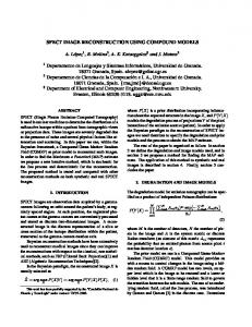
from a camera form a ruled surface called a cone-strip while the boundaries of cone strips are called intersection curves; these lie outside the actual surface in general. The conestrips are made up of multiple visual cone patches each of which has a rim segment, the part of the rim between successive frontier points. Figure 1 illustrates these definitions while [2, 5] provide details.
2. Theory X
1 0 0 1
1 0 0 1 0 1
Z 1 0 0 1
Y
11 00 11 00 00 11 11 00 11 00 00 11 11 00
Figure 1: 2-view visual hull: Rims are dashed curves; they intersect at frontier points; intersection curves are solid curves. Cone-strips and visual cone faces are also shown.
0 1 1 0 0 1
Frontier Point
Rim
2.1. Visual Hulls and the Rim Mesh
Figure 2: Top : 3-view case. Rims are dashed curves and intersecton curves are solid lines. X, Y and Z are frontier points. Below : The complete rim mesh. Every rim segment occupies a single visual cone patch.
The visual hull is the maximal shape that projects consistently into a set of silhouettes, and is obtained by intersecting visual cones from the corresponding calibrated viewpoints. Visual rays from a camera which grazes the true surface tangentially give rise to a smooth continous curve on the true surface called the rim [2, 16] or the contour generator and its projection in the image is the apparent contour. Rims from different cameras intersect on the surface at points called frontier points, which project to the respective apparent contours. The projected frontier points satisfy the 2-view epipolar tangency constraint [2] (these are the points of tangencies of tangents from the epipole to the silhouette which are also corresponding epipolar lines). The back-projection of points on the apparent contour produces viewing rays, each of which contributes a view edge to the visual hull polyhedron. At least one point on the view edge must touch the surface at a point on the rim. The view edges
The idea of epipolar nets [13] was refined into a formal representation called the rim mesh by [2]. The rim mesh is a combinatorial arrangement of rims on the surface (see Figure 2). Frontier points constitute its vertices and the rim segments between successive frontier points, form its edges. Each rim mesh edge thus corresponds to a visual cone patch. Patches on the surface bounded by different rim segments form faces in the rim mesh. The rim mesh itself contains only information about the arrangement of rims and their connectivity, not their geometric shape. The image based algorithm [2] computes the rim mesh only from silhouettes under some simplifying assumptions; it does not deal with occluded rims or objects with non-zero genus. An embedding of the rim mesh on the surface partitions it into patches where every patch is purely inside the visual hull but touches it along its boundary (along different rim seg2
v1
ments). This patch separates the object’s interior from a set of intersection curves, which lie outside the object in general. This property will be useful in our method.
v2
p1 p2
v4
p4
To Source
p3
(a)
To Sink
v3
2.2. The maximum flow problem
v1
Many global minimization and combinatorial optimization problems have been solved by formulating them as graphcut problems on network flows [20]. Given a flow network G(V, E) [20] with a source s and a sink t, a graph cut partitions V into S and T such that s � S and t � T . the maximum flow problem computes a flow with the maximum value. The max-flow min-cut theorem [20] shows that computing the maximum flow is equivalent to finding the mininum cost cut between s and t (the s-t min-cut). While s-t cuts can be computed efficiently, the more general multiway-cut problem (partitioning graphs into 3 or more subsets) is NP-Hard. In computer vision, [3, 8, 10] have used graph-cuts on geometric graphs while [11] has solved stereo, segmentation, multi-view reconstruction using energy minimization formulations via graph-cuts.
Even Level
p1 v2
p2 v3 v4 p3 p2
v2
v3 v1
v4
p4 p
Odd Level
3
p3
v3 v1 p1
p4
v4 To Source
To Sink
v2 (b)
3. Our Graph Cut Formulation
(c)
Figure 3: (a) 2D Visual Hull Polygon P = v1 , v2 , . . . , v4 from 2 views with p1 , p2 , . . . , p4 the apparent contours. (b) Embedding the 1D manifold in 3D (shown in bold). The vertical edges are shown (sparsely for clarity). (c) Two successive levels in the graph showing the connections to the source and the sink. (For clarity the grid is not drawn).
3.1. A 2D Overview Consider a 2D visual hull in flatland seen from two 1D cameras. Let P =v1 ,v2 ,. . . v4 be the visual hull polygon as shown in Figure 3(a). Different curves can give rise to P , however they must all touch every edge of P at least once. These contour points p1 ,p2 . . . p4 are the 2D apparent contours. If we knew their exact positions, we could partition the unknown curve into independent segments with fixed end-points. Without this information, we still know that, pi ∀i must lie somewhere on its respective edge (see Figure 3(a)). Now let us lift the 2D plane into a series of planes such that each individual segment bounded by two successive contour points lies in its own plane. See the illustration in Figure 3(b). The planes corresponding to every pair of adjacent curve segments are attached by vertical sheets such that the respective segments incident at a contour point on these different planes are connected through a vertical edge. We have taken a 1D closed manifold in 2D and embedded it in 3D by exploiting the silhouette constraints. Any curve that produces the visual hull P can be represented in this form. This representation allows us to map the true curve (or surface) to an s-t cut on a geometric graph. The graph construction for the 2D case is now described. Consider the 4-connected 2D grid graph GP (V, E) where V is the set of 2D voxels inside P and the points obtained by intersecting this grid with P . The set E contains all the edges connecting vertices in V on the underlying grid. While lifting P to multiple planes we make copies of GP and assign a copy GP i to each level i (imagine planes indexed by height). For every edge e of P , where segments i
and j are incident, a vertical sheet is created connecting GP i to GP j through surface vertices (representing surface points) on this edge e. Vertices for these surface points�are interconn nected by surface edges. Consider the graph i GP i along with all the vertical edges and surface vertices.In the even levels, the outside vertex vi is connected to the source while the boundary edges excluding the two edges incident on vi are connected to the sink. The source and sinks are reversed on the odd levels. The continuous curve will always map to a s-t cut (Figure 3(c)) if and only if the number of levels can be shown to be even. Visual hulls in 2D in the generic sense, always have an even number of edges, (since every camera contributes two half-planes and hence two distinct line-segments to the visual hull). This graph could grow quickly in size (especially in 3D) and could be considerably reduced when GP i in level i is limited to a potentially visibile region in the respective levels (see Section 3.4), assuming that the curve/surface cannot lie beyond the visibility boundary in this level. If it did, photo-consistency could never recover it anyway. 3
3.2. The 3D algorithm The 3D version is similar to the 2D case. The reconstruction surface is now a 2-manifold which must be lifted from 3D and embedded in a 4D geometric graph. P is the visual hull polyhedra and GP the associated 6-connected 3D grid graph consisting of voxels and surface points on P . The true surface touches faces of the visual hull mesh along rim segments (the edges of the rim mesh). Thus rims partition the actual surface into patches, each inside the visual hull but with boundaries, each forced to touch the visual hull along particular visual cone patches. Each level GP f is built from a rim mesh face f (This was also true in the 2D case, where the rim mesh was isomorphic to the 2D visual hull’s dual graph). In 2D, the subgraph GP i for level i was always connected to two subgraphs, each corresponding to vertex vi ’s neighbouring vertices in P . In 3D, the lateral connections for GP f are established based on which faces are adjacent to f in the rim mesh. Thus if f and g are adjacent faces in the rim mesh, P the sub-graphs GP f and Gg have lateral edges through the visual cone patch they share. Surface vertices on this cone patch are also interconnected by surface edges. The following result makes the max flow formulation possible in 3D.
Figure 5: An orthographic view of the subgraph for a single level. The graph show interior vertices, interior edges, surface vertices, surface edges and interior to surface edges. Rotated 3D views are shown in the inset circles.
Lemma 3.1 A surface map Mk , induced by the rim mesh from k views can be 2-colored.
3.3. Graph Construction (3D case)
Proof We prove this by induction: A rim divides the surface into 2 parts: front and back. Let us color them differently. Thus, M1 can be 2-colored. Assuming Mk can be 2-colored, we must prove that Mk+1 can also be 2-colored. After adding the (k + 1)th rim to Mk , swap colors of its front faces in the new map, Mk+1 , but leave the back faces untouched. This will always 2-color the newly created faces in Mk+1 , consistently with the old faces, unchanged from Mk . Thus Mk+1 can be 2-colored.
P P We first describe how to build sub-graphs GP f (Vf , Ef ) for each rim mesh face f . We then construct lateral edges and surface vertices to interconnect them. Vertices denote 3D points, sampled either inside the visual hull P on a regular grid M with unit resolution g or on the cone patches of P . V is(f ) denotes the visibility region for face f ; V is(f ) ⊆ M . The sets VfP and EfP are as follows :
VfP = {(x, y, z, f )} EfP
= {(u, v)}
u, v �
VfP
(x, y, z) � V is (f ) ×
VfP ,
(u, v) � M.
(1) (2)
GP f is sub-isomorphic to the grid graph of M . We denote the surface vertex set by Vps ; the set of surface edges by Eps and the set of surface to interior edges by Epi for patch p. Vps is defined as : Vps = {(x� , y � , z � )} where (x� , y � , z � ) is a surface point on cone patch p that cuts the grid lines of M . The set Epi is defined as : Epi = {(u, v)} u � VfP , v � Vps and f shares p with another rim mesh face. These edges join internal voxels to surface points along the grid lines. Eps is defined as: Eps = {(u, v)} u, v � Vps , and dist(u, v) � ≤ (3) ∗ g. These edges join proximal surface points on p. The interior vertices at the visibility boundary will connect to the Sink/Src vertices (Fig. 5). Let Tf be the set of those edges. Sf is the set of all edges connecting to the Src/Sink. Points on f ’s intersection curve form the vertex
Figure 4: 2-Coloring the Rim Mesh. (Left) Map induced by k-rims. (Right) Adding rim (k+1) 2-Coloring the rim mesh faces is equivalent to labeling the subgraphs GP i red and blue. For each red subgraph we set the source to be a subset of intersection curves belonging to this patch. The visibility computation (Section 3.4) finds a visibility boundary in this level which can be made the sink. For blue subgraphs, the sources and sinks are swapped. 4
set Rf . Vertices in Rf are connected to the closest interior grid vertices. Vertices in Rf are also connected to the Src/Sink by edges which make up the set Sf . Finally, we can now define G(V, E) as follows : V = E= (
�
�
( VfP ∪ Rf ) ∪ (
∀f
EfP
∀f
) ∪ (
�
�
Vps ) ∪ {s, t} (3)
∀p
(
Epi
∪ Eps ) ) ∪ Sf ∪ Tf
(4)
∀p
Interior vertices, interior edges, interior to surface edges have multiple copies in different subgraphs, if they are in the visibility regions for different rim mesh faces. Surfaces vertices and edges have single copies in G. The assignment of edge capacities in G is now described; c(u, v) is a measure proportional to the photo-consistency at the mid-point of vertices u and v. Due to different visibility computations, the 3D point corresponding to the edge (u, v) will have different photo-consistency measures in different visibility regions, each of which corresponds to a subgraph GP f . λ is a smoothness term explained in Sec. 3.5 and Cmax is a large constant. c(u, v) = 0.5 ∗ (C(u) + C(v)) + λ (u, v) � EfP c(u, v) = ∞ (u, v) � Sf or Tf c(u, v) = Cmax (u, v) � Epi
(5) (6) (7)
(u, v) � Eps
(8)
c(u, v) = λ
Figure 6: (a) Surface patch touching visual cone patches AB and AC at p1 and p2 . (b) The k ≥ 3 visibility region. (c) The same region with the Photo-Consistency costs.
insufficient views, the graph cut would lie along the visual hull cone patches at this face. With n views, the rim mesh has O(n2 ) faces. Without visibility regions, the vertex set V in the graph G(V, E) is O(n2 |G|) where |G| is the voxel count. Visibility shrinks V and makes it O(n|G|). This property makes our algorithm feasible for reconstruction in a fine volumetric grid. For a voxel v at level l, a vertex is present in the graph only if at least k cameras see it through the hole (set of visual cone patches) associated with this rim mesh face. A cone patch is shared between only two rim mesh faces. Since there are atmost n/k distinct groups of k camera sets, v can have atmost F ∗ |V |/k copies in different levels where F is the average number of cones patches in a rim mesh face ( � n, F = 3 in 2D).
An interior edge’s capacity c(u, v) reflects the consistency of the mid-point of voxels u and v. The surface edges have a constant capacity λ; increasing it reduces the overall curvature of the reconstructed rims on the surface. The high capacity on the surface to interior edges prevents the cutsurface from staying on the cone patch view edge if interior voxels are present. A higher value of Cmax would be suitable for smooth surfaces. When Vis(f) is empty, the cut is forced to go through these surface to interior edges resulting in a fully connected watertight cut-surface. Note that, the cut-surface could transition from one subgraph to another multiple times through the same cone patch. This would happen when the true surface is bitangent to the visual hull.
3.5. Energy Minimization Framework The color variance of a voxel projected into different views [12, 18], is used as a photo-consistency measure in energy functionals [10, 11, 8]. It is sensitive to outliers and improper sampling of voxels [15]. We need a robust measure as self-occlusions will produce outliers. We use a robust variance by picking the color variance of the most consistent rk ∗ k views within the k available views (rk is the inlier percentage). We assume lambertian surfaces, but a non-lambertian photo consistency [19] could also be incorporated. The minimum cut surface we recover is represented as an implicit surface S containing regular grid points (midpoint of cut edges) and surface points (constituting the reconstructed rims) that minimizes the following discrete en-
3.4. Computing Visibility For every rim mesh face, we find a region inside the visual hull, denoted by V is(f ), visible from at least k cameras. The apparent contours p1 and p2 on the visual cone patches AB and BC (see Fig. 6(a)) cannot be any further than A and C respectively. We treat the set of patches AB and BC as a hole in the visual hull, determine its at least k-visible region (Fig. 6(b)). Grazing views are avoided using a heuristic and robust cost based on photo-consistency (Fig. 6(c)) is computed at every vertex in Vis(f). If V is(f ) is empty due to 5
in the visual hull polyhedra, that project onto the apparent contour and lie between the end points of the image of the two cone-strip segments to be connected. We will call these the rim edges. The rim edges are important since they must belong to both the visual hull and the actual surface. Frontier elements can now be recovered by computing intersection between a pair of repaired cone-strips (circular list of rim edges and cone strip segments ordered on the apparent contour). Frontier elements are either (1) a view edge (2) a set of consecutive rim edges or (3) the end points of cone strips. Its image on the apparent contour could overlap with other frontier elements. A consistent ordering is enforced by using the epipolar tangency constraint in the images. While our graph-cut formulation can be generalized to complex closed 2-manifolds (its rim mesh is always 2colorable), the current rim mesh algorithm only works for genus-0 objects. While all viewpoints for convex surfaces are acceptable, for non-convex surfaces, only viewpoints where the rim is free of self-occlusion are allowed (corresponding apparent contour is free of T-junctions).
Figure 7: (a) Cone Strip Intersection for smooth silhouettes produce frontier points. (b,c,d) Frontier Elements are generalization of frontier points for discrete representations. (e) Cone Strips under perfect conditions. (f) Broken cone-strip segments. (g) Repaired Cone-strip. ergy functional E(S). E(S) =
�
C(v) + λ
(9)
4. Experimental Results
v�S
where v denotes a point in S, C(v) is its photo-consistency whereas λ is a smoothness parameter weighting the smoothness against the photo-consistency. Our smoothness term is spatially constant and corresponds to minimizing the Manhattan area (equivalent of Manhattan distance in 2D) of the cut-surface. The total smoothness cost is λ ∗ |CS | where CS is the set of cut edges. Our maximum flow algorithm computes the global minimum of this energy function E(S). In our formulation, the energy functional does not have any silhouette terms.
We solve max-flow using an algorithm shown to work efficiently on grid graphs [11]. The visibility regions are computed using segment-triangle intersection tests but this could be accelerated by multi-resolution methods and graphics hardware based volume rasterization. We demonstrate results on synthetic sequences (512 × 512 images): Pear and Sphere and a real data (502 × 760 images): Head. Pear Sequence: Rows 1 and 2 of Figure 8: Figure 8(a,c) shows the visual hull computed from 4 views and the corresponding rim mesh containing 10 frontier points is shown in Figure 8(e). 12 color images were used with minimum visibility k set to 5 views. The reconstruction was done on a 100 × 130 × 130 grid; the resulting graph had 0.4 million vertices and 1.1 million edges and the reconstructed surface had 43K points. The reconstruction took about 6 minutes but max-flow used only 10 − 12 seconds. Most of the time was spent in computing the photo-consistency costs in different visibility regions and the graph cut itself is much faster. Figure 8(b,d) shows the 2-coloring of the reconstructed surface separated from each other by the reconstructed rims (in white). Figure 8(f) shows the reconstructed surface with texture while Figure 8(g,h) show the ground truth and reconstructed mesh model respectively. Sphere Sequence: Row 3 of Figure 8: The visual hull was built from 6 silhouettes while 12 color images were used with k = 4 for computing photo-consistency. A 100 × 100 × 100 grid produced a graph with 0.44 million vertices and 1.3 million edges and a reconstructed surface with 40K points. Two different reconstructions are shown in Figure 8(b,c) with a higher value of λ in (b) followed by
3.6. Robust Computation of Rim Mesh Lazebnik’s rim mesh algorithm [2] assumes smooth silhouettes and perfect data (good segmentation, calibration). Discretization or calibration noise makes the rim mesh unstable, as it causes missing frontier points, due to the problem of lost tangency [5] or perturbs their consistent ordering. We relax the need for perfect data by robustly computing a consistent rim mesh where frontier points (Figure 7(a) are replaced by generalised frontier elements which could be edges or facets as shown in Figure 7(b,c,d) for 2-views) or a contiguous sequence of edges for 3 or more views. Exact polyhedral visual hulls (EPVH) as computed by [5] contain all the facets constituting the broken rim segments as shown in Figure 7(f). These segments can be recovered from EPVH by checking its facets for co-planarity with the camera center and then sorting them on the apparent contour. These cone-strip segments are then ordered along the apparent contour. The broken cone-strips can be repaired (see Figure 7(g)) by finding the unique sequence of edges 6
a lower value in (c). The rim curves have a higher curvature for a lower value of smoothness cost λ. The reconstructed triangulated sphere model is shown in Figure 8(d). Head Sequence: Rows 4 and 5 of Figure 8: This is a turntable sequence with 36 images; Figure 8(a) shows four of them. 8 images were used to build the visual hull (see Figure 8(b). The rim mesh (see Figure 8(c)) has 56 frontier elements and 58 faces. Many faces are clustered at the top and bottom of the head model and contribute very small or degenerate patches to the final model. k set to 10 views with the inlier fraction, rk = 0.8 in order to deal with self-occlusions while computing photo-consistency. A 120 × 160 × 170 grid produced a graph with 1.47 million vertices and 4.5 million edges and a reconstructed surface with 108K points. Running time was 75 minutes with maxflow using only about 30 − 50 seconds. The reconstructed model recovers surface detail and is rendered from different views alongwith texture in Figure 8(d-h).
[4] J. Isidoro and S. Sclaroff, “Stochastic Refinement of the Visual Hull to satisfy photometric and silhouette consistency constraints,” In Proc. ICCV, pp. 1335-1342, 2003. [5] J.S. Franco and E. Boyer, “Exact Polyhedral Visual Hulls,” In BMVC’03, Vol. I, pp. 329-338, September 2003. [6] O. Faugeras and R. Keriven, “Complete Dense Stereovision Using Level Set Methods”, In Proc. ECCV98, pp. 379-393. [7] C.H. Esteban and F. Schmitt, “Silhouette and Stereo Fusion for 3D Object Modeling,” CVIU, Special Issue on Modelbased and image-based 3D Scene Representation for Interactive Visualization, 96,3,367-392, Dec 2004. [8] S. Paris, F. Sillion and L. Quan, “A Surface Reconstruction Method Using Global Graph Cut Optimization,” In Proc. of Asian Conference on Computer Vision, January 2004. [9] D. Snow, P. Viola and R. Zabih, “Exact Voxel Occupancy with Graph Cuts”, In Proc CVPR, 2000. [10] S. Roy and I. Cox, “A maximum-flow formulation of the ncamera stereo correspondence problem,” In Proc of 6th Internation Conference on Computer Vision pp. 492-502, 1998.
5. Conclusions and Future Work We presented a multi-view surface reconstruction approach which uses color-consistency and silhouettes to reconstruct a closed surface while exactly satisfying silhouette constraints and minimizing an energy function based on photoconsistency and smoothness. We transformed the reconstruction problem into solving max-flow / min-cut on a geometric graph derived from the rim mesh of the object. This framework which enforces silhouette constraints exactly and excludes it from the energy minimization is the main contribution of this paper. We have demonstrated our approach on real and synthetic data. Future work will consist of improving the efficiency and robustness of the photoconsistency measure as well as developing better shape priors. Work is also needed on robust computation of the rim mesh for more complex surfaces so that our work can be extended to objects with arbitrary topology. Acknowledgements We thank J.S. Franco and E. Boyer for the EPVH library [5] and Y. Boykov and V. Kolmogorov for the max-flow software [11]. The support of Siemens Corporate Research, Princeton, USA and the NSF Career award IIS 0237533 is gratefully acknowledged.
[11] Y. Boykov and V. Kolmogorov, “An Experimental Comparison of Min-Cut/Max-Flow Algorithms for Energy Minimization in Computer Vision,” PAMI, 26,9,1124-1137, Sep 2004. [12] K.N. Kutulakos and S.M.Seitz, “A Theory of Shape by Space Carving,” In Proc. of ICCV, pp. 307-314, 1999. [13] G. Cross and A. Zisserman, “Surface Reconstruction from Multiple Views Using Apparent Contours and Surface Texture”,In NATO Advanced Research Workshop on Confluence of Computer Vision and Computer Graphics 2000, pp. 25-47. [14] S. Sullivan and J. Ponce, “Automatic Model Construction, Pose Estimation, and Object Recognition from Photographs using Triangular Splines,” PAMI, 20,10,1091-1096,1998, [15] G. Slabaugh, B.W. Culbertson, T. Malzbender, M.R. Stevens and R. Schafer, “Methods for Volumetric Reconstruction of Visual Scenes,” In IJCV, Vol. 57(3), pp.179-199,2004. [16] R. Cipolla and P. Giblin, “Visual Motion of curves and surfaces,” Cambridge Univ. Press, 2000. [17] D. Scharstein and R. Szeliski, “A Taxonomy and Evaluation of Dense Two-Frame Stereo Correspondence Algorithms,” In Int. Journal of Computer Vision, Vol 47(1-3) pp 7-42,2002.
References
[18] S.M. Seitz and C.R. Dyer, “Photorealistic Scene Reconstruction by Voxel Coloring,” In Proc CVPR, pp.1067-1073, 1997.
[1] A. Laurentini, “The Visual Hull Concept for Silhouette-Based Image Understanding”, PAMI 16,2(Feb 94),150-162.
[19] R. Yang, M. Pollefeys and G. Welch, “Dealing with Textureless Regions and Specular Highlights: A Progressive Space Carving Scheme Using A Novel Photo-consistency Measure,” In Proc ICCV , pp. 576-585,2003.
[2] S. Lazebnik, E. Boyer, and J. Ponce, “On Computing Exact Visual Hulls of Solids Bounded by Smooth Surfaces,” In Proc. CVPR, pp. 156-161, 2001.
[20] T.H. Cormen,C.E. Leiserson,R.L. Rivest and C. Stein, “Introduction to Algorithms”, MIT Press, 2nd. Ed., 2001.
[3] G. Vogiatzis, P.H.S. Torr and R. Cipolla, “Multi-view stereo via Volumetric Graph-cuts”, In Proc. CVPR, 2005.
7
Figure 8: (Rows 1,2) Pear: 12 images: (a) Visual hull (b) 2-colored reconstructed surface (rim curves are white). (c & d) Visual Hull and the reconstructed surface in another view. (e) The rim mesh (10 frontier element, 12 faces). (f) The reconstructed surface with texture. (g,h) Ground truth and reconstructed mesh respectively.(Row 3) Sphere: 12 images: (a) Visual hull (b) Reconstruction with higher smoothness cost; (c) with lower smoothness cost. (The rims curves on the surface have different curvature) (d) Reconstructed mesh. (Rows 4,5) Head: 36 images: (a) 4 of them shown (b) Visual hull from 8 silhouettes (c) Rim mesh (56 frontier elements, 58 faces). (d) Reconstructed point cloud (e-h) shown with texture.
8