Multi-View Video Packet Scheduling

Multi-View Video Packet Scheduling Laura Toni, Member, IEEE, Thomas Maugey, Member, IEEE, and Pascal Frossard, Senior Member, IEEE

arXiv:1212.4455v2 [cs.MM] 28 May 2013

Abstract In multiview applications, multiple cameras acquire the same scene from different viewpoints and generally produce correlated video streams. This results in large amounts of highly redundant data. In order to save resources, it is critical to handle properly this correlation during encoding and transmission of the multiview data. In this work, we propose a correlation-aware packet scheduling algorithm for multi-camera networks, where information from all cameras are transmitted over a bottleneck channel to clients that reconstruct the multiview images. The scheduling algorithm relies on a new rate-distortion model that captures the importance of each view in the scene reconstruction. We propose a problem formulation for the optimization of the packet scheduling policies, which adapt to variations in the scene content. Then, we design a low complexity scheduling algorithm based on a trellis search that selects the subset of candidate packets to be transmitted towards effective multiview reconstruction at clients. Extensive simulation results confirm the gain of our scheduling algorithm when inter-source correlation information is used in the scheduler, compared to scheduling policies with no information about the correlation or non-adaptive scheduling policies. We finally show that increasing the optimization horizon in the packet scheduling algorithm improves the transmission performance, especially in scenarios where the level of correlation rapidly varies with time. Index Terms Foresighted packet scheduling, source correlation analysis, multiview streaming, interview correlation, rate-distortion optimization, multimedia communication.

I. I NTRODUCTION Advances in interactive services and 3D television have paved the road to multiview video applications, in which multiple sources acquire and transmit several correlated media streams [1]–[4]. Multimedia wireless sensor networks and multi-camera video systems are typical examples of multiview setups. The flexibility and the interactivity offered by such applications however come at the price of increased storage/bandwidth requirements. To overcome these limitations, the coding and transmission schemes need to properly exploit the correlation among sources, in order to provide effective image quality in resources constrained environments. In this context, we aim at providing insights on how resource allocation strategies can benefit from correlation information in a multi-camera scenario, in which neighboring cameras acquire the same scene but from different perspectives. This scenario results in spatial correlation between the information streams, since cameras typically have overlapping fields of view, in addition to temporal correlation between frames acquired consecutively by the same camera. This spatial-temporal correlation can be exploited either at the source (e.g., by joint encoding of the different sources) or at the decoder side (e.g., by joint reconstruction of the different images). In this work, we consider the latter case and we show how the packet transmission scheme can be opportunistically adapted to satisfy network constraints, when the source correlation is exploited at the decoder for image reconstruction. In more details, the proposed framework targets the optimization of resource allocation schemes for the transmission of correlated sources under delay and bandwidth constraints. Rather than focusing here on source coding aspects, we are interested in a scenario where each camera independently acquires part of a scene with no communication between cameras. The encoded views need to be gathered by a gateway or a wireless access point (AP) (see Fig. 1), which then forwards packets to clients interested in decoding (part of) the 3D scene. Assuming that network resources are constrained, only a subset of the camera images can be transmitted to the clients. The encoded views are transmitted with a correlation-aware packet scheduling algorithm driven by the gateway or the AP. This centrally coordinated scenario is quite typical in practice, and in particular in IEEE 802.11 wireless networks. In these networks, the Point Coordination Function (PCF) is one of the common solutions supported by Medium Access Control (MAC) layer to organize data transmission [5], [6]. At higher layers, master routers or home gateway devices are also used as central controllers for network services and devices [7], [8]. The packet scheduling algorithm filters packets to reduce the transmission cost and satisfy the resource constraints in the system under the assumption that the images are jointly reconstructed at decoder. In order to optimize the reconstruction quality, one has however to properly select the packets to be transmitted, along with their transmission schedule. For example, the frames that are highly correlated to packets already available at the decoder can have a low priority in the scheduling algorithm. This is due to the fact that they can be reconstructed from the correlated frames at the decoder side even if they are actually not transmitted. On the other hand, frames that have only a low correlation with previously transmitted data should be prioritized in the scheduling since they would be reconstructed at a poor quality if they are not transmitted. ´ L. Toni, T. Maugey and P. Frossard are with Ecole Polytechnique F´ed´erale de Lausanne (EPFL), Signal Processing Laboratory - LTS4, CH-1015 Lausanne, Switzerland. Email: {laura.toni, thomas.maugey, pascal.frossard}@epfl.ch.

2

Figure 1.

Multi-camera system, with bandwidth bottleneck at the access point.

We propose a novel rate distortion (RD) model that estimates the distortion in scene reconstruction from multiple correlated images. Based on this model, we build a scheduling technique that minimizes the distortion in the scene reconstruction and adapts the transmission scheme to temporal variations of the scene content and correlation level. The proposed scheduling algorithm optimizes the long-term utility function with refinement at each transmission opportunity. For such an algorithm to reach optimality though, a large time horizon has to be considered in the optimization, which leads to high computational complexity. Thus, we propose a suboptimal trellis-based algorithm that is able to reduce the complexity while still preserving most of the benefits of correlation-aware scheduling optimization. Simulation results demonstrate that the proposed scheduling algorithm outperforms correlation-agnostic scheduling policies or static camera selection algorithms. This shows the need of correlation-aware scheduling policies in multiviews systems, which are able to efficiently share network resources among cameras, while rate allocation (RA) techniques proposed in the literature cannot solve such a scheduling problem, since they usually do not consider correlation between sources [9], [10]. The remainder of this paper is organized as follows. Related works on multiview data gathering are described in Section II. In Section III, some technical preliminaries are given and our new RD model is introduced. The packet scheduling problem is formulated in Section IV and the trellis-based optimization solution is provided in Section V. In Section VI, we discuss the simulation results, and we conclude in Section VII. II. R ELATED W ORKS In this section, we first provide a general overview of the most relevant works from the literature that focus on multi-camera streaming and we highlight the key differences with our work. Then, we describe in more detail the research work in resource allocation and correlation-aware multiview streaming. In multiview systems, prior studies usually addressed two main open problems: i) how to efficiently encode distributed sources, ii) how to efficiently deliver information to users in different applications. To answer the first question, distributed source coding (DSC) has gained attention as new coding paradigm [11], [12] to exploit source correlation. When no communication is assumed between cameras during the coding process, DSC allows the encoding to stay simple by shifting the computational complexity to the decoder. Research on DSC, as well on distributed video coding (DVC), has been mainly focused on optimizing the coding scheme, given an a priori knowledge on the correlation, i.e., given an a priori side information (SI) [13]–[15]. Thus, the selection of sources that can be used for the generation of SI is usually assumed to be known; the optimization of this selection is still an open problem. Even if many works have studied DSC in multiview applications, an optimization framework that is able to exploit in the most efficient way the source correlation level is still missing. In our paper, similarly to the DSC framework, we consider that the cameras do not communicate with each other but rather exploit the source correlation in the packet scheduling process. Even if this is not considered in this paper, our framework also applies to cameras streams encoded by DSC. It represents a complementary solution to DSC in the design of distributed camera systems. In the second set of works that optimize the delivery of multiview data, some prior studies address the problem of providing interactivity in selecting views, while saving on transmitted bandwidth and view-switching delay [2], [16]–[20]. The work in [2] is mainly focused on coding views with a minimum level of redundancy in order to simplify the view switching, and the works in [18], [21] optimize the selection of views to be encoded and transmitted based on the user interest. The authors in [19], [22] investigate the transmission of multiview video coded streams on P2P networks and IP multicast, respectively. These works mainly focus on the coding aspects and DSC is often proposed as a solution to reduce encoding complexity [23] or to provide interactive access to the different views [24]. The work proposed in this paper is rather defined as a rate allocation problem in multi-camera systems. Multi-camera resource allocation solutions in the literature often ignore the dynamic correlation between sources and rather focus on optimizing the resources for each camera independently. In other words, they usually optimize the scheduling policy in evaluating the cost, the distortion gain and the time constraints of each camera separately and ignores the possible correlation among cameras. This may result in suboptimal allocation of the network resources. Resource allocation techniques have for example been considered in [10] for video surveillance systems, in which each of the camera captures and transmits the video information in a multihop

3

network. The optimization of the resource allocation (i.e., the time sharing between sources) is based on both the network and source information, but ignores the correlation between the sources. In a more general resource allocation framework, few works have introduced the sources correlation in the optimization of transmission schemes. A multi-party 3D tele-immersive system is considered in [25], where correlated views are rendered together to create a common virtual environment among all participants. These participants are distributed over an overlay network and can gather information from neighboring nodes. Source correlation is taken into account to dynamically optimize the multicast topology for content delivery between nodes involved into the multi-party 3D tele-immersive session. In [26], a three-step approach is proposed to optimize the resource allocation between spatially correlated sources for multi-cell frequency-division multiple access (FDMA) networks. However, multimedia transmission is not considered in the optimization. In [27], the level of spatial correlation between sources has been considered at the MAC layer for wireless sensor networks. The authors assume that the network needs to estimate an event S. Due to the correlation between neighboring sensors, only part of them might be selected for sending information to the sink, so that the transmission data rate is limited. The MAC protocol prioritizes the access to representative nodes, i.e., nodes with reduced levels of correlation. The same intuition has been considered in [28] and applied to multimedia streaming. A spatial correlation model for visual information in wireless multimedia sensor networks (WMSNs) has been proposed, introducing an entropy-based analytical framework to evaluate the visual information offered by multiple cameras. When the network resources are insufficient the cameras that maximize the joint entropy in a camera set are selected for transmission. The model however only solves a static correlation-based camera selection technique, while we consider a dynamic correlation-based packet scheduling optimization in our work. In particular, the framework in [28] can be seen as a particular case of our problem, where both cameras and scene content are static. The correlation model proposed in [28] has been also used in [29], where the problem of efficient gathering of visually correlated images from multiple sensors has been investigated. The scheduling optimization is aimed at reducing the energy consumption during transmissions by exploiting a correlation-aware differential encoding technique. However, the model is highly sensitive to transmission failures. Moreover, the cameras grouping optimization is based on the assumption of a static correlation, which does not hold in dynamic scenarios. Our work is substantially different from [29], since we propose a packet scheduling optimization that i) is able to adapt to correlation variations in dynamic scenes, ii) considers independent source coding (i.e., it preserves simplicity at the source side). Finally, it is worth noting that the correlation between cameras might be exploited not only for DSC or resource allocation techniques, but also for error resilience. For example, the correlation between views is implicitly considered in [30]. The authors propose an optimized interactive multiview streaming over wireless wide area networks (WWAN), where a cooperative peer-to-peer repair technique is considered to alleviate packet losses. There are important differences between the above works and the study proposed in this paper. First, we focus our attention on the important problem of optimizing scheduling algorithms such that view correlation can be exploited efficiently at the decoder. Second, even if some other works have investigated resource allocation techniques for multiview scenarios, dynamic view correlation and dynamic packet scheduling solutions are not studied in the literature related to multi-camera systems. This is exactly what we propose to address in this paper. III. F RAMEWORK We now describe the framework considered in our work. First, we present the multi-camera system and describe the multiview acquisition and transmission processes. Then, we introduce the scene reconstruction method and show that the correlation between cameras plays a crucial role in the reconstruction of missing frames at the decoder. Finally, we propose a new rate-distortion model for the representation of the 3D scene information. A. Multi-camera system We consider M cameras that acquire images and depth information of a 3D scene from different viewpoints. The images acquired by the M correlated cameras need to be collected by a common AP that eventually transmits (part of) the 3D scene information to clients, which are all interested in receiving all video streams. Due to bandwidth constraints in the communication system (e.g., on the wireless channel, or on the path between AP and clients), it might not be possible to transmit all the frames from all the cameras to the clients. Thus, at each transmission opportunity, it is important to accurately select which images have to be scheduled and which ones can be sacrificed (i.e., not transmitted), such that the average distortion is minimized. However, depending on the camera arrangement and the scene information, the frames acquired from the different cameras might be correlated in both time and space. First, each camera acquires temporally consecutive frames, which are correlated, especially for static or low-motion 3D scenes: this is the temporal correlation in image sequences. Then, neighbouring cameras might acquire overlapping portions of the same scene; this leads to correlated frames due to the spatial correlation between multiview cameras. Both the temporal and the spatial correlations might help in reconstructing the overall scene information if some images are missing at the decoder. We address the frame selection problem as a resource allocation problem that takes into account the level of correlation among cameras in a novel packet scheduling algorithm. We assume a model in which there is no communication among cameras in

4

order to save bandwidth and power. The only minimal information that is known a priori is the position of the cameras, which is possibly updated when cameras change positions in dynamic settings. Along with depth information, each camera is able to estimate its influence on its neighbors and in particular the contribution that it can offer in the reconstruction of neighbor views. We propose below a novel correlation model where each camera can predict the correlation level with neighboring cameras, without global depth information. This local correlation level, which is a set of simple values representing the influence of the camera in the reconstruction of the neighboring ones, is sent by each camera to the scheduling engine. Then, we consider that each encoded image at a given time instant from a particular camera is packetized into a data unit (DU) and stored in the camera buffer. Each data unit contains texture and depth information about the 3D scene. All the camera DUs are possible candidates for scheduling. We further assume that the transmission is based on a Time Division Multiple Access (TDMA) model where no more than one DU might be scheduled in any TDMA slot. Once a DU is scheduled for transmission, the channel stays busy for one or multiple time slots, until the current DU has been completely transmitted.1 Due to streaming delay constraints, the DU needs to be received before a playback deadline, denoted by TD , in order to be useful for decoding. This means that a DU acquired at the time t stays useful till time t + TD . Data units that have no chance to be received on time are not considered for scheduling and simply dropped by the cameras. We also assume that the communication channel is lossless such that all the transmitted DUs are correctly received by the access point and subsequently the clients. It follows that packets that are not available at decoder have been skipped by the scheduler, and not lost due to unreliable communication. In this framework, our goal is to propose a correlation-aware scheduling algorithm that selects DUs from different cameras in such a way that the overall distortion in the reconstruction of all camera views is minimized under the bandwidth constraints. B. Scene Reconstruction We describe now the scene reconstruction process, which will help to better understand the benefits of exploiting the spatial and temporal correlation of the images. At the receiver side, each frame is decoded independently. The images that have not been transmitted are estimated based on time and/or view interpolation algorithms using information from neighboring frames. More precisely, for the interpolation of a missing view n, the receiver uses images from neighboring cameras with help of depth image based rendering (DIBR) techniques (Fig. 2(a)). Typically, DIBR algorithms use depth information in order to estimate by projection the position of pixels from view k in the missing view n. The projected pixels are generally of good precision (depending on the accuracy of the depth map [31]) but do not cover the whole estimated image, due to visual occlusions. As shown in Fig. 2(b), one can build a binary mask that describes the occluded regions. Then, by merging the estimations obtained by the projections of different neighboring views, we obtain different reconstructed regions in the interpolated image. This can be summarized in a global occlusion map with different regions corresponding to the different occlusions. In the example in Fig. 2(b), the reconstructed scene is subdivided into three regions, each of them is characterized by the set of neighboring views that contribute to the scene reconstruction. In particular, the blue region (which represents 7% of the total scene) is reconstructed based on the estimation from only the view n + 1, while for the yellow one (which represents 9% of the total scene) the estimation from view n − 1 is considered. The remaining 84% of the scene (i.e., the green region) is reconstructed by merging estimations from both views. The principle for temporal extrapolation is the same. The decoder uses the available past frames to reconstruct a missing frame. The past frames cannot be used to estimate the whole missing image because of occlusions and object motion. The regions where the past frames could give some useful information are computed similarly to the occlusion map in the view interpolation case. The global map with the different prediction regions is used to decide on the best interpolation method for the missing frames at the decoder. An example of multiview video reconstruction is depicted in Fig. 3, for the case of 8 cameras that acquire several temporally consecutive frames. The goal of the decoder is to reconstruct all the frames in time and space, even if only part of them have been received (dark colored boxes in Fig. 3). In this example, we consider that each frame is correlated with frames of the two neighboring views in space, and with the two temporally successive frames (of the same view). If one or more of these correlated frames are missing, the received frames can contribute to the estimation of the missing data (light colored boxes in Fig. 3). In order to avoid error propagation, we consider that only the received frames can be used to reconstruct the missing ones (i.e., reconstructed frames are never used for estimation of other missing frames). Note that we consider temporal estimation only in the forward direction for the sake of simplicity. Our model can however be extended easily to include temporal interpolation in the backward direction too (i.e., from future frames). Finally, a missing frame cannot be reconstructed (white boxes in Fig. 3) when all its correlated frames are missing too. C. Rate-Distortion Model We now propose a novel rate-distortion model adapted to the scene reconstruction framework described above. The m-th camera at time t, acquires the image Ft,m and compresses it at a rate of Rt,m bits per pixel (m = 1, . . . , M ). A subset of the compressed images captured by all cameras is transmitted to the decoder, which targets the reconstruction of the full scene. If 1 From

here onwards, we assume the time axis discretized in slots (or scheduling slots) of length equal to the TDMA slot duration.

5

3D scene

vie

w

Camera n-1

1

n-1

w

n+

vie

DIBR

DIBR

Camera n+1

Two estimations

Camera n

(a)

1 93%

estimation from view n-1

0 7%

11 84%

1

10 9%

01 7%

91%

estimation from view n+1

09%

Two estimations

Mask for each estimation

Global occlusion mask

(b) Figure 2. Example of DIBR image estimation at decoder. (a) the central view n is estimated from the two neighboring views n − 1 and n + 1. (b) the occlusion maps corresponding to the two estimations are merged in order to obtain a global occlusion map with 3 regions. The percentage numbers in the masks indicate the portion of the frame dedicated to each region.

the frame Ft,m is available at the decoder, the distortion is directly dependent on the compression or the source rate. If Ft,m is missing at decoder, it is reconstructed from the available neighboring frames (in time and space), as described in the previous section. The overall distortion of the scene at instant t is thus expressed as Rt ) = Dt (R

M X 1 Rt ) Dt,m (R w m=1 m

(1)

where wm represents the relative importance of a given camera view. It permits to give a different weight to each camera view in the distortion evaluation (e.g., the central camera might be preferred to the lateral ones) and it reflects the relative interest that clients have in each camera stream. In our problem formulation, the weight parameter is assumed to be given as a priori information. The rate vector R t , defined as R t = [Rt,1 Rt,2 . . . Rt,M Rt−1,1 . . . Rt−1,M . . . Rt−ρT ,1 . . . Rt−ρT ,M ]T , represents the size (in bpp) of the frames received from the different cameras (m = 1, . . . , M ) in a window of time of size ρT , which can be used for the reconstruction of Ft,m . The parameter ρT defines the maximum number of frames that can R t ) is the distortion of the m-th view at instant be considered in temporal interpolation at the decoder. The distortion Dt,m (R t. For each view m acquired at the instant t, we further decompose the frame into regions sj and we denote by St,m the set of such regions. For each sj ∈ St,m , we denote by α(sj ) the relative area of the frame dedicated to the region sj , such

6

Figure 3. Example of frames reconstruction in multiview video setup, where each frame is correlated with the frames of two neighboring views and with the two temporally consecutive frames (of the same view). Missing frames are reconstructed from information in the correlated frames that are available at decoder. Received frames are represented in the figure by dark colored boxes, the reconstructed ones by light colored boxes. White boxes represent frames that cannot be reconstructed from the received frames.

P that sj ∈St,m α(sj ) = 1. In Fig. 2, for example, the frame acquired from the central camera is subdivided in three different regions: the blue, the yellow, and the green ones, with α(sj ) corresponding to 0.07, 0.09, and 0.84 respectively. Then, a mapping function φ j,m,t describes which of the neighboring frames can contribute to the reconstruction of the region sj of the m-th view at time t. In the absence of temporal correlation, the spatially neighboring views only are considered for frame reconstruction. This means that φ j,m,t = [φj,m,t (1) . . . φj,m,t (M )], where φj,m,t (k) = 1 if the k-th camera is correlated with the region sj of the frame Ft,m and φj,m,t (k) = 0 otherwise. In this case, R t reduces to R t = [Rt,1 Rt,2 . . . Rt,M ]. When both spatial and temporal correlations are used in the reconstruction, the matrix φ j,m,t becomes φ j,m,t = [φj,m,t (1) . . . φj,m,t (M ) φj,m,t−1 (1) . . . φj,m,t−1 (M ) . . . φj,m,t−ρT (1) . . . φj,m,t−ρT (M )] where ρT is the number of past frames that can be considered for the reconstruction of the current image. Equipped with the R t ) becomes the sum of the distortion in each part stj of the frame at instant t: above notation, the distortion Dt,m (R  P φ j,m,t · R t ] if the view is not received sj ∈St,m α(sj )d [φ Rt ) = (2) Dt,m (R d [Rt,m ] otherwise. Finally, the distortion functions d[R] in Eq. (2) can be evaluated from the general expression of the RD function of an intra-coded frame with high-rate assumption [32]: d[RI ] = µI σI2 2−2RI

(3)

where RI is the number of bits per pixels and is equal to the sum of the rates that contribute to the current region, σI2 is the spatial variance of the frame and µI is a constant depending on the source distribution. It is worth noting that the model of Eq. (3) has been chosen because it is quite simple and yet accurate. However, our packet scheduling framework is general and other source rate-distortion functions could be used in Eq. (2). IV. PACKET S CHEDULING A LGORITHM We discuss in this section a novel packet scheduling framework for wireless multiview camera system that uses the ratedistortion model proposed in the previous section. Then, we propose a novel problem formulation for rate-distortion optimal packet scheduling. A. Transmission policy We consider a channel with successive time slots for packet transmission. Each time slot represents a transmission opportunity. The objective is to select which DU should be transmitted at each available time slot, in order to maximize the quality at the decoder under the playback delay constraint given by TD . A greedy hence myopic strategy can choose the scheduling policy by selecting to transmit at each time slot the frame that minimizes the overall distortion at decoder. However, such a scheduling solution does not necessarily optimize the overall distortion since it does not consider a long term optimization objective. A less myopic scheduling leads the scheduler to allocate more fairly all the views of the camera set with a more global distortion objective. Thus, in the following we optimize the packet scheduling strategy over a finite time horizon that is generally larger than one transmission time slot.

7

The delay TD as well as any temporal parameter introduced in the following is expressed in terms of time slots for the sake of clarity. We denote by t the time slot at which we optimize the scheduling policy for a time horizon of K time slots. We consider an online optimization with no a priori information about the video sequence. However, we allow a latency of K slots between the acquisition and the scheduling process, in such a way that, at time t, the characteristics of frames acquired up to the time slot (t + K − 1) are available to the scheduler. In more details, at the time instant t, all the frames from all the views acquired in the interval [t − TD + 1, t + K − 1] are possible candidates for transmission except those that have been scheduled already. They form a set of cardinality L. Let the l-th DU be characterized by its size Bl in bits2 , its acquisition time slot TA,l (i.e., the instant at which the frame is acquired), its expiration deadline TTS,l = TA,l + TD , and its transmission policy πl : {al (1) . . . al (K)} in the next K time slots. A transmission policy πl at time t is a binary vector according to which the DU l is allocated for transmission over the time horizon [t, t + K − 1]. Let A = {0, 1} be the action space and al (k) ∈ A the scheduling action taken for the DU l at the k-th slot of the optimization. In particular, al (k) = 1 means that the data unit l has to be sent at time (t + k − 1). As the channel is lossless, we assume that each DU is scheduled at most once during its lifetime and that each transmitted DU is sent entirely. In order to avoid transmitted DUs whose deadline has expired, we impose that at the k-th slot (with k = 1, . . . , K) only DUs acquired in the time interval [t − TD + k + 1, t + K − 1] are candidates for being transmitted at time (t + k). Finally, we denote by π = [π1 . . . πL ]T the scheduling policy for the L candidate DUs at time t. Each policy π leads to a particular distortion on the client side. In this work, we seek the best policy π ⋆ that is able to minimize the expected distortion while satisfying the channel constraints. The scheduling policy is refined at next transmission opportunity based on the newly acquired frames. This means that a scheduling policy can change over time. In particular, among the best set of DUs selected for transmission, the DU scheduled in the first time slot is sent, while the scheduling is not guaranteed for the other DUs. For example, a DU planned for transmission by the scheduling policy computed at time t might actually never be transmitted if a future frame with higher importance takes its transmission slot. In this way, the refinement of the scheduling policy compensates for the limited knowledge of the video sequence that is imposed by the online nature of the algorithm. We formally define below the packet scheduling problem in our new framework. B. Problem Formulation We first consider the scheduling problem for a single DU. In this case, the transmission rate is denoted by "K # X R (πl ) = Bl al (k) k=1

PK

where k=1 al (k) is equal to 1 is the DU l is scheduled for transmission in the k-th slot, and equal to 0 otherwise. The overall distortion is evaluated as  PK Dl (Ψ {H}) if k=1 al (k) = 0 D (πl , H) = (4) Dl (Ψ {H ∪ l}) otherwise where H is the set of the DUs already transmitted in the time slots before t (i.e., H represents the scheduling history), and Dl is the overall distortion level derived from Eq. (2), where the subscripts {t, m} have been replaced by the subscript l to describe the data unit l. The function Ψ {H} evaluates the received rate vector R of the M views acquired in the last ρT instants given the set of transmitted DUs H. In particular, each element j of the vector R is set to Bj if the j ∈ H, and to 0 otherwise. The evaluation of Dl obviously involves the size and the prediction maps of the data unit, namely Bl and {φj,l }. For the sake of clarity, we omit this dependency in our equations. We now consider the rate and distortion for multiple DUs. In the joint scheduling of multiple DUs, we evaluate the average distortion and rate for a set of scheduling policies π = [π1 . . . πL ]T . This outlines the dependency between DUs in the packet scheduling optimization. The average rate for a set of L DUs with a transmission policy π is thus given by "K # X X X π) = R(π R (πl ) = Bl al (k) . (5) l

l

k=1

The derivation of the average distortion is not as straightforward as the one of the average rate. In particular, the rate of a given DU only depends on the scheduling policy for that DU, while the distortion for a given DU depends on the scheduling policy of the correlated DUs π , H) = D (π

L X 1 Dl (Ψ {H ∪ Pπ }) wl l=1

2 The

size of a DU includes the size of both texture and depth data.

(6)

8

where Dl is the distortion for the reconstructed DU l, given the scheduling policy π , and Pπ is the set of DUs scheduled in the time slots [t, t + K − 1] based on the scheduling policy π . Note that, among the DUs in Pπ , the frames correlated with the DU l have an impact in the reconstruction of the l-th DU in the case where it cannot be transmitted (i.e., in the case l ∈ / Pπ ). Equipped with the above definitions of rate and distortion for each policy, we want now to find the best scheduling policy π ⋆ that minimizes the average distortion while satisfying the bandwidth constraints. In particular, we seek for ⋆ π , H) s.t. R(π π ) ≤ CBW π ⋆ (H) = arg min D(π π

(7)

⋆ where CBW is the bandwidth constraint given by C · K · TT DMA , where C is the channel capacity and TT DMA is the TDMA ⋆ slot duration in terms of seconds. In the following, we assume CBW to be constant over time. However, since our scheduling optimization is refined at every scheduling opportunity, the model can be extended to any system where the bandwidth constraint evolves in time simply by changing the constraint in Eq. (7). Due to the dependency among DUs in Eq. (6), the optimization problem can unfortunately not be decomposed easily into mutually independent subproblems. The optimization problem can be solved with exhaustive search methods, which however rapidly become computationally intractable for a large time horizon K and a large number of cameras M . An alternative solution consists in solving the optimization problem with iterative algorithms, where policies are optimized sequentially. The authors in [33], for example, propose an iterative sensitivity adjustment (ISA) method where, at each iteration, the transmission policy of a single DU is optimized, keeping the other policies fixed. The overall process is then repeated till convergence. Unfortunately, due to multiple dependencies between DUs in our problem, the iterative method does not necessarily reduce the computational complexity compared to an exhaustive search strategy. In the following section, we describe our approximate yet effective solution to determine the best packet scheduling over the time horizon of size K.

V. T RELLIS -BASED O PTIMIZATION S OLUTION We propose in this section a new trellis-based method for determining the packet scheduling policies. The key idea to limit the computational complexity relies on an effective pruning strategy based on correlation information. We build a trellis in the solution space as follows. We consider the scheduling optimization problem over the time horizon [t, t + K − 1]. In the following, we refer to the time instant (t + k − 1) as the k-th scheduling opportunity (or time slot), with k ∈ [1, K]. At the k-th scheduling opportunity, the L DUs that are candidates for scheduling are represented by the states (or nodes) {Sk,1 , . . . , Sk,L }. Then, a direct edge (or branch) from state Sk,j to the state Sk+1,i represents the decision of scheduling the i-th DU at the (k + 1)-th transmission opportunity, given that the j-th DU has been transmitted during the k-th slot3 . A cost Bi is associated to such an edge, which corresponds to the size of the i-th DU. For the sake of completeness, we also consider, for each time slot, the null state Sk,0 . A branch heading to the null state means that no frame is scheduled, and a zero transmitting rate is associated to this edge. A sequence of branches forms a path and all possible paths form a trellis. A full path is a path connecting a node at the time slot k = 1 to a node at the time slot k = K. It represents a feasible scheduling policy optimized over a time horizon K as long as the bandwidth constraints are satisfied (i.e., the sum of the sizes of all transmitted DUs is smaller than the channel capacity). The feasible policy with the minimum distortion is the one leading to the best scheduling policy. Note that, since we do not consider packet retransmissions in our system, the transmission state can only appear once on a path for a given packet. An example of the trellis-based representation is depicted in Fig. 4, where the scheduling policy considers a time horizon of K = 3 in a scenario with four cameras. Before starting the frame transmission (i.e., at the time slot 0) no DUs have been acquired and only the null state is available. In the general case, a scheduling policy at the first time slot (i.e., k = 1) is represented by a branch going from a specific state S0,i to any possible state S1,j , where S0,i is the state associated to the DU previously scheduled at the time slot (t − 1). The selected scheduling policy is the one that allocates F1,3 , then F2,1 , and finally F3,4 . As already mentioned above, while the transmitted rate associated to each branch does not depend on the other branches, π ⋆ ) cannot be evaluated separately for each data unit. Because of the correlation between DUs, the average distortion D(π the distortion of a given full path is not equal to the summation of the distortion gain for each branch on the path. From an algorithmic point of view, this means that all the branches have to be considered for computing the optimal scheduling solution. Ideally, an exhaustive search should evaluate distortion on all full paths to select the policy with minimum distortion. However, the number of states and full paths are prohibitively large. For example, in a scenario in which L DUs can be scheduled over K time slots, the number of possible full paths is at least L!/(L − K − 1)!. Rather than an exhaustive search, we propose a suboptimal algorithm that reduces the visited states per time slot and thus substantially reduces the number of full paths to be tested. The key concept is that the best scheduling policy is likely to be the policy that permits the reconstruction of most of the scene. Hence the scheduler shall try to send as much “innovation” as possible, or as little redundancy as possible. Intuitively, once a DU is transmitted, the other DUs that carry correlated information should get a smaller priority. The corresponding branches in the trellis are thus unlikely to be part of the optimal path. Thus, we propose to prune branches depending on 3 From

here onwards, “branch” or “DU” will be used interchangeably, assuming that each branch represents a scheduled DU.

9

F1,1 F2,1 F3,1

t

F1,2 F2,2 F3,2

Scene of Interest

F1,3 F2,1

t

t

AP

F1,3 F2,3 F3,3 t F1,4

t

(a)

DUs

all possible paths survivor paths selected scheduling

S0,0 0

1

2

K=3

time slots

(b) Figure 4.

Example of scheduling policy in a scenario of 4 cameras and K = 3 transmission time slots (a) and its associated path in the trellis (b).

the level of correlation that exists between a DU that is candidate for transmission and the set of previously scheduled DUs, denoted by Pπ k where π k is the scheduling choices (or path) from 1 to k. In more details, we introduce a branch reward parameter for each branch in the trellis. It is an estimate of the contribution that the DU associated to a given branch can provide to the overall scene reconstruction process, conditioned on the data that have already been scheduled. Consider a given path π k as the set of DUs scheduled at the first k scheduling opportunities. We evaluate the gain of adding an edge reaching the node Sk+1,q to the path π k: we are interested in the reward of scheduling the DU q at the time slot k + 1, given that the DUs in the set Pπ k have been previously scheduled. This branch reward is formally given by   L  X  X 1 φj,l · Ψ {Pπ k ∪ q} − φ j,l · Ψ {Pπ k }]} α(sj ) max {0, [φ (8) ρ(Sk+1,q |Pπ k ) =   L l=1

sj ∈Fl

In other words, the reward ρ(Sk+1,q |Pπ k ) is the “innovative” contribution that the DU q can offer to the reconstructed scene. In φj,l · Ψ {Pπ k ∪ q} − φ j,l · Ψ {Pπ k }]} particular, for the decoding of the l-th DU among the L DUs under consideration, max {0, [φ is equal to 0 if the region sj ∈ Fl can be reconstructed from the previously scheduled DUs (i.e., the DUs in Pπ k ), while it is equal to 1 if the region cannot be reconstructed from the DUs in Pπ k . In the latter case, the DU q is innovative for the region sj . We now describe our solution to optimize the scheduling policy at time t and over a time-horizon of K; the key concept is that, at each scheduling opportunity, we select a subset of all branches defined in the trellis and we consider the subset as the search space for our packet scheduling policy. The branches in the subset are selected as the ones with the highest branch reward in Eq. (8). We assume that, at time t (i.e., k = 1), all branches represent possible candidates for being the first part π1} of the best scheduling solution (i.e., no pruning is done on the first branch of the paths). Thus, we initially determine {π as the set of branches going from the time slot k = 0 (i.e., the node representing the scheduling history) to the time slot π k } the set of all paths from 1 to k (i.e., the set of possible scheduling policies in the k = 1. In general, we denote by {π

10

Algorithm 1 Scheduling Optimization Algorithm π 1 } the Init: Set k = 0. Select all possible branches from the single state in k = 0 to all defined states in k = 1. Denote by {π 1 set of all branches from k = 0 to k = 1, and by π a generic element of the set. 1: for k = 1 to K − 1 do π k } do 2: for each path π k ∈ {π 3: step a): for the considered path from 0 to k, individuate all branches going from the scheduling opportunity k to the scheduling opportunity k + 1. Denote by Bπ k the set of these branches. 4: step b): among branches in Bπ k that satisfy the bandwidth constraints identify the subset of the Ns branches with the highest profit ρ(Sk+1,q |Pπ k ), with q ∈ Bπ k and discard the remaining branches. π k+1 }. 5: step c): include the Ns selected paths (i.e., the considered path π k plus the Ns selected branches) in {π 6: end for 7: k ← k + 1. 8: end for 9: evaluate the best scheduling policy π ⋆ as ⋆ π ⋆ = arg min D(π π ) s.t. R(π π ) ≤ CBW πK } π ∈{π

first k time slots), and by π k a generic element of the set. For each path π k , the search space of possible branches in which the current path can be extended is denoted by Bπ k . From Bπ k , a subset of at most Ns survivor branches are selected as the ones satisfying the bandwidth constraints and maximizing the branch profit ρ(Sk+1,q |Pπ k ), with q ∈ Bπ k . This means that Ns branches will be considered for constructing the candidate paths π k+1 starting from π k . This subset selection is evaluated π k } and successively for all the k > 1. This leads to at most NsK−1 possible paths for each π 1 . Once for each element in {π the full paths are evaluated, we identify the best scheduling policy as the one that corresponds to the full path minimizing the overall distortion. The overall scheduling algorithm is presented in Algorithm 1. The branch pruning strategy allows us to
π 1 }|NsK−1 paths at most. explore only |{π An example of our algorithm is depicted in Fig. 4(b) for a scenario of 4 cameras. In this example, for the sake of simplicity, we assume that the decoding deadline is TD = 1 such that each frame acquired at the time slot k expires at the time slot k + 1. We consider the first frame of the sequence and S0,0 is the initial state of the scheduler (t = 1). No branch is pruned π 1 } = {(S0,0 − S1,0 ), (S0,0 − S1,1 ), (S0,0 − S1,2 ), (S0,0 − S1,3 ), (S0,0 − S1,4 )}, where in the first time slot. This means that {π (Sq − Sq′ ) represents the branch going from state Sq to state Sq′ . For each of these branches, we evaluate the full paths as follows. Considering π 1 = (S0,0 − S1,1 ) and Ns = 2, the subset of survivor branches for k = 2 is {(S1,1 − S2,4 ), (S1,1 − S2,0 )}. π 2 }, and the operation is repeated for every branch in {π π 1 }. The branch pruning These two survivor branches are included in {π 3 π }, which is the set of all the survivor full paths going from strategy is considered also for k = 3, obtaining then the set {π k = 0 to k = 3. In our illustrative example, these paths are represented by solid black lines. Among the candidates full paths, we finally select the best scheduling solution as the one minimizing the distortion as evaluated in Eq. (7). VI. S IMULATION R ESULTS A. Simulation Setup We provide now simulation results for a multi-camera scenario where data have to be transmitted over a bottleneck channel of rate CBW . We start the scheduling optimization at t = 1. Since each scheduled DU is entirely transmitted, we consider the next transmission opportunity as t + Tu , where Tu is the number of time slots required to transmit the selected DU. At this new scheduling opportunity, a new optimization is performed over the successive K time slots. We proceed similarly till the end of the simulation, which in our case corresponds to the expiration time of the last frame of the video sequence. We consider image sequences where all the DUs from all the cameras have the same size R for the sake of simplicity, and assume that all the views have the same importance, i.e., wm = w in Eq. (1). Our simulations are carried out with the “Ballet” and “Breakdancer” video sequences [34], which consist of Nf = 100 frames, at a resolution of SR = 768 × 1024 pixel/frame and FR = 15 frames per second. The total number of camera views ranges from 4 to 8. We study the performance of our algorithms in different configurations, for different camera setups, different values of the DU size R and for different constraints on the bottleneck bandwidth CBW . We denote by ρS the number of spatially correlated cameras and we assume that each view is correlated to ρS /2 neighbor views, if available, on both the left and the right sides. As already mentioned in Sec. III-B, the correlation in time, denoted by ρT , is related to the number of frames considered in temporal interpolation at the decoder. Both ρT and ρS represent the maximum number of correlated frames in the time and space domain, respectively. The actual level of correlation experienced in each single frame depends also on the video content. The control parameters ρT and ρS take different values in our simulations in order to study the behavior of the scheduler for different correlation image reconstruction scenarios. We experimentally

11

25 Correlation known No correlation known Baseline − RNDM Baseline − Akyildiz

24

PSNR

23

22

21

20

19

Figure 5. model).

0

1

2

3

4 ρs

5

6

7

8

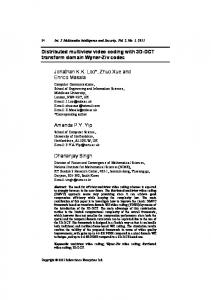
PSNR vs spatial correlation level ρS for systems with 8 cameras (C = 23.5 M bps, r = 11.7 M bps, TD = 5, and ρT = 0, Ballet sequence

build the φ matrix as explained in Sec. III. In the Appendix we provide some further details on the construction of the matrix. In short, the number of regions in which each frame is subdivided depends on both the video content and the correlation level. Thus, frames can be decomposed into different regions. In particular, each region is designed by a unique combination of correlated frames that are involved in the reconstruction at the decoder. In the temporal domain, the contribution of neighboring frames to each region is evaluated by comparing images from the same camera. More precisely, each frame is subdivided into regions, each of them can be reconstructed from previously acquired frames only if no motion occurs in these regions. As no motion estimation is employed at the source coding nor at the receiver in our system, only the fixed background contributes to the temporal extrapolation of missing frames. In the spatial domain, to evaluate the influence of each camera on the neighboring ones, we use DIBR techniques and calculate the number of pixels that can be estimated from neighboring views. This can be achieved by each camera with the information about its own depth map, and about the positions of the neighbor cameras. The overhead information required for this estimation thus corresponds to the information about the camera positions, which is generally of small size. As observed in [36], the exact value of the correlation level is however not a critical parameter in the scheduling optimization. Errors in the correlation evaluation, caused by a coarser estimation with a smaller overhead, does not have a significant impact on the scheduling policies. Thus, in the following, we assume a precise knowledge of the correlation information and we neglect the small overhead required to estimate the correlation level. Since we are interested in reconstructing all the views (at the clients), simulation results are provided in terms of mean PSNR, which is the PSNR averaged over all the frames of all views. This means that, even if some frames are decoded at high PSNR values, the average PSNR of the reconstructed scene might be in the low PSNR range in challenging transmission conditions. First, the PSNR of the reconstructed scene is evaluated from the rate-distortion model described in Sec. III-C. Then we validate our findings by experiments with actual reconstruction of the video frames at the decoder. The proposed algorithm has been compared to two baseline algorithms: a random allocation of the DUs (“Baseline RNDM”), whose distortion performance has been averaged over 1000 runs, and a scheduling solution where cameras priorities are defined a priori based on the joint entropy of the camera dataset as defined in [28] (“Baseline - Akyildiz”). In particular, the camera selection for the latter method is based on the spatial correlation that exists between views, while time correlation information is neglected. The camera priority is established as follows: the camera minimizing the overall distortion becomes the highest priority camera. Then, other cameras are included if they maximize the diversity (i.e., if they minimize the spatial correlation) with respect to the cameras that have been previously selected. We first provide results for a greedy optimization scenario (i.e., K = 1) and demonstrate the benefit of a correlation-aware scheduling optimization w.r.t. baseline algorithms. Then we depict the performance of foresighted optimization solutions, showing that low-complexity solutions lead to good performance when the optimization horizon is enlarged. B. Greedy Optimization We first analyze the performance of our algorithm in the case where the optimization horizon is limited to the next transmission time slot. We first study the importance of the knowledge of the correlation information in the optimization. Our optimization algorithm is evaluated in different conditions that depend on the type of correlation information considered in the scheduling decisions: i) “Correlation Known”, when the full correlation information is considered in the optimization; ii) “Space Corr Known”, when only the spatial correlation is considered; iii) “Time Corr Known”, when only the temporal correlation is used; iv) “No corr known”, when the scheduler completely ignores the correlation between frames.

12

Table I AVERAGE PSNR OF THE RECONSTRUCTED IMAGES FOR EACH CAMERA FOR SYSTEMS WITH 8 CAMERAS (ρS = 8, ρT = 3, C = 23.5 M bps, r = 11.7 M bps, AND TD = 5), FOR THE BALLET SEQUENCE MODEL . Optimization Method No Correlation known Correlation known Baseline - Akyildiz

1 24.95 26.19 22.28

2 25.32 26.26 23.07

3 26.97 24.13 24.87

Camera 4 27.44 28.08 24.52

view 5 26.88 26.23 24.64

6 26.69 25.18 25.84

7 25.80 26.87 23.84

8 25.26 26.18 22.55

27 26 25

PSNR

24 23 22 Correlation Known Space corr known Time corr known No corr known Baseline − RNDM Baseline − Akyildiz

21 20 19

0

1

2

3

4 ρ

5

6

7

8

s

Figure 6. model).

PSNR vs spatial correlation level ρS for systems with 8 cameras (C = 23.5 M bps, r = 11.7 M bps, ρT = 3, and TD = 5, Ballet sequence

We first study the gain that can be achieved when the correlation model is known by the scheduler. In the following figures, the PSNR of the reconstructed scene is evaluated from the rate-distortion model described in Sec. III-C. In the first experiments reported in Fig. 5, the temporal correlation between cameras is neglected both at the scheduler and at the decoder and we focus on the influence of the spatial correlation, which means that missing frames are reconstructed from neighboring views but not from previous frames. The performance of the scheduling algorithm is given as a function of the spatial correlation ρS (i.e., a function of the number of views that are considered to be spatially correlated) for systems with 8 cameras, a playback delay TD = 5, a constant encoding rate per camera of r = 11.7 M bps and a channel capacity C = 23.5 M bps4. This bandwidth constraint means that 2 only frames out of 8 can be allocated on the channel between each frame acquisition. First, we observe that the gain experienced by the algorithm using the spatial correlation information in the scheduling compared to the case in which all the correlation levels are ignored is substantial and this gain increases with the number of correlated frames (i.e., with ρS ). Thus, the knowledge of the spatial correlation is able to considerably improve the efficiency of the scheduling decisions. Moreover, the proposed algorithm outperforms both baseline algorithms. This means that the packet scheduling optimization leads to a better level of adaptation than the a priori camera selection technique in [28]. It is interesting to note that, by neglecting the correlation model (“No Correlation Known”) the performance becomes very bad and even worse than a random allocation solution. This means that, rather than choosing the scheduling based on wrong correlation information, it is better to completely ignore it. In the next experiment, temporal correlation is considered in the scheduling decisions. The PSNR quality is provided in Fig. 6 as a function of the number of spatially correlated cameras ρS for systems with 8 cameras, C = 23.5 M bps, r = 11.7 M bps and a temporal correlation ρT = 3 (i.e., each frame is considered to be correlated with the three previous frames of the same camera view). It can be observed that the algorithm using temporal correlation (“Time Corr Known”) is the closest one to the algorithm using all the correlation information (“Corr Known”). It has to be noted that all the results provided in the Fig. 6 have been evaluated considering temporal interpolation at the decoder. However, not all the algorithms include this information in the scheduling optimization. For example, the algorithm that only takes into account the spatial correlation information (“Space Corr Known”) is not able to outperform the baseline algorithm with random allocation. This means that, when views are highly correlated in both temporal and spatial domains, a partial information on the correlation does not always lead to a considerable gain in the scheduling optimization. In Table I, the average PSNR for the sequences reconstructed in the different camera views is provided for the same experiment. It can be observed that most of the reconstructed camera views achieve the highest PSNR with the correlation-aware scheduling algorithm. We now repeat similar experiments in a different camera configuration with only 4 views. In Fig. 7, the PSNR quality is 4 Note

that r = R[bpp] · SR [pixel per frame] · FR [f ps].

13

22

30 Correlation Known Space corr known Time corr known No corr known Baseline − RNDM

21.5

28 27

PSNR

21

PSNR

Correlation Known Space corr known Time corr known No corr known Baseline − RNDM

29

20.5

20

26 25 24 23

19.5 22 19 5.8

11.6

17.4 23.2 Encoding Rate [bpp]

29

21 5.8

34.8

11.6

(a) ρT = 0, ρS = 0.

17.4 23.2 Encoding Rate

29

34.8

(b) ρT = 2, ρS = 4.

PSNR vs encoding rate for systems with 4 cameras (C = 23.5 M bps, and TD = 5, Ballet sequence model).

Figure 7.

25

26

Correlation Known Baseline − RNDM No corr known

24.5

25.5 25

24

PSNR

PSNR

24.5

23.5

23

24 23.5 23

22.5 22.5

22

21.5

0

0.5

1

1.5 ρt

2

2.5

3

(a) PSNR vs temporal correlation information ρT for systems with 4 cameras (C = 23.5 M bps, r = 23.5 M bps, ρS = 2, and TD = 5). Figure 8.

Correlation Known Baseline − RNDM Baseline Akyildiz

22 21.5

2

3

4

5 ρs

6

7

8

(b) PSNR vs spatial correlation level ρS for systems with 8 cameras (C = 23.5 M bps, r = 11.7 M bps, ρT = 3, and TD = 5).

Reconstructed PSNR for systems with 4 and 8 cameras for different encoding rates and levels of correlation (Ballet sequence).

measured as a function of the encoding rate (C = 23.5 M bps, TD = 5). It can be observed that there is a tradeoff in the choice of the encoding rate, which varies with the level of correlation information used in the scheduling decisions. This tradeoff is the result of a source quality that increases with encoding rate, while the penalty due to the channel also increases with encoding rate, since more DUs are dropped at high rate for the same channel bandwidth constraint. If there is no known correlation neither in time nor space (i.e., ρS = 0, ρT = 0 in Fig. 7(a)), it is better to reduce the encoding rate, so that there is a chance of increasing the number of DUs allocated for transmission, hence the diversity of the information. On the contrary, when the correlation can be exploited both in time and space for frame interpolation (i.e., ρS = 4, ρT = 2 in Fig. 7(b)), the best encoding rate appears to be a medium rate (17 M bps). This means that, in this case, rather than scheduling all the frames at low rate (i.e., r = 5.8 M bps), it is better to transmit less frames but at higher rate and to exploit the correlation for the reconstruction of the missing ones. Finally, we confirm the above observations on experiments with a system that performs actual reconstruction of the video frames at the decoder. These results are provided in Fig. 8. The “Baseline-Akyildiz” performs better than a random scheduling most of the time, but it is in general outperformed by the proposed scheduling optimization, for almost all the values ρS of spatial correlation. These observations are in line with our previous results where the quality is measured with the R-D model of Sec. III. They confirm the benefits of including correlation information in the scheduling algorithm, even in a greedy scenario (K = 1).

14

Table II AVERAGE PSNR OF THE RECONSTRUCTED SEQUENCE FOR EACH CAMERA FOR SYSTEMS WITH 4 CAMERAS (C = 47 M bps, r = 23.5 M bps, AND TD = 5), FOR THE BALLET SEQUENCE MODEL . Optimization Method Exhaustive search algorithm Branch pruning strategy

Static Cameras ρS = 0, ρT = 2 ρS = 2, ρT = 2 K=3 K=5 K=3 K=5 24.39 24.54 26.50 26.65 24.39 24.52 26.47 26.63

Moving Cameras ρS = 0, ρT = 2 ρS = 2, ρT = 2 K=3 K=5 K=3 K=5 23.13 23.19 25.07 25.20 23.11 23.16 25.05 25.18

Table III AVERAGE PSNR OF THE RECONSTRUCTED SEQUENCE FOR EACH CAMERA FOR SYSTEMS WITH 4 CAMERAS (C = 47 M bps, r = 23.5 M bps, AND TD = 5), FOR THE B REAKDANCER SEQUENCE MODEL . Optimization Method Exhaustive search algorithm Branch pruning strategy

Static Cameras ρs = 0, ρt = 2 ρs = 2, ρt = 2 K=3 K=5 K=3 K=5 23.09 23.25 25.56 25.70 23.03 23.23 25.54 25.67

Moving Cameras ρs = 0, ρt = 2 ρs = 2, ρt = 2 K=3 K=5 K=3 K=5 24.18 26.73 24.45 26.92 24.18 26.70 24.43 26.91

C. Large Optimization Horizon We now provide results for a framework with foresighted optimization where scheduling policies are computed for several future time slots (K > 1). We have already shown above the gain of the proposed algorithm over the baseline ones from K = 1, so that we now limit the study to the proposed scheduling algorithm, and look at the gain of a foresighted scheduling policy with respect to a greedy optimization. First, we provide results where the quality is measured with the R-D model of Sec. III (no actual reconstruction of the video frames at the decoder). Then we validate our findings by experiments with actual reconstruction of the video frames at the decoder. For the branch pruning strategy in the trellis-based scheduling solution, we consider the number of survivor branches per time slot to be Ns = 2. The results are provided for both a static scenario, where cameras are fixed and the correlation level variations are due to video content, and a dynamic scenario, where cameras are allowed to move in time with a dynamic level of spatial correlation.The random movement of the cameras is simulated as follows. We assume a set of 2M possible positions that each camera can take. We start the simulation by randomly allocating each camera in one of the available positions. At each time slot, a camera is randomly selected for changing its position (it can randomly move to the neighboring position). The camera moves only if the chosen position is not already occupied by another camera; otherwise no movement is performed by the camera set at this time slot. Based on the position of the cameras, the correlation level is evaluated. This means that the correlation between two neighboring cameras can dynamically vary in time, accordingly with the camera movement. In particular, each view can always be reconstructed from the two neighboring ones, but if these two are far apart the portion of frame that can be reconstructed will be small. Moreover, we also assume that the correlation with the frame previously acquired in time is zero when there is a camera motion. Each result provided in the following solution has been averaged over 1000 simulations runs. We first compare the proposed sub-optimal scheduling algorithm with an optimal one. In particular, we randomly select a time instant t ∈ [1, 100] and assume that the scheduling history till the time instant t − 1 is known 5 . We are interested in optimizing the scheduling policy over a time horizon of K time slots with our trellis-based search technique and with an optimal solution, which exhaustively search for the best scheduling policy. Decoding quality results for the DUs acquired during the time interval under consideration. Results of the reconstructed distortion of the DUs acquired during the time instants [1, t] are provided in Table II and in Table III, for the Ballet and Breakdancer video sequences, respectively. Each value is averaged over 1000 random simulations for both static and dynamic scenarios with C = 23.5 M bps, r = 11.7 M bps, and TD = 5. It can be observed that, for both sequences, the difference between the branch pruning strategy and the exhaustive search method is negligible. This means that the pruning of the branches in the trellis-based optimization does not penalize significantly the performance, while it drastically reduces the computational complexity. We now provide results for the proposed foresighted scheduling optimization in dynamic scenarios. In Fig. 9, the modelbased reconstructed PSNR is given as a function of the number of optimization time slots K for systems with 4 cameras for several temporal correlation levels (r = 23.5 M bps, ρs = 2, C = r and C = 2r). For all the temporal correlation values ρt , we provide results for large K and we observe performance gains with K. Note that the distortion gain due to large K is sometimes marginal for two main reasons: i) the channel capacity is very limited and only few DUs can be scheduled compared to the total number of acquired DUs (Fig. 9(a) where the channel capacity is equal to the source rate of one camera only); ii) there are large levels of correlation so that the system performance is less sensitive to non-optimal scheduling decisions since most of the views will be reconstructed at a fair level anyway (see Fig. 9(b) when ρt = 3). In Fig. 10, the PSNR quality is provided as a function of the optimization horizon K for systems with 8 dynamic cameras (C = 47 M bps, r = 23.5 M bps, TD = 5, and ρs = 4) for both Ballet and Breakdancer video sequences. By increasing 5 The

scheduling history is randomly selected.

15

33.5

30

29

33 28

32.5 PSNR

PSNR

27

26

32

25 ρT=1 24

23

1

2

3

4

5

6

7

8

ρ =1

31.5

T

ρT=2

ρ =2

ρT=3

ρT=3

9

T

31

10

1

2

3

4

5

6

7

8

9

10

K

K

(a) C = 23.5 M bps

(b) C = 47 M bps

Figure 9. PSNR vs optimization horizon K for systems with 4 dynamic cameras (r = 23.5 M bps, TD = 5, ρs = 2, and Ns = 2, Ballet model sequence).

30.5

31.5

30

31

29.5

30.5 29

PSNR

PSNR

30 28.5

29.5 28

29 27.5

ρt=1

ρ =1 T

ρT=2 27

ρt=2

28.5

ρ =3

ρt=3

T

26.5

1

2

3

4

5

6

7

K

(a) Ballet sequence model.

8

9

10

28 1

2

3

4

5

6

7

K slots

(b) Breakdancer sequence model.

Figure 10. Model-based reconstruction PSNR vs optimization horizon K for systems with 8 dynamic cameras (C = 47 M bps, r = 23.5 M bps, TD = 5, ρs = 4, and Ns = 2).

the number of cameras from 4 to 8 but keeping the ratio between the channel constraint C and source rate r constant, the number of DUs that cannot be scheduled increases; this makes the selection of the best scheduling policy even more crucial. As expected, the quality gain for large optimization horizons gets more important in this case. Finally, in Fig. 11, experimental results are provided for systems with 8 dynamic cameras (C = 47 M bps, r = 23.5 M bps, TD = 5, and ρs = 4). The experiment is the same of Fig. 10 but the actual reconstruction of the scene is performed at the decoder. As already demonstrated for the greedy optimization results, the qualitative behavior of the experimental and model-based results is similar. In general we observe that, the larger the temporal correlation, the better the quality in the reconstruction since more past frames can be used in the reconstruction of a given frame. Furthermore, the experimental results confirm that increasing the optimization horizon improves the performance, as already observed in the results derived from the model-based results. From the simulation results, we can draw the following learnings. First, we have demonstrated that the temporal and spatial correlations that exist among acquired frames in a multiview scenario is a crucial piece of information in the optimization of the streaming strategy. When packet filtering is imposed by bottleneck channels, the packet scheduling strategy can drastically benefit from the knowledge of the correlation that exists between data units. We have also shown that a foresighted optimization strategy outperforms greedy optimizations in most cases. Moreover, the benefit of considering the correlation level in the packet scheduling algorithm increases in dynamic scenarios compared to static ones. The proposed algorithm is optimized in real time

16

24.3

26

24.2 24.1

25.5

24 23.9 PSNR

PSNR

25

23.8 23.7

24.5

23.6 24

ρt=1

23.5

ρ =1

ρt=2

T

ρ =2 T

ρt=3

23.4

ρ =3 T

23.5

1

2

3

4 K

(a) Ballet sequence.

Figure 11.

5

6

23.3 1

2

3

4

5

6

7

K

(b) Breakdancer sequence.

Reconstructed PSNR for systems with 8 dynamic cameras (C = 47 M bps, r = 23.5 M bps, TD = 5, ρs = 4, and Ns = 2).

and refined at each transmission opportunity, allowing to consider dynamic scenarios, in which both cameras positions and the level of correlation can vary in time. In addition, it is worth noting that i) when the level of correlation exists in both the time and space domains, knowing at least one of the two correlation levels leads to an improvement in the scheduling algorithm compared to the case where no correlation information is known; ii) the knowledge of the correlation level might help in selecting the best rate at which each camera should encode the images. In particular, the greater the level of correlation, the lower then number of views that needs to be allocated per acquisition time for optimal performance. Based on the above learnings, several possible research directions can be studied. The packet scheduling algorithm can be extended to source coding optimization problems, where the rate of each view could be adapted over time. It could also be extended to scenarios with unreliable channels. At large, the proposed framework can be used in different systems in emerging multiview video streaming applications, in which both spatial and temporal correlations represent crucial information for adapting the video delivery solution. VII. C ONCLUSIONS We have investigated the impact of frame correlation for the scheduling of packets in a multi-camera system. In particular, we have proposed both a novel RD model able to take into account the correlation level among cameras and a method to estimate the contribution that each camera can offer in the reconstruction of correlated views. Based on this model, we have proposed an optimization algorithm, which determines the packet scheduling policy by taking into account the channel capacity and both the temporal and spatial correlations among encoded frames. The proposed algorithm is able to adapt the transmission strategy to the level of correlation experienced by each camera. We have formalized a trellis-based optimization and we have proposed a suboptimal yet effective solution with a tractable complexity, based on effective pruning in a trellis representation. Simulation results have demonstrated the gain of the proposed method compared to classical resource allocation techniques. Finally, we have also demonstrated the robustness of foresighted optimization strategies. A PPENDIX φ M ATRIX C ONSTRUCTION We now provide further details on the construction of the φ matrix. The entire process is based on the subregions in which each frame is subdivided. In more details, the number of regions in which each frame is subdivided depends on both the video content and the correlation level. Thus, frames can be decomposed into different regions. Each region is designed by a unique combination of correlated frames that are involved in the reconstruction at the decoder. In the temporal domain, the contribution of neighboring frames to each region is evaluated by comparing images from the same camera. More precisely, each frame is subdivided into regions, each of them can be reconstructed from previously acquired frames only if no motion occurs in these regions. As no motion estimation is employed at the source coding nor at the receiver in our system, only the fixed background contributes to the temporal extrapolation of missing frames. In the spatial domain, to evaluate the influence of each camera on the neighboring ones, we use DIBR techniques and calculate the number of pixels that can be estimated from neighboring views. In Fig. 12, we provide an example to better explain how the φ matrix is constructed and what is the meaning of each element of the matrix. In the figure, we consider a scenario in which two cameras acquire the scene of interest. We are interested in

17

(a)

(b)

(c) Figure 12. Example in constructing the regions in which the frame Ft,1 is subdivided. (a) Regions of frame Ft,1 reconstructable from frame Ft,2 . (b) Regions of frame Ft,1 reconstructable from frame Ft−2,1 . (c) Regions of frame Ft,1 reconstructable from frame Ft−1,1 .

evaluating the matrix for the frame Ft,1 (depicted in the figure as a dashed-border box), knowing that Ft,2 , Ft−1,1 and Ft−2,1 are correlated to Ft,1 . In Fig. 12 (a)-(c) we show which parts of the frame Ft,1 can be reconstructed from Ft,2 , Ft−1,1 and Ft−2,1 , respectively. Regions that can be reconstructed (i.e., that are correlated) from the neighboring one are highlighted in grey in each subfigure. For example, from Fig. 12 (a), we observe that regions 3, 4, 6, and 7 of frame Ft,1 are correlated to frame Ft,2 . Thus, we can build a vector φ (v2) = [0 0 1 1 0 1 1]T that maps the spatial correlation between the two views into the reconstructable subregions. If we then look at a specific region, say for example region 1, we observe that the region is reconstructable from frame Ft−2,1 and Ft−1,1 but not from Ft,2 . So, we can notice that each region has a unique combination of frames that can be used for the reconstruction at the decoder. Note also that all the regions of each frame can be always completely reconstructed from the same frame. This means that the vector φ (v1) , which depicts the regions of Ft,1 that can be reconstructed from Ft,1 , corresponds to a unitary vector. Merging together all the vectors φ (v1) , φ (v2) , φ (t−2) , φ (t−1) , we obtain the following matrix   1 0 1 1  1 0 0 1    1 1 1 0    φ (v1) |φ φ (v2) |φ φ (t−2) |φ φ(t−1) ] =  φ 1,t = [φ (9)  1 1 1 1 .  1 0 0 0    1 1 0 1 1 1 0 0

18

φj,1,t }7j=1 , where φ j,1,t describes which of the neighboring frames can Recalling the notation that we used in Sec. III, φ 1,t = {φ contribute to the reconstruction of the region sj . From this matrix, we can notice that region 5 can be reconstructed only if the frame of interest (i.e., Ft,1 ) is received. Otherwise, the region cannot be reconstructed by any neighboring frame. As general intuition, the larger is the level of correlation between frames, the greater is the number of non zero elements in the matrix. R EFERENCES [1] W.-P. Yiu, X. Jin, and S.-H. Chan, “VMesh: Distributed segment storage for peer-to-peer interactive video streaming,” IEEE J. Select. Areas Commun., vol. 25, no. 9, pp. 1717 –1731, Dec. 2007. [2] G. Cheung, A. Ortega, and N.-M. Cheung, “Interactive streaming of stored multiview video using redundant frame structures,” IEEE Trans. Image Processing, vol. 20, no. 3, pp. 744 –761, March 2011. [3] T. Maugey and P. Frossard, “Interactive multiview video system with low complexity 2D look around at decoder,” IEEE Trans. Multimedia, 2013. [4] A. Kubota, A. Smolic, M. Magnor, M. Tanimoto, T. Chen, and C. Zhang, “Multiview imaging and 3DTV,” IEEE Signal Processing Mag., vol. 24, no. 6, pp. 10 –21, Nov. 2007. [5] “IEEE Standard for Information technology– Specific requirements Part 11: Wireless LAN Medium Access Control (MAC) and Physical Layer (PHY) Specifications,” IEEE Std 802.11-2012 (Revision of IEEE Std 802.11-2007), 2012. [6] J. T. Qunli Jia, Effective point coordination function in wireless LAN. U.S. Patent WO2004059913 A3, Nov. 11, 2004. [7] Cisco Systems Inc., Transport Diversity: Performance Routing (PfR). White Paper, Oct. 2009. [8] Texas Instruments Inc., Smart grid leverages ARM-based solutions to enable intelligent power consumption with a more robust end-to-end communication network. White Paper, Aug. 2012. [9] L. Zhou and H.-H. Chen, “On distributed multimedia scheduling with constrained control channels,” IEEE Trans. Multimedia, vol. 13, no. 5, pp. 1040 –1051, Oct. 2011. [10] H.-P. Shiang and M. van der Schaar, “Information-constrained resource allocation in multicamera wireless surveillance networks,” IEEE Trans. on Circuits and Syst. for Video Tech., vol. 20, no. 4, pp. 505 –517, April 2010. [11] D. Slepian and J. Wolf, “Noiseless coding of correlated information sources,” IEEE Trans. Inform. Theory, vol. 19, no. 4, pp. 471 – 480, Jul. 1973. [12] A. Wyner and J. Ziv, “The rate-distortion function for source coding with side information at the decoder,” IEEE Trans. Inform. Theory, vol. 22, no. 1, pp. 1 – 10, Jan. 1976. [13] Z. Xiong, A. Liveris, and S. Cheng, “Distributed source coding for sensor networks,” IEEE Sig. Proc. Mag., vol. 21, no. 5, pp. 80 – 94, Sept. 2004. [14] Y. Wu, V. Stankovic, Z. Xiong, and S.-Y. Kung, “On practical design for joint distributed source and network coding,” IEEE Trans. Inform. Theory, vol. 55, no. 4, pp. 1709 –1720, Apr. 2009. [15] S. Li and A. Ramamoorthy, “Networked distributed source coding,” in Theoretical Aspects of Distributed Computing in Sensor Networks. Springer Berlin Heidelberg, 2011, pp. 191–224. [16] E. Kurutepe, M. Civanlar, and A. Tekalp, “Client-driven selective streaming of multiview video for interactive 3DTV,” IEEE Trans. Circuits Syst. Video Technol., vol. 17, no. 11, pp. 1558 –1565, Nov. 2007. [17] G. Cheung, V. Velisavljevic, and A. Ortega, “On dependent bit allocation for multiview image coding with depth-image-based rendering,” IEEE Trans. Image Processing, vol. 20, no. 11, pp. 3179 –3194, Nov. 2011. [18] Y. Liu, Q. Huang, S. Ma, D. Zhao, and W. Gao, “RD-optimized interactive streaming of multiview video with multiple encodings,” Journal of Visual Commun. and Image Representation, vol. 21, no. 5, pp. 523 – 532, March 2010. [19] E. Kurutepe and T. Sikora, “Multi-view video streaming over P2P networks with low start-up delay,” in Proc. IEEE Int. Conf. on Image Processing, Oct. 2008, pp. 3088 –3091. [20] Z. Chen, M. Zhang, L. Sun, and S. Yang, “Delay-guaranteed interactive multiview video streaming,” in Proc. IEEE Int. Symposium on Circuits and Systems, May 2009, pp. 1795 –1798. [21] Z. Pan, Y. Ikuta, M. Bandai, and T. Watanabe, “User dependent scheme for multi-view video transmission,” in Proc. IEEE Int. Conf. on Communications, June 2011, pp. 1 –5. [22] J.-G. Lou, H. Cai, and J. Li, “Interactive multiview video delivery based on IP multicast,” Journal of Adv. MultiMedia, vol. 2007, no. 1, Jan. 2007. [23] N. Anantrasirichai, D. Agrafiotis, and D. Bull, “Distributed video coding for wireless multi-camera networks,” in Proc. IEEE Int. Conf. on Visual Information Engineering, Aug. 2008, pp. 67 –70. [24] N.-M. Cheung, A. Ortega, and G. Cheung, “Distributed source coding techniques for interactive multiview video streaming,” in Proc. Picture Coding Symp., May 2009, pp. 1 –4. [25] Z. Yang, W. Wu, K. Nahrstedt, G. Kurillo, and R. Bajcsy, “Enabling multi-party 3D tele-immersive environments with viewcast,” ACM Trans. Multimedia Comput. Commun. Appl., vol. 6, no. 2, Mar. 2010. [26] D. Bandari, G. Pottie, and P. Frossard, “Correlation-aware resource allocation in multi-cell networks,” IEEE Trans. on Wireless Commun., vol. 11, no. 12, pp. 4438–4445, Dec. 2012. [27] M. C. Vuran and I. F. Akyildiz, “Spatial correlation-based collaborative medium access control in wireless sensor networks,” IEEE/ACM Trans. Netw., vol. 14, pp. 316–329, Apr. 2006. [28] R. Dai and I. Akyildiz, “A spatial correlation model for visual information in wireless multimedia sensor networks,” IEEE Trans. Multimedia, vol. 11, no. 6, pp. 1148 –1159, Oct. 2009. [29] P. Wang, R. Dai, , and I. F. Akyildiz, “Visual correlation-based image gathering for wireless multimedia sensor networks,” in Proc. IEEE Int. Conf. on Computer Communications, Apr. 2011, pp. 746 –749. [30] Z. Liu, G. Cheung, and Y. Ji, “Distributed Markov decision process in cooperative peer recovery for WWAN multiview video multicast,” in Proc. IEEE Int. Conf. on Visual Communications and Image Processing, Nov. 2011, pp. 1–4. [31] K. M¨uller, P. Merkle, and T. Wiegand, “3D video representation using depth maps,” Proc. IEEE, vol. 99, pp. 643–656, April 2011. [32] T. A. Cover and J. A. Thomas, Elements of Information Theory, 1st ed. New York, NY, 10158: John Wiley & Sons, Inc., 1991. [33] P. Chou and Z. Miao, “Rate-distortion optimized streaming of packetized media,” IEEE Trans. Multimedia, vol. 8, no. 2, pp. 390 – 404, April 2006. [34] [Online]. Available: http://research.microsoft.com/en-us/um/people/sbkang/3dvideodownload/ [35] L. Toni, T. Maugey, and P. Frossard, “Multi-view video packet scheduling,” arXiv:1212.4455, vol. abs/1212.4455, 2012. [36] ——, “Correlation-aware packet scheduling for multi-camera streaming,” in Proc. IEEE Int. Packet Video Workshop, May 2012, pp. 77 –82.