Jul 29, 2005 - Continual coordination is a process that occurs over time, and as such deals with ...... [13] Dana S. Nau, Stephen J. J. Smith, and Kutluhan Erol.
Multiagent Coordination by Extended Markov Tracking Zinovi Rabinovich Jeffrey S. Rosenschein School of Engineering and Computer Science Hebrew University, Jerusalem, Israel {nomad, jeff}@cs.huji.ac.il
ABSTRACT We present here Extended Markov Tracking (EMT), a computationally tractable method for the online estimation of Markovian system dynamics, along with experimental support for its successful contribution to a specific control architecture. The control architecture leverages EMT to simultaneously track and correct system dynamics. Using a widespread extension of the Markovian environment model to multiagent systems, we provide an application of EMTbased control to multiagent coordination. The resulting coordinated action algorithm, in contrast to alternative approaches, does not eliminate interference among agents, but rather exploits it for purposes of synchronization and implicit information transfer. This information transfer enables the algorithm to be computationally tractable. Experiments are presented that demonstrate the effectiveness of EMT-based control for multiagent coordination in stochastic environments.
Categories and Subject Descriptors I.2.8 [Problem Solving, Control Methods, and Search]; I.2.11 [Distributed Artificial Intelligence]: Multiagent systems; I.2.11 [Distributed Artificial Intelligence]: Coherence and coordination
General Terms Algorithms
Keywords Control, Planning, Coordination, Multiagent Systems, Markovian Environment
1.
INTRODUCTION
Imagine a team of robots sent into a danger zone on a search and rescue mission. Sophisticated machines, they carefully navigate uneven ground, mapping their way, monitoring for sudden changes in the environment or each other. They find an injured person, and two of the robots carry the victim out on a stretcher, careful to keep it as steady as possible.
Permission to make digital or hard copies of all or part of this work for personal or classroom use is granted without fee provided that copies are not made or distributed for profit or commercial advantage and that copies bear this notice and the full citation on the first page. To copy otherwise, to republish, to post on servers or to redistribute to lists, requires prior specific permission and/or a fee. AAMAS’05, July 25-29, 2005, Utrecht, Netherlands. Copyright 2005 ACM 1-59593-094-9/05/0007 ...$5.00.
This scenario may require the solution of many hard problems for a robotic agent: planning and control in a stochastic domain, data fusion and data mining, model learning; and all of these, even when individually solvable, are made much harder by the need for continually coordinated performance. The latter, if not handled properly, will be easily hindered by unintentional interference between the team members, observational noise, and uncertainty about the environment and its response to actions. Continual coordination is a process that occurs over time, and as such deals with the exhibited behavior of the system over time— that is, the system dynamics, rather than the system state at a single point in time. In teamwork, the dynamics that the system is supposed to exhibit may be known, and the coordination task is to ensure that those dynamics are brought about. This means continual tracking of the system dynamics, detection of deviation from the ideal dynamics, and choice of action in an attempt to correct the deviation. A tracking mechanism that we introduce in this paper, called Extended Markov Tracking (EMT), allows efficient observation-based estimation of the dynamics exhibited by a system. By incorporating EMT as a predictor in a control schema, we achieve the simultaneous tracking and correction of system dynamics for a single agent. Extending the environment model used by EMT-based Control to include multiple agents, we obtain a coordinated action algorithm for stochastic domains. The resulting coordinated action algorithm, in contrast to alternative approaches, does not eliminate interference among agents, but rather exploits it for purposes of synchronization and implicit information transfer. As a result, it becomes computationally feasible to carry out the coordinated choice of actions.
1.1 Overview of the Paper The rest of the paper is organized as follows. We first discuss the background and connections of the proposed algorithm, to relate it to and distinguish it from other research, in Section 2. We then provide technical details of our algorithm for the tracking of system dynamics, in Section 3. Application to control and modification for coordinated action is presented in Section 4, and experimental performance results of EMT Control follow in Section 5. We expand discussion of the technique in Section 6, and then present conclusions in Section 7.
2. RELATED WORK EMT Control has many connections to other research in the literature, which we will review in this section. Most of these connections can be classified into one of two main groups: (1) those related to Information Theory, and (2) those related to Decision Theory.
2.1 Information Theory Connections System dynamics has long been a subject of inquiry in information theory [7]. That field mainly deals with Markovian dynamics, where the current system state probabilistically depends on a finite history backwards in time. These dynamics (and we also adopt this description) are represented by a conditional distribution, and describe the way information is transmitted through a noisy channel. One of the major tasks of information theory is to find a source coding to maximize the rate and accuracy of information transfer. Among the most recent works on the subject are those of Tishby et al. [19, 20], which propose a novel method for distributional clustering and relevant quantization. An elegant theoretical schema is built for preserving maximum relevant information, when it has to be transmitted via a third party. For example, image-based face recognition has two stages: image “compression” into features, then face recognition based on the features. [20] provides an exact, self-consistent set of equations that allow optimal creation of feature coding, so that information relevant to face recognition will be maximally preserved in the derived features. Later work [19] provides a practical algorithm for developing the feature set itself, also through a widely applicable mathematical construction. Notice that source coding can be seen as open loop control: preset source code defines what kind of dynamics the overall system will exhibit as time goes to infinity. Control with Extended Markov Tracking (EMT), which we present here, exploits similar mathematical tools and notation. It also deals with the system state passing through the noisy channel of a state transition function. However, the task it faces differs significantly in several respects. First, EMT Control has no ability to directly predetermine the way that the system state will be distributed; instead, EMT Control has only a limited set of actions that will influence the channel noise, which (in turn) will continually change the system state distribution. Second, EMT Control does not have the luxury of infinite time. Exhibited dynamics must stay within tight bounds at all times, not only in the limit. An information-theoretic approach to coordinated control was also used by the research group of Durrant-Whyte [3, 10]. In their work, multi-robot sensor systems are explored within the framework of decentralized data fusion. As a consequence, control becomes a function of predicting information gain from an action, and choosing the best prospect. Allowing non-frequent exchange of observation information, a successful control schema is developed. However, it is important to note that the goal of their systems is information itself. In our work, we tend toward more general systems, where information is only a key to better control, not the ultimate goal. Also, as will be shown in the experiment set of Section 5, the coordinated action control proposed in this paper does not use explicit information exchange, but rather exploits implicit information transfer through the environment, which further generalizes the approach.
2.2 Decision Theory Connections Another related branch of research is Markov Decision Problems (MDPs), and their extensions to multiagent domains. MDPs also have at their core a Markovian model of system dynamics. However, they do not deal directly with ideal system dynamics. Instead, MDPs see them as a reward function, dictating how much gain or cost would be incurred if the system would move from one state to another. The idea is that maximizing the average reward (accumulated over time, or accumulated in a discounted fashion over time) [14] requires the system to follow and exhibit the ideal dynamics. Solving fully observable MDPs, where it is possible to determine completely the system state from observations, is relatively
simple. However, Partially Observable MDPs (POMDPs) are hard to solve [4, 12, 2]. There have been several extensions of the Markovian environment model to multiagent settings. They preserve the MDP economic perspective, and attempt solutions mostly based on reinforcement learning techniques (e.g., [11, 15, 1]). However, agent actions interfere with one another, creating observational noise, so multiagent MDPs are at least as hard as POMDP, even if explicit communication is available at no cost. If, in addition, communication is limited or is subject to cost, the exact solution of multiagent MDPs becomes exceptionally hard. Computational complexity reaches NEXP in all system parameters, and what is even worse, the problem is inapproximable—good approximate solutions have equally high complexity [15, 17]. The classical way to reduce this complexity is to eliminate the interference between the agents or to break the problem into smaller parts, e.g., [4, 9]. These approaches regard inter-agent dependencies created by system feedback as a hazard. A refreshingly neutral work in this sense is that of Wolpert et al. [23, 24]. That research views inter-agent interference as a side effect of their activity, and attempts to align them, providing alternative targets for each agent to achieve. This in turn improves system performance. The EMT-based coordinated action algorithm presented in this paper goes further, and views interference between agents as an asset. The algorithm exploits that interference to implicitly transfer information between the agents through the environment. This ability should indeed be an important feature of any coordinated action control algorithm. It allows us, together with a well-formed mathematical apparatus, to compel the system to exhibit the desired dynamics, while investing computational effort only polynomial in the system description.
3. EXTENDED MARKOV TRACKING Determining, from observations, the behavioral trends of an environment during interaction with it is known to be a hard problem. It is universally treated by complex models that require significant amounts of data and involve a large computational burden [18, 5, 16]. However, usually interaction is either short-lived and discrete in time or, although internally complex, exhibits simple external trends. Thus, a simple Markovian model will often be sufficient for our needs.
3.1 Model A Markovian environment is described by a tuple < S, A, T, O, Ω, s0 >, where: • S is the set of all possible environment states; • s0 is the initial state of the environment (which can also be viewed as a distribution over S); • A is the set of all possible actions applicable in the environment; • T is the environment’s probabilistic transition function: T : S × A → Π(S). That is, T (s� |a, s) is the probability that the environment will move from state s to state s� under action a; • O is the set of all possible observations. This is what the sensor input would look like for an outside observer; • Ω is the observation probability function: Ω : S × A × S → Π(O). That is, Ω(o|s� , a, s) is the probability that one will observe o given that the environment has moved from state s to state s� under action a.
In many current approaches, including previously mentioned MDPs (Section 2), “tracking” means a continual estimation of the system state as seen through the distortion of observations. We believe this approach is insufficient, since it actually disregards the continual nature of tracking. Rather than understanding where the system is moving, it is of greater importance to know how it is moving. In other words, instead of tracking the system state, one needs to track the way the system changes, i.e., the dynamics of the system. This is what makes Extended Markov Tracking (EMT) so wellsuited for coordinated action choice. Unlike other approaches that have to be adapted to the task, EMT concentrates directly on the subject of coordination: system dynamics.
3.2 Tracking of Dynamics EMT tracks the system dynamics by continually performing a conservative update of a system dynamics estimate expressed as a mapping P D : S → Π(S). After every development epoch of the system, the EMT algorithm searches for an explanation dynamics D that can account for the change in system state. An explanation that differs least from the old dynamics estimate then becomes the new estimate. The distance between old and new system estimates is measured by EMT using the Kullback-Leibler (KL) divergence function [7]: DKL (p�q) =
� x
p(x) . p(x) log q(x)
From the information theoretic point of view, this is the price one will have to pay for using distribution q to encode a source distributed by p. In our case, the old dynamics estimate is the encoding we use, while the new dynamics estimate stands in for the true source distribution. In a sense, KL divergence would measure the “regret” of using an old estimate in light of new evidence and a new estimate of the system dynamics. Conservative update dictates the minimization of this regret. However, to complete the measure and system dynamics tracking, one has to maintain one auxiliary kind of information: beliefs about the current system state. Initial beliefs are given by the definition of the environment tuple. Assume that at some stage we believe p ∈ Π(S), and we obtain an observation o ∈ O after action a. Then we can update our beliefs using the Bayesian formula: p˜(s) ∝ Ω(o|s, a)
�
T (s|a, s� )p(s� ).
s�
Notice that, although action is present in computations of the state estimator, it serves as an input to the procedure, and not as an unknown parametric component. Given that we keep track of our beliefs about the environment state, we can do the same with regard to the observed dynamics. Our prior beliefs in this case might obviously depend on the domain, but in the absence of any other preference, one commonly accepted prior belief is the uniform distribution. That is, we assume at the beginning that anything can happen in the environment with equal likelihood. The other popular alternative is a ‘static’ environment, that is, the assumption that the system state does not change. Thus, we can formally define EMT update as follows. Denote old beliefs about the exhibited system dynamics by P D(s� |s), and � the new beliefs by that explain the change in system state �D(s |s), � D(s� |s)p(s), where p(·) and p˜(·) are, respecthat is p˜(s ) = s
tively, the old and the new estimations of the system state. D is the
conservative update we seek if it exists: D(s� |s) = arg min �DKL (Q(s� |s)�P D(s� |s)) p(s) � Q(s |s)
s.t. � ∀s� p˜(s� ) = Q(s� |s)p(s) s � Q(s� |s) = 1 ∀s s�
The optimization problem above is convex, and can be solved efficiently in time and space complexity polynomial in the description of the system, e.g., numerically by gradient descent or alternatively by an internal point algorithm. Notice that the Kullback-Leibler extension for Markovian dynamics, �DKL (Q(s� |s)�P D(s� |s)) p(s) , can also provide failure detection for controllers. This is used in a two-level control architecture into which we incorporate EMT, as described below in Section 4.
4. CONTROL WITH EMT The control framework we use consists of two continually interacting layers: • The strategic layer is concerned with the following question: given a high level goal, what kind of system dynamics will suffice to achieve it; • The tactical layer has no concern whatsoever with the high level goal. Rather, it attempts to ensure that the system dynamics of the changing state indeed match the one desired by the strategic layer. Failure of the tactical layer is reported back to the strategic layer, forming a closed control loop. Although the strategic/tactical paradigm is evident in many old and new planners and controllers [8, 21, 13], it may be desirable, as we have done, to shift responsibilities to the tactical layer, which typically is present only in a degenerate sense within existing approaches. In this work, we propose to implement the tactical layer by means of Extended Markov Tracking as presented above, and to base action selection directly on the system dynamics. Thus the strategic/tactical architecture becomes related to a paradigm of cooperation/coordination. Cooperation (working together, the strategic layer) dictates the ideal system dynamics r : S → Π(S) (or so called tactical target), and the coordinated action selection algorithm (the tactical layer) provides a means to achieve it. Formally, the EMT-extended tactical solution, or EMT Controller, operates as follows. Denote by H(¯ p, p, P D) the EMT procedure of obtaining the optimal explanation for transition between belief states p and p¯ with respect to the dynamics-prior P D. Denote as pt the belief about the system state at time t, and P Dt the beliefs about the exhibited system dynamics at time t. Also, let Ta be the environment transition function restricted to action a (Ta p thus becomes a matrix applied on a vector). Then, the action of choice in the EMT Controller is: a∗ = arg min �DKL (H(Ta p, p, P D)�r) p . a
While the overall EMT Controller algorithm may be written as follows: 0. Initialize estimators: • the system state estimator p0 (s) = s0 ∈ Π(S);
• system dynamics estimator P D0 (¯ s|s) = prior(¯ s|s) Set time to t = 0.
The EMT Control loop operates almost unchanged in the multiagent setting, with only a slight modification to accommodate the fact that each agent contributes only a part of the joint action. N � Let A = Ai ; also, denote by pt,i the belief of agent i at time t i=1
1. Select action a∗ to apply using the following computation: • For each action a ∈ A predict the future state distribution p¯at+1 = Ta ∗ pt ; • For each action, compute Da = H(¯ pat+1 , pt , P Dt );
about the system state, and by P Dt,i the beliefs of agent i at time t about the exhibited system dynamics. Then each agent 1 ≤ i ≤ N performs the following: 0. Initialize estimators: • the system state estimator p0,i (s) = s0 ∈ Π(S); • system dynamics estimator
∗
• Select a = arg min �DKL (Da �r) pt .
s|s) = prior(¯ s|s) P D0,i (¯
a
2. Apply the selected action a∗ and then receive an observation o ∈ O. 3. Compute pt+1 due to the Bayesian update. 4. Compute P Dt+1 = H(pt+1 , pt , P Dt ). 5. Set t := t + 1, goto 1. In essence, the tactical algorithm above utilizes extended Markov tracking both to guide its action selection, and to ensure that the exhibited behavior indeed concurs with the given preference mapping r : S → Π(S).
4.1 Coordination by EMT Control Consider now a cooperative multiagent system with no communication between the agents. In such systems, performing coordinated action requires the utilization of implicit data transfer through the environment to synchronize agents. This can be done by the EMT Control scheme: each agent will estimate the exhibited system dynamics based on its own observational data, choose the bestfitted joint action, and perform its part in it. If agent effects on the system are correlated, EMT will provide the means for information transfer and synchronization. However, to apply EMT Control we first need to modify the Markovian environment model to include multiple agents. We adopt the approach taken by Tambe [15], where the system environment N N is described by a tuple < S, {Ai }N i=1 , T, {Oi }i=1 , {Ωi }i=1 , s0 >, where: • N is the number of agents in the system; • S is the set of all possible environment states as before; • s0 is the initial state of the environment; • Ai is the set of all possible actions applicable in the environment by agent i; • T is the environment’s probabilistic transition function: T : S × A1 × · · · × AN → Π(S). That is, T (s� |�a, s) is the probability that the environment will move from state s to state s� under the joint action �a = (a1 , . . . , aN ); • Oi is the set of all possible observations available to agent i; • Ωi (oi |s� , �a, s) is the probability that the agent i will observe oi ∈ Oi given that the environment has moved from state s to state s� under the joint action �a = (a1 , . . . , aN ).
Set time to t = 0. 1. Select action a∗ ∈ A to apply using the following computation: • For each action a ∈ A predict the future state distribution p¯at+1,i = Ta ∗ pt,i , where Ta is the transition function limited to action a; • For each action, compute Da = H(¯ pat+1,i , pt,i , P Dt,i ); • Select a∗ = arg min �DKL (Da �r) pt,i . a
2. From the selected actions a∗ = (a1 , . . . , aN ) apply action ai ∈ Ai , and receive an observation oi ∈ Oi . 3. Compute pt+1,i due to the Bayesian update. 4. Compute P Dt+1,i = H(pt+1,i , pt,i , P Dt,i ). 5. Set t := t + 1, goto 1.
5. EXPERIMENTAL DATA To demonstrate the operational qualities of the proposed EMT Control loop and its extension to multiagent coordination, we designed several experiment sets. A single-agent scenario that was used to test the EMT Control loop was based on the Drunk Man Walk problem, and allowed us to evaluate EMT Control performance. Since no truly tactical alternative solution currently exists, we used a standard POMDP solver [6] as a point of reference for our technique. A multiagent scenario involved two agents with no explicit communication, nor any direct effect on each other’s actions. However, the system response correlated the actions of the agents in a nontrivial way, providing an implicit means of information exchange.
5.1 Single Agent Case: Drunk Man Walk The Drunk Man Walk domain (Figure 1) is a classic example for Markov chain discussions: a man stumbles along a path between his home and nettle bushes, making random steps left (home) and right (bushes). The setup was modified to allow stochastic control—actions can be applied to tilt the probability balance between left and right steps, but the potential number of steps taken each move was greater than one (in our experiments, 1/4 of the path could be traversed in a single epoch). In addition, the true position of the man was veiled by the observation set—which is the same size as the set of possible positions. The observation probabilities essentially just “blur” the
Figure 1: Drunk Man state transition diagram. α is subject to action effect. system state. The task was to keep the man as far away as possible from home and nettle bushes alike. The classic delayed reward schema, where one is rewarded if the man reached the middle of the path, was translated into a transition preference matrix for our tactical solution. The comparison was done based on the distribution of distance from the path midpoint. In the experiment set, which resulted in the data shown in Figure 2, the preference over the state transitions was set to � 1+ x ¯ = � n+1 � 2 P (¯ x|x) = Z(x) otherwise Z(x) where Z(x) is a normalization factor. The classical POMDP solution used the same preference as a reward function, and attempted to accumulate as large a reward as possible over a preset number of steps. The observation set was the same size as the system state set, and probabilities were preset so that observations were equally distributed over the immediate neighborhood of the man’s true position. 1.1
1
0.8 Cumulative probability
111111111111111111111 000000000000000000000 000000000000000000000 111111111111111111111 111111111111111111111 000000000000000000000 Figure 3: Springed bar setting Formally, the system state is described by the positions of the two agents on the bar, S = [1 : dmax ]2 , where dmax is the length of the bar in “steps”, and the initial state in our experiment set was unbalanced as follows: s0 = (1, dmax + 1). The action sets are 2 Ai = {lef t, stay, right}, and the transition probability is set according to the simplified physics of motion as described above. We considered two observation schemes: 1. Oi = S = {all positions of the two agents}, Ω1 = Ω2 and creates uniform noise over the immediate neighborhood of the real joint position of agents.
0.9
2. Oi = [1 : dmax ] and represents the position of the observing agent. Ωi creates a uniform noise over the immediate neighborhood of the observing agent’s real position.
0.7
0.6
0.5
0.4
0.3
0.2 EMT POMDP 0.1
At each time step of the system, each agent has the choice of three actions: moving left one step, moving right one step, or staying put. Every movement of an agent has a non-zero probability of failing, and the probability is biased by the inclination of the bar. Specifically, an uphill motion has less probability of succeeding than if the bar were level, and a downhill motion has greater probability of succeeding than if the bar were level. Notice that the bar inclination itself depends on the current agent positions on the bar, thus creating a correlation between the effects of the agent actions, and providing a means for implicit information transfer between the agents.
0
1
2
3 Distance from goal position
4
5
6
Figure 2: Drunk Man: Distance from mid-point The tactical solution, our EMT Controller, outperformed the classical POMDP solution. Figure 2 shows cumulative probability that the Drunk Man will be away from the global goal position—midpoint along the path. The EMT Controller places the Drunk Man closer to the midpoint more frequently, and as a consequence will gain more profit compared to the classical POMDP solution.
5.2 Multiagent Case: Springed Bar Balance Consider a long bar whose ends rest on two equivalent springs, and two agents of equal mass standing on the bar. Their task is to shift themselves around so that the bar levels, as shown in Figure 3.
In the first observation scenario, agents converge to a symmetric position around the ideal center of mass (given that the springs and masses are equal, this ends up being the center of the bar), in spite of the stochastic nature of the environment. An example run can be seen in Figure 4. Average deviation with confidence bars is shown in Figure 5. In the second observation scenario, where agents have only noisy observations of their own position, an interesting kind of behavior is created by the control algorithm. Agents cannot step off the bar, and any action that attempts to do so fails. That, together with the symmetric nature of the problem, drives the agents toward a “focal point”, or equilibrium point, where each agent occupies the far end of the bar, thus balancing it. Somewhat surprisingly, the agents’ positions in the second observational scenario quickly converge to this focal point. What is even more interesting is the way that the agents arrive at the equilibrium. The initial state of the system places one agent at the far end of the bar, while the second stands quite close to the middle. The intuitive way to move towards the focal point position (the two far ends of the bar) would be for the second agent to move away from the center, while the first agent stays put, especially since the agents do not see one another. Recall, though, that the bar would be tilted, slowing the second agent down. EMT Control
16
16 Agent 1 Agent 2 Center of Mass
14
12
Position on the bar 1≤ pos ≤ dmax=15
Position on the bar 1≤ pos ≤ dmax=15
14
10
8
6
10
8
6
4
4
2
2
0
5
10
15
20 Time step
25
30
35
0
40
Agent 1 Agent 2 Center of Mass
12
5
Figure 4: Multiagent observational scenario I.
10
15
20 Time step
25
30
35
40
Figure 6: ‘Helping’ behavior
2
16 1.5
Agent 1 Agent 2 Center of Mass
1
Position on the bar 1≤ pos ≤ dmax=15
Deviation −confidence bar value *10
4
14
0.5
0
−0.5
−1
12
10
8
6
4 −1.5
2 −2
10
20
30
40
50 60 Time Step
70
80
90
100
Figure 5: Multiagent observational scenario I. Deviation from the ideal center of mass accounts for that, and many runs of the experiment move the first agent towards the middle of the bar, thus helping the second agent to reach its destination; only then does the control algorithm return the first agent to the original far end position. This behavior can be seen in the example run in Figure 6. However, because of observational noise the first agent sometimes overshoots, moving too far to the middle. EMT Control of the second agent detects that overshoot and recalls the second agent towards the center of the bar, allowing the first agent to correct its mistake. At its extreme, this behavior can cause “switching”, where the agents actually switch their relative positions, passing each other at the center as shown in Figure 7. However, EMT Control agents in all of our 100 experimental runs managed to balance the bar, as shown by the statistical data in Figure 8.
6.
DISCUSSION
Several interesting questions arise from our experimental results, beyond their immediate scope. For example, what could explain the fact that EMT Control outperformed the POMDP solution with respect to accumulated reward, the very success measure for which
0
5
10
15
20 Time step
25
30
35
40
Figure 7: ‘Switching’ behavior
the POMDP solution was designed? One plausible explanation lies with an interesting observation about the Bellman-Ford equation on which all (PO)MDP solutions are ultimately based. The equation has two significant parts: the first is the accumulation of the reward, and the second is the averaging over possible system developments. POMDP solutions, despite their limited knowledge of the true system state, center around the reward that enters the equation. On the other hand, EMT acknowledges that, because of limited system state information, we may not obtain the best reward possible, and in a sense sees it as inevitable and out of the reach of its own control. Instead, EMT concentrates on its influence on the distribution over which the “reward” will be averaged, and evidently prevails. Another interesting question concerns tactical target design. We find that, compared to (PO)MDP reward scheme design, tactical target composition is rather intuitive. Once again we turn to Drunk Man as an example domain. If we retain the reward scheme as before (recall we “designed it” to keep the Drunk Man as close to the center of the path as possible), but allow complete state observability, we can use a fully observable MDP to solve the problem. The
0.25
1.5
1
0.2
0.5
Probability
Deviation
0.15 0
0.1 −0.5
0.05
−1
−1.5
10
20
30
40
50 60 Time Step
70
80
90
100
0
1
2
3
4
5
6 7 8 9 Position along the path
10
11
12
13
Figure 8: Deviation from the ideal center of mass in multiagent observational scenario II.
Figure 10: Drunk Man state distribution under EMT control
MDP solution is quickly obtained by dynamic programming. However, the chosen reward scheme does not make the MDP solution behave as required. The Drunk Man moves randomly, and although motion trends can be affected, he is unlikely to stay put. This leads the MDP solver to a controlled fall solution: the Drunk Man will leave the middle of the path anyway—and by applying maximal force will make sure of where he ends up, then apply the inverse to make sure he comes back. An example of the distribution over positions along the path can be seen in Figure 9. It shows that the MDP solution forces the Drunk Man away from the vicinity of the path’s middle for a large portion of the time. Yet, the intuition that failed for MDP works correctly for EMT control, which created a Gaussian-like position distribution around the path center (Figure 10).
rated it into a control architecture. The resulting EMT Controller allowed us to simultaneously track and correct the exhibited system dynamics; the Controller was in turn applied to coordination in a multiagent domain. The online nature of EMT, and its intrinsic connection with system interactions, allowed us to leverage the correlation between the effects that agent actions have on the system dynamics. In effect, EMT Control has created implicit communication through the environment. Correlated behavior was demonstrated in the second observational scenario of our multiagent experiment set, in the absence of explicit communication. Since the EMT Control scheme takes time polynomial in the size of the system description, applying it to multiagent domains significantly reduces the computational complexity of coordination in these domains. In fact, EMT Control is polynomial in all parameters, other than the number of agents in the system. The experimental data collected so far demonstrates the efficiency of the approach both in single and multiagent domains. It would be worthwhile to compare EMT Controller performance to other multiagent solutions, e.g., the MiniMax-Q algorithm and neural networks. However, although we have made some progress in this direction within the single agent environment, for multiagent scenarios it would be quite difficult to construct a uniform benchmark problem for the comparison of inherently different algorithmic approaches. To explore EMT Control applicability, we plan to expand our experimental investigation, and create a spectrum of problems characterized by different degrees of interdependency between agent effects on the system, as well as general system volatility. In addition, it will be important to test EMT-based control in multiagent domains with available but limited explicit communication, and to investigate its performance with respect to other bounded resources.
0.35
0.3
Probability
0.25
0.2
0.15
0.1
0.05
0
1
2
3
4
5
6 7 8 9 Position along the path
10
11
12
13
8. REFERENCES Figure 9: Drunk Man state distribution under MDP solution control
7.
CONCLUSIONS AND FUTURE WORK
We have introduced an on-line tracking mechanism of system dynamics, called Extended Markov Tracking (EMT), and incorpo-
[1] Daniel S. Bernstein, Robert Givan, Neil Immerman, and Shlomo Zilberstein. The complexity of decentralized control of Markov decision processes. Mathematics of Operations Research, 27(4):819–840, 2002. [2] Vincent D. Blondel and John N. Tsitsiklis. A survey of computational complexity results in systems and control. Automatica, 36(9):1249–1274, September 2000.
[3] Frederic Bourgault, Alexei A. Makarenko, Stephan B. Williams, Ben Grocholsky, and Hugh Durrant-Whyte. Information based adaptive robotic exploration. In IEEE/RSJ International Conference on Intelligent Robots and Systems (IROS), 2002. [4] Craig Boutilier, Thomas Dean, and Steve Hanks. Decision-theoretic planning: structural assumptions and computational leverage. Journal of Artificial Intelligence Research (JAIR), 11:1–94, 1999. [5] Hung H. Bui. A general model for online probabilistic plan recognition. In Proceedings of the 18th International Joint Conference on Artificial Intelligence (IJCAI), pages 1309–1315, 2003. [6] Anthony R. Cassandra. POMDP solver software. http://www.cassandra.org/pomdp/code/index.shtml, 2003. [7] Thomas M. Cover and Joy A. Thomas. Elements of information theory. Wiley, 1991. [8] Richard E. Fikes and Nils J. Nilsson. STRIPS: a new approach to the application of theorem proving to problem solving. Artificial Intelligence, 2:189–208, 1971. [9] Claudia V. Goldman and Shlomo Zilberstein. Decentralized control of cooperative systems: Categorization and complexity analysis. Journal of Artificial Intelligence Research (JAIR), 22:143–174, November 2004. [10] Ben Grocholsky, Alexei Makarenko, and Hugh Durrant-Whyte. Information-theoretic coordinated control of multiple sensor platforms. In IEEE International Conference on Robotics and Automation (ICRA), Taipei, Taiwan, 2003. [11] Michael L. Littman. Value-function reinforcement learning in Markov games. Journal of Cognitive Research, 2:55–66, 2001. [12] Omid Madani, Steve Hanks, and Anne Condon. On the undecidability of probabilistic planning and related stochastic optimization problems. AI Journal, 147(1-2):5–34, July 2003. [13] Dana S. Nau, Stephen J. J. Smith, and Kutluhan Erol. Control strategies in HTN planning: Theory versus practice. In Proceedings of the 15th National Conference on Aritificial Intelligence (AAAI/IAAI), pages 1127–1133, 1998. [14] Martin L. Puterman. Markov Decision Processes. Wiley-Interscience Publication, 1994. [15] David V. Pynadath and Milind Tambe. The communicative multiagent team decision problem: Analyzing teamwork theories and models. Journal of Artificial Intelligence Research (JAIR), 16:389–423, 2002. [16] David V. Pynadath and Michael P. Wellman. Probabilistic state-dependent grammars for plan recognition. In Proceedings of the 16th Conference on Uncertainty in Artificial Intelligence (UAI), pages 507–514, 2000. [17] Zinovi Rabinovich. Non-approximability of centralized control in distributed systems. Master’s thesis, Computer Science, Hebrew University, Jerusalem, Israel, January 2002. [18] Patrick Riley and Manuela Veloso. Recognizing probabilistic opponent movement models. In A. Birk, S. Coradeschi, and S. Tadokoro, editors, RoboCup-2001: The Fifth RoboCup Competitions and Conferences. Springer Verlag, 2002. [19] Noam Slonim and Naftali Tishby. Agglomerative information bottlenecks. In Advances in Neural Information Processing Systems (NIPS-12), pages 617–623. MIT Press, 2000. [20] Naftali Tishby, Fernando C. Pereira, and William Bialek. The
[21]
[22]
[23] [24]
information bottleneck method. In The 37th Annual Allerton Conference on Computation, Control and Computing, pages 368–377, 1999. Manuela M. Veloso, Jaime Carbonell, Alicia Prez, Daniel Borrajo, Eugene Fink, and Jim Blythe. Integrating planning and learning: The PRODIGY architecture. Journal of Experimental and Theoretical Artificial Intelligence (JETAI), 7(1):81–120, 1995. Richard Washington. Markov tracking for agent coordination. In Agents-98: The Second International Conference on Autonomous Agents, pages 70–77, 1998. D. H. Wolpert. Product distribution field theory, 2003. D. H. Wolpert, K. R. Wheeler, and K. Tumer. Collective intelligence for control of distributed dynamical systems. Europhysics Letters, 49(6):708–714, 2000.