While using correctly the wireless multicast advantage, these protocol focus ... problem of finding a minimum cost multicast tree in wired network (i.e., without.
Chapter 5
Multicasting, geocasting, and anycasting in sensor and actuator networks Arnaud Casteigts, Amiya Nayak and Ivan Stojmenovi´c School of Information Technology and Engineering, University of Ottawa, 800 King Edward, Ottawa, Ontario K1N 6N5, Canada.
Abstract This chapter reviews the scenarios where a given message is sent from a single source to possibly several destinations. These scenarios can be subdivided into multicasting, geocasting, multiratecasting, and anycasting. In multicasting, a given message must be routed from one node to a number of destinations whose locations may be arbitrary and spread over the network. Geocasting destinations are all nodes located in a given geographical area. Multiratecasting is a generalization of multicasting, where regular messages are sent from a source to several destinations, possibly at a different rate for each destination. Finally, in an anycasting scenario, a source must send a message to any node among a given set of destinations, preferably only one. Each of these scenarios corresponds to a typical use case in sensor and actuator networks.
5.1
Multicasting
In a multicasting task, the same message is routed from one single source node to a fixed number of destinations whose locations are potentially scattered in the network. In the context of sensor and actuator networks, this routing scheme is
1
CHAPTER 5. XCASTING
2 A3
S
A2 A1
Figure 5.1: Multicasting from a sensor S to actuators A1 , A2 , A3 usually applied by sensors to report their data to several actuators (as illustrated on Figure 5.1). More formally, given a graph G = (V, E), a source s ∈ V and a set of destinations D ⊆ V , the multicast problem consists in finding a set of relay nodes R ⊂ V such that s ∪ F ∪ R is connected in G. The main idea behind multicast is to try to reduce R as much as possible (share a maximum of the links to send as few duplicate packets as possible). In most of the algorithms, this path sharing consists in building an overlay tree whose root is the source and leaves are destinations (destinations may also act as relay nodes, though). This is however not always the case, some algorithms rather build a mesh overlay which better tolerate the failure of links, thanks to redundancy. Also, when the positions of destinations are known beforehands, the multicast task can be achieved without using any overlay structure. In this latter case, the paths may also form trees or meshes, but these structures are built on the fly and not memorized. The present section reviews these different solutions.
5.1.1
Non-geographic multicast
A number of multicast protocols (DVMRP [DC90], MOSPF [Moy94], CBT [BFC93], PIM [DEF+ 94]) were first proposed in the context of Internet, and more generally IP networks. These protocols were specifically designed for wired and infrastructured network and are not relevant in the context of wireless sensor networks. The main reason is that they do not make use of the broadcast nature of the wireless medium. Indeed, in a wireless context, the transmission of a message from one node to any number of its neighbors can be achieved in one single emission. This property, called the wireless multicast advantage, implies to modify both the routing strategy and the metrics used to measure its efficiency: summing the total number of hops (edges) does not precisely reflect the efficiency of a wireless path, whereas counting the number of transmissions do it better. Another important concern, which is not addressed by the aforementioned protocols, is the one of minimizing the energy consumption. This criterion is not very relevent in an infrastructured network, but it of utmost importance in the networks where devices are self-powered, such as sensor and actuator networks.
CHAPTER 5. XCASTING
3
A number of multicast protocols taking into account the wireless multicast advantage have been proposed this past decade in the area of Mobile Ad hoc Networks (or MANETs). These protocols are usually classified according to two criteria: whether they are proactive or reactive, and whether they rely on trees or meshes. Proactive protocols compute and maintain routing tables ahead of time, whereas reactive (also called on-demand ) protocols establish the given route once explicitely needed, and do not maintain it afterward. The reactive approach performs generally better than the proactive in dynamic topologies, since maintaining proactive routing information in this context is expensive. Regarding the shape of the routing structures, tree-based protocols build a tree from the source to the destinations, while mesh-based approaches intentionally add redundancy by considering additional links in order to tolerate topological changes. Meshes are generally considered more robust than trees, but induce a higher overhead. Examples of tree-based schemes are AMRIS [WT99] (which proactively builds a shared multicast tree among a set of sources and destinations), MAODV [RP00] (which extends the well-known AODV reactive protocol by adding an activable multicast mode on top of paths built by AODV), or ADMR [JJ01] (which constructs an overlay multicast tree from each source to its destinations, parts of the trees being possibly shared by different sources). Examples of meshbased approaches include CAMP [GLAM99] (an extension of the proactive Core Based Trees protocol that adds redundant links) or ODMRP [LGC99] (a reactive protocol that computes several paths among sources and destinations). Some protocols, such as AMROUTE [XTML02], combine tree- and mesh-based approaches. Finally, some protocols such as MCEDAR [SSB99] or the one in [JS02] rely on a backbone structure. While using correctly the wireless multicast advantage, these protocol focus more on finding quick and robust multicast paths than on minimizing the energy consumption. This is mainly due to the fact that building an energy efficient multicast tree consumes additional time, which is critical in highly dynamical contexts, because an energy-efficient tree may no longer exist by the time it is computed. In near-static scenarios such as sensor and actuator networks, however, taking the time to build an energy efficient path is relevant. The problem of finding a minimum cost multicast tree in wired network (i.e., without considering the wireless advantage) is known to be NP-complete, even when every link has the same cost (this problem is similar to the Steiner tree problem, where the weights of all edges are equal to 1 [Kar72]). In wireless network, where the purpose is to minimize the number of retransmissions instead of the number of hops, this problem is still NP-complete, as proven in [RGS05]. Some heuristics have been considered, such as in [RS07]. However, as for the protocols described before, the routing strategy considered here rely on an overlay structure that covers the whole network. Constructing and maintaining such structure may be very costly in message overhead and does not scale well in large networks. When the positions of nodes are known, a better and more efficient routing can be achieved.
CHAPTER 5. XCASTING
5.1.2
4
Geographic multicasting
The general idea behind geographic routing is to use the positions of nodes to achieve efficient routing without requiring the construction and maintainance of global routing structures such as trees and meshes. This comes from the observation that the very measurements of sensors do not usually have a proper meaning unless associated with the corresponding geographical information. Hence, assuming the availability of position information on sensors is not a so strong hypothesis. Geographic unicast has been discussed in the Chapter 4 of this book. We review in this section the protocols that extend geographic routing to multicast scenarios. First are briefly mentioned geographical, but non-localized, protocols, which are not optimal in the context of sensor and actuator networks. We review then some protocols that are both geographical and localized. One of the first non-localized geographical multicast protocol, LAM [JC98], still makes use of broadcast messages, and is therefore not practical in large wireless sensor networks. Another protocol from the same authors, DDM [JC01], combines several unicast data tables to set up multicast data forwarding. The management of these tables requires additional overhead and makes it limited to small multicast groups. Finally, a protocol proposed in [MYT04] uses position information to build a geographically aware multicast tree that aims at minimizing the number of links. However, as discussed before, minimizing the number of edges (hops) does not exploit the one-to-many nature of the wireless medium (wireless multicast advantage). Additionally, this protocol builds a global overlay structure, which is costly to maintain and does not scale in large networks. The best advantage of geographic routing is certainly to avoid the necessity of building and maintaining a global routing structure, while enabling the use of localized and stateless protocols where all the information needed to route a message is carried inside it and the selection of next relay neighbors is done on the fly at each hop. Such routing requires that every node knows 1) its own position using either GPS-like positioning service, or virtual coordinates (see Chapter 4 Section 7, or [Nic04]), 2) the position of its direct neighbors (using a beaconing scheme), and 3) the positions of the destinations (actuators) to report to, by using a location service (topic discussed in Chapter 8). The multicast protocols reviewed below (GMP, PBM, GMR, HGMR, and HRPM) are such protocols. GMP [WC06] works as follows: at every hop, the current forwarding node builds a virtual multicast Steiner tree, rooted in itself, whose leaves are the real destinations. This tree is obtained by merging the destinations by pair, creating a virtual node to represent them. The process goes recursively until no reduction is profitable. Based on this tree and on the positions of local neighbors, the destination set is then possibly split into several groups, and a neighbor is chosen to serve each group at the next hop. To deal with void areas while forwarding to a subgroup of destinations, the protocol proposes to use a normal unicast face routing (see Chapter 4 Section 5, or [BMSU99]), where the destinations of the group are all replaced by a single point, being the
CHAPTER 5. XCASTING
5
average of their geographic locations. The main disadvantage of GMP lies in the heuristic it uses to build the Steiner tree. Indeed, it calculates the virtual nodes by merging only two nodes at a time, which may lead to wrong position estimations, especially if the destinations are scattered in the network or if they are surrounding the source node. Another protocol, PBM [MFWL03], was not initially designed for sensor networks. However it fulfills the criteria of localized-ness and limited network overhead. This protocol is a generalization of the Greedy-Face-Greedy principle (see Chapter 4 Section 5, or [BMSU99]) to multi-destination contexts. It relies on a trade-off between individual shortest paths for each destination and overall cost minimization, according to a chosen balance parameter λ. More precisely, in each step, the current forwarding node evaluates each possible combination C of next forwarding neighbors using a function f (C) = λN +(1−λ)D where N is the ratio of selected nodes among the total number of neighbors, D is the sum of all remaining distances from these neighbors to destinations (in proportion to the sum of distances from the current node), and λ is a value between 0 and 1. If the best subset of neighbors is a single node, then that node is the only relay for all the destinations. If a combination with several nodes is selected, then each of these nodes will further take care of a different part of the destinations. When no advance can be provided toward one or more destinations, a variant of face routing is used for these destinations, while greedy forwarding continues toward the others. The main problem with this approach is determining the optimal value for λ, as no single value is the best for all scenarios. An additional issue in dense network or for large multicast groups (large number of destinations) is that the algorithm evaluates all possible association combination between destinations and neighbors (whose complexity grows exponentially with the two factors). GMR [SRLS07] is another adaptation of Greedy-Face-Greedy (GFG) to multicast scenarios. The high-level adaptation of GFG is similar to the one of PBM: when a forwarding node cannot find any neighbor providing an advance toward some of the destinations (i.e., a local optimum is reached), those destinations are put in a list called the multicast face-list, and face routing is started for them. If a current forwarding node, in face routing, happens to be closer than the previous local optimum for a given destination, then this destination is removed from the face-list and added to the greedy-list (greedy routing is resumed for this destination). Note that the current node may select a same neighbor to serve in the two modes simultaneously (for different destinations), in which case a single message containing both information is transmitted. While similar to PBM for the high-level strategy, GMR significantly differs concerning the selection of the forwarding neighbors. In order to solve the complexity problem due to evaluating all the possible combinations, GMR consider an initial default combination, where each destination is individually served by the most convenient neighbor (i.e., the neighbor that provides the highest advance toward it). This leads to a set of destination subsets (or partitioning) P = {M1 , M2 , . . . , M|P | }, where each subset corresponds to destinations being served by the same neighbor. An example scenario
CHAPTER 5. XCASTING
6 d1
d2
n1
c
Results of the merging process: P2 = {{d1 , d2 , d3 , d4 }}, with {d1 , d2 , d3 , d4 } to be server by n2 .
n2 n3
Initial partitioning: P1 = {{d1 , d2 }, {d3 , d4 }}, with {d1 , d2 } to be served by n1 and {d3 , d4 } by n3 .
d3
The two subsets have been merged after comparing cost over progress ratios of P1 and P2 .
d4
Figure 5.2: Example of routing decision by GMR is given in Figure 5.2, where a current node c groups together the destinations d1 and d2 (with respect to n1 ), and d3 and d4 (with respect to n3 ). Once the initial partitioning is built, GMR optimizes it by merging the subsets, by pairs, as long as such merge is possible and profitable. To compare several partitionings, the protocol evaluates them according to the concept of cost over progress ratio (see Chapter 4 Section 3, or [KNS05] for general definitions), where cost is the number of selected nodes, and progress is the overall reduction of remaining distances to destinations (assuming the more appropriate neighbor for each subset). In the example of Figure 5.2, GMR evaluates the initial partitioning P1 , and the partitioning resulting from the merge, P2 . In this scenario, using only n2 gives a slight distance penalty, while reducing the cost by half. As a result, the merge is profitable and done. In more complex scenarios where several merges are possible, GMR evaluates all of them, applies only the most profitable, then evaluates again. While GMR solves the main drawbacks of PBM, it still has the disadvantage that the header of every packet contains information about each destination of the packet. Hence, the encoding overhead in each packet is function of the number of destinations, which become unacceptable if this number grows too large. HRPM [DPH08] is a recent protocol that tackles this problem by constructing a hierarchy to serve the destinations. This hierarchy is achieved by geographically dividing the network into cells, where the destinations register and unregister as they move in the network. Thanks to a sophisticated management of these registrations (described later), the source can obtain the list of all the cells that contain at least one destination, and then send the packet to these cells without caring about which particular destination is inside which particular cell. Each cell then forwards the packet to the destinations inside. Actually, a three or four level hierarchy levels can be used, but the authors showed that this two level hierarchy is sufficient to support up to 5800 destinations (with respect to keeping a moderate ratio of header length over data size). The main advantage of this protocol is to guarantee that the per-packet overhead is never more than a desired constant ω. To ensure this property, the dimensions of the cells are determined according to ω and to the size of the multicast group. As a consequence, each multicast group defines a particular space partitioning and
CHAPTER 5. XCASTING
7
cell management. We describe now how the cell management works. The protocol assumes that each multicast group has a unique identifier, and that each potential destination is aware of all the multicast groups it belongs to. This allows all the destinations of a same group to recreate the same local representation of the network division. Thanks to a common geographic hashing function, the identifier of each multicast group can be mapped into a particular location in the network, called the Rendezvous Point (RP), and into a particular location in each cell, called the Access Point, as illustrated in Figure 5.3. For AP x
AP x
AP x
AP x
AP x
AP x RP
AP x
AP x
AP x
AP x
AP x
AP x
AP x
AP x
AP x
AP x
x
Figure 5.3: Geographical division of the network, as shared by all the nodes of a same multicast group.
the sake of simplicity, we will first consider that both RP and APs are real nodes located at the expected locations (this is actually false, but helps the comprehension). Each time a destination moves, it reports its new location to the AP of its cell. When the underlying cell changes, the destination unregister from one AP, and register to the other. These memberships are reported by the APs to the RP. When a node wants to send a packet to a given multicast group, it first contacts the RP of this group (thanks to the group identifier and to the geographic hashing function), which sends back the list of cells containing at least one destination. Upon receiving this list, the sending node builds a virtual tree exclusively composed of the corresponding APs, except for the root (itself), and sends the data down the tree (using geographic unicast between each parent and child in the tree). Once the message reaches an AP, another set of geographical unicasts is used to reach the final destinations. The role of the RP, and of each AP, is actually played by the node that is the closest to the corresponding locations, and a special management is locally involved when one of the closest nodes changes. Keeping the AP and RP virtual locations allows to consider them as stationary nodes. For both unicast levels (source to APs, and APs to destinations), the unicast protocol that is used is an adaptation of Greedy-Face-Greedy, which slightly modifies the face routing mode to deal with virtual destinations such as the APs or the RP (the modification comes to turn
CHAPTER 5. XCASTING
8
around and select the closest node). HRPM has several advantages. In addition to the limited encoding overhead, it does not require an external location service, and has a very small group management cost (mainly due to the fact that RPs and APs are stationary locations). However, it is sub-optimal regarding the communications. Indeed, it uses a set of unicasts to go down the tree, which may imply at the greedy level to send several times the same message between the same nodes, and does not consider the wireless multicast advantage. HGMR [KDHS08] is an adaptation of HRPM dedicated to relatively dense and static networks (such as sensor and actuator networks). The general idea behind HGMR is to integrate the design concepts of GMR and HRPM, that is to provide both forwarding efficiency and scalability to large networks. As a recall, transmission of data with HRPM goes from the source to the APs (down a virtual tree of APs), then from each of these APs to the corresponding destinations. GMR’s has the highest gain when the multicast member density is large (the benefits of broadcasting is maximized), while in sparse networks, its advantage over unicast is mitigated by its encoding overhead (because all destinations are included in the header). Thus, for the transmission from the source to the APs, whose density is expected to be low, HGMR still uses unicast. But within each cell, where destinations are potentially closer from each other, it uses GMR’s cost over progress ratio multicast algorithm to select the next relay nodes at each hop. If the number of destinations inside a cell is too large to include all of them in the header, then the geographical decomposition can be adjusted consequently. Hence, the use of GMR within each cell instead of HRPM’s unicast-based forwarding strategy helps to reduce the number of transmissions. Another drawback of HRPM was that the hash function could result in the RP being very far from the source. For this reason, HGMR uses a hash function that generates positions within a square in the center of the whole region, which limits the worst cases.
5.2
Geocasting with guaranteed delivery
In a geocasting task, one source node sends a message to all the nodes located in a given geographic region, as illustrated in Figure 5.4. In the context of sensor and actuator networks, this operation is usually applied from an actuator node to all the sensor located in a region of particular sensing interest, this region having possibly different shapes (circular, oval, rectangular, etc.). This message could carry for example a request for immediate data from any sensor in the region, or inform the sensors about a new location to regularly report to, or give any other instruction that relates to the given region. Geocasting could be used for example to monitor the pollution at given locations around a factory (e.g. near the river), or successively requesting the sensors along a moving object trajectory (e.g. tracking the progression of an animal in a forest). Note that geocasting in these cases represent only the request leg, and does not concern the way the data are reported in the reverse direction.
CHAPTER 5. XCASTING
9
Figure 5.4: Example of geocasting As for the other routing principles (e.g. broadcasting, multicasting, or anycasting), a geocasting task can be greatly improved by preliminary putting in sleep mode all the sensor nodes that are not useful to the task, i.e., not used to connect the target region, nor to cover it. Such preliminary steps have been discussed in Chapter 3. We present below a review of geocasting protocols that are applicable to wireless sensor and actuator networks. These protocols generally assume that nodes know their own positions and the positions of their neighbors.
5.2.1
Geocasting without guaranteeing delivery
For most of the protocols, the task of geocasting consists in two major stages: the first is to reach one node in the targeted geographic region, and the second to inform the other nodes in the region, starting from this node. A simple solution is to route the message from the source to any node in the region using a greedy geographic protocol, and then to use blind flooding (each node inside the region retransmits exactly once) to reach the other nodes, as illustrated Figure 5.5. S N
Figure 5.5: Geocasting seen as the combination of unicasting and flooding Several localized protocols were proposed on this basis (a review of them is available in [Sto06]). Regarding the first stage, all these algorithms are based on a greedy advance, which is restricted to a virtual area delimitation between the source (or current node) and the target region, as illustrated by dashed
CHAPTER 5. XCASTING
10
limit 3 lim
it 1
limit 2
Figure 5.6: Disconnected geocasting region is an obstacle to guarantee the delivery lines in Figure 5.6. Examples of such restricted area include the space between tangents from the current node to the target region boundaries (limit 1 ), the rectangle containing the source and the target region (limit 2 ), or simply the area offering any physical progression to the target (limit 3 ). These methods inherently do not guarantee the delivery to the region when no route exist within the restricted area. For example, if the dotted nodes in Figure 5.6 were absent from the topology, then no route would be found despite the fact that there exist another one going round above. This problem can be solved by using the GreedyFace-Greedy (GFG) principle to reach the region (see Chapter 4, Section 5, or [BMSU99]). A simple geocasting protocol, proposed in [SRL99], makes use of GFG to route toward the region, and once inside, performed a flooding within the region. While this algorithm guarantees the delivery to at least one node in the region (under the assumption of an ideal MAC layer), it does not guarantee that all the nodes inside the region will get the message (second stage). Indeed, as shown in Figure 5.6, the sensors that cover a given geocast region may not necessarily be connected inside it, even if the coverage is complete (due to possibly different sensing and communication radii, or obstacles). They can be connected by nodes outside the region, though. The next paragraphs review three geocasting solutions that guarantee the delivery to all the nodes inside the region (provided they are indirectly connected to the source).
5.2.2
Geocasting based on traversing faces that intersect boundary
We call internal (resp. external) border node a node that is inside (resp. outside) the region and has at least one neighbor outside (resp. inside) the region in the considered planar subgraph. In [SH04] an algorithm was proposed that uses the GFG algorithm to forward the packet toward the region, and then activates a perimeter mechanism to guarantee delivery to all nodes inside the region. However, as shown in [Sto06], this mechanism does not actually guarantee delivery,
CHAPTER 5. XCASTING
11
S M
O
J
N K
I G
H W
C
F
D
A
B
E
Figure 5.7: Traversing faces that intersect boundaries although very similar to the following algorithm, that does. During the first stage, the source node sends the message toward geocasting region using GFG, which guarantees that the region is reached if connected to the source. Once at the region, three different behaviors are defined for nodes upon reception, depending on which node receives and which node sends. 1. If the receptor node is inside the region, then it retransmits the message in a broadcast fashion. This is done only the first time it receives this message (further copies are ignored). If this node is an internal border node, then it includes in the message an instruction for its external border neighbors, asking them to initiate right-hand face traversals (see case 2 below). 2. If the receptor node is an external border node that receives the message from one of its internal border neighbors, then it initiates a right-hand face traversal to explore the external continuation of each edge that is shared with an internal border neighbors. Further messages coming from any of its internal border neighbors are then ignored. 3. Contrarily to the protocol in [SH04], if the receptor is an external border node and the emitter is a node being outside the region, then it does not ignore the message (even if it has already performed the step in case 2), and forwards the message along the same face as received. This latter step is necessary to guarantee the delivery in some particular cases. All these operations are illustrated by the scenario in Figure 5.7. To start, source node S uses GFG to reach the region, which is done at N . According to
CHAPTER 5. XCASTING
12
case 1, N initiates a flooding inside the region, and node M initiates a righthand face traversal along the external continuation of edge N M (note that in the particular case where the external node get the message before the internal node, it is not necessary to wait for an instruction in order to start the face traversals). This face traversal reaches I, which ignores the message because already received it from the inside. Meanwhile, node K initiates the right-hand face traversal continuing IK. This traversal travels around the region (via node H) until coming back at J. Node O initiates a face traversal continuing the edge JO, which closes the loop at N . In the meantime, the first flooding from N has reached node W , which gave an instruction to A to start a face traversal continuing W A. This traversal ends up at node C (which retransmits). Node B starts the face traversal with respect to CB, reaching F (which ignores if already received from C, retransmits otherwise). Finally E starts a face traversal going back to A. At this point, the algorithm from [SH04] would terminate. Case 3 is applied by A to continue the face traversal and reach node D. A last face traversal closes the loop at W , which ignores the message. In some cases, guaranteeing the delivery implies to visit the whole network. This would have been the case if the dotted round edge between H and G did not map to a real set of connected nodes. Then, the face traversal would have turned around the other side of the network (the reader can imagine the face traversal turning around node H, reaching back M , then passing by the source S, reaching back M again, then traveling until G, turning around it, and finally reaching J).
5.2.3
Geocasting based on depth-first search traversal of face tree
Another geocasting algorithm that guarantees delivery to all the nodes in the region was proposed in [BMSU01]. Similarly to the previous protocol, it does not require any memory to be left at nodes, and needs only to carry some small amount of information with the messages. The protocol consists in applying GFG to route toward a node inside the region, and then to explore all the faces being located inside, or intersecting the region. This exploration, detailed later, is based on the fact that the set of edges that compose any face can be totally ordered by the edges’ relative positions to a given reference point in the plane. Based on this ordering relation, faces can be associated with one another to form a face tree whose root is the face containing the reference point. Then, the region can be entirely visited by performing a depth-first search among this tree of faces. The whole process must be applied on a planar subset of the network (e.g. the Gabriel Graph, see Chapter 4 Section 5). Given a face f and a point p located outside of the face, the set of edges of f can be totally ordered according to their distance to p (actually the distance of the closest point to p in the edge). In case of ties, this total order can be turned strict by considering additional comparison keys based on geometrical properties. Based on the ordering, each face (except the one containing p) can be associated with one of its own edge, called entry(f, p), being the closest to p. Now, if we consider that each entry edge is on the boundary of two different
CHAPTER 5. XCASTING
13
15 17
19
14 12
16
10
13
18
N
11
9 8
1
p
20 2
3
4
6
7
5
Figure 5.8: Face tree traversal faces, then these edges define a hierarchy of faces (and thereby an implicit tree of faces) such that for each face f but the one containing p, parent(f, p) is the face f 0 6= f having entry(f, p) among its edges. The algorithm works as follows: once the region is reached at one node N by the GFG protocol, this node selects a nearby geographical point p located inside any adjacent faces (which by definition are in the region, or intersect it). This face becomes the root of the face tree. The face tree is then constructed during the geocasting operation, it is in fact the geocasting operation. Starting from the face containing p, at N , the algorithm will visit the entire face, but, before passing each edge, it checks if this edge is an entry edge for the opposite face (the method for this checking is discussed in the next paragraph). If this is the case, then the current face traversal is interrupted in order to visit the child face. This process goes recursively until no child face is found, at which point the traversal of the parent face resumes (at the other endpoint of the entry edge). In order to limit the visit to the geocasting region, entry edges are defined only for faces that are located in the region, or intersect it. The algorithm is illustrated on Figure 5.8. In this figure, the thick path arriving at N from the outside stands for the first routing stage (e.g. Greedy-Face-Greedy protocol), the continuous dashed line corresponds to the depth-first traversal of the face tree through the whole region, starting at N , and ending at N . The faces are numbered in the sequencial order of their visit. Finally, entry edges are represented by dashed black edges, while the corresponding parent/child relations are coded by gray dotted arrows. Since the algorithm visits all the faces of the face tree (which is composed of all the faces intersecting the region, or being inside), it must necessarily visit all the nodes in these faces, and consequently all the nodes in the region. However, the algorithm suffers a hidden cost: in order to know whether a given edge is an entry edge for the opposite face, that face must be visited. This gives the
CHAPTER 5. XCASTING
14
algorithm a considerable message overhead. One possibility to mitigate this problem would be to determine entry edges only once for all the network, at the starting time, and memorize them on their endpoint nodes (assuming no topological changes afterwards). This implies that a common reference point p is agreed at the deploying time, and that the algorithm is modified to deal with geocasting regions that possibly do not contain p. Let us assume a first step where the message is routed from the geocasting source to any node inside the region (if the source is not already inside it); let s0 be this node. If p is inside the region, then geocasting may proceed by backtracking from s0 to p using parent links, and then running the normal depth-first search algorithm from p. If p is outside the region, then the algorithm can backtrack from s0 toward p, but stop as soon as a node outside the region is reached, say p0 . From p0 , a face traversal is made along the edges outside the region, which corresponds in Figure 5.8 to the external parts of the dashed ride. Along this perimeter, each entry edge (they are known) begins a separate depth-first search traversal, which together visit every face in the region. As with the original version, this algorithm works only if the geocasting region is convex. Assume for example a crescent ’C’ shape with p located near one of the two ends of the shape. The faces at the other end may have parent faces that are outside the region, and thereby may not be visited. This problem could be solved by a similar perimeter traversal, where all entry edges will be detected and induce a separate depth-first search. Another general optimization for this algorithm could be to work on a well chosen subset of the nodes, namely a connected dominating set (or CDS for short, see Chapter 2 for details). More precisely, we could first find a CDS among the nodes in the region, and then reduce the face tree traversal to these nodes only. By definition, every non-CDS node is at a distance 1 from a CDS node. As a consequence, it is sufficient that only the CDS nodes retransmit in order to reach all the nodes. A face traversal scheme based on connected dominating sets was proposed in [DSW02] to optimize the face mode of GFG. However, such optimization has never been proposed in the context of geocasting and face tree traversal. For illustration purposes, Figure 5.9 shows the same topological scenario depicted on 5.8, with the only difference that face tree traversal is performed on a CDS of the nodes inside the region. Here, the face tree is composed of two faces only: the root, containing p, and one child face. The light gray color depicts non-CDS nodes (and their edges), while normal colors depict the CDS nodes (and the edges between them).
5.2.4
Geocasting based on multicasting to the region entrance points
Another strategy to guarantee the delivery was proposed in [Sto04] and is based on the concept of entrance points. An entrance point (also called external border node in the previous subsection) is a node which is located outside the target region but has at least one of its neighbors inside it. The strategy consists in reducing the geocasting problem to the problem of reaching every such entrance
CHAPTER 5. XCASTING
15
2
N
1
p
Figure 5.9: CDS-based face tree traversal point, from which intelligent flooding can be initiated to reach the connected nodes inside the region. Let R be the transmission radius, assumed identical for every node. It can be observed that any entrance point is necessarily (by definition) at a distance ≤ R from the region border. It is then possible to reach all entrance points by using geographic multicasting to well chosen areas around the region. These locations, called entrance zones, must be determined such that: 1. any entrance point necessarily belongs to an entrance zone, which implies that the union of all entrance zones must surround the region with a width larger than R. 2. if a node inside any zone retransmits a message, then any other node inside the same zone must receive it. This property ensures the possibility to reach all potential entry points in a zone from any of the nodes in it. The associated requirement is that entrance zones must have a diameter smaller than R. As illustrated on Figure 5.10, these two constraints cannot be respected together if a single layer of zones is considered (both measures in Fig. 5.10(a) are incompatible). The exact construction of entrance zones to satisfy these criteria actually depends on the shape of the geocasting region. If the geocasting region is a rectangle, for example, then the entrance zones may be composed of two layers of squares of length R/2, or better, composed of rectangles where one dimension (the one perpendicular to the region) is R/2 and the other dimension is as large as possible, provided the zone’s diameter does not exceed R (as illustrated in Fig. 5.10(b)). Another example that considers a circular geocasting region is provided in [Sto06]. Once all entrance zones are determined by the source, a geographical multicast task is initiated from the source toward the ’centers’ of all zones using a
CHAPTER 5. XCASTING ≥R
16 ≥R
≤R
≤R
(a) One-layer entrance zones
(b) Two-layer entrance zones
Figure 5.10: Layering of the entrance zones protocol such as GMR (see Section 5.1). Note that what is called ’center’ here can actually be any point inside the zone. Once the multicast is started, the routing paths can split to serve the destinations optimally. For each destination, the process stops when any node inside the corresponding zone is reached, or if a loop in recovery mode is observed (which means the destination zone is empty or disconnected from the rest of the network). In the case where a node is reached, then this node retransmits once in order to reach all the potential entry points located in the same zone, and then these points, if any, initiate an intelligent flooding within the target region. Some ideas of optimizations for this protocol are proposed in [Sto04]. For example, several nodes on a path can collectively conclude that a zone (or a set of zones) is empty, and thereby prevent full loops in recovery mode. Another possible optimization is to force nodes to wait for a while between reception and retransmission, during the multicast task, in order to merge potential routing assignment received by different neighbors. Also, the fact that several flooding operations of the region can be triggered by different entrance zones at different times, requires to adjust timeouts and traffic memorization to somewhat larger values than in regular flooding tasks, in order to ensure that an already received message will be recognized and not retransmitted. Note that this time delay may be important due to the possible use of recovery mode by the multicast protocol. The main problem of this protocol is obviously the overhead induced by empty zones. Indeed, if we do not consider the optimizations discussed above, then each empty zone may trigger a possibly large face traversal within the network, and even if part of the loops can be avoided, the protocol is still expected to incur large communication overhead in sparse networks. In dense networks, however, this protocol is expected to perform well. Moreover, it has the interesting property of being based on two existing schemes (multicast, and flooding), which may reduce the overall memory consumption of routing software on the sensors, if a real world deployment in considered. In [KAS08], the authors assume scenarios where the geocasting region is always the same. Based on this assumption, entrance points to the region can
CHAPTER 5. XCASTING
17
be durably elected (one real node elected to serve each connected component inside the region). The election results are reported to a location server. When a node wants to geocast to the region, it requests the location server, which sends back information about the closest entrance point from the source. Unicast is performed to this closest entrance point, which in turn reaches the others. Every entrance point floods its assigned connected component inside the region.
5.3
Rate-based Multicasting
Rate-based multicast, or multiratecasting, is a generalization of multicasting in which the data sent from a source to the destinations is possibly sent at a different rate for each destination. Let us consider the example of backup base stations in which the sensed data is stored for further analyzes. To ensure fault tolerance, several base stations can be deployed hierarchically, each one collecting the data at a different rate (the highest rate for the primary, a slightly inferior rate for the secondary, and so on). If the primary base station fails, then the secondary base station takes over, and a specific protocol is run to shift the rate requirements among base stations (from the n-ary to the n + 1-ary) and to inform the nodes about this change. Finally, the normal report mechanism can be resumed. Other examples may include overlapping sensing area, where the actuators collect data from sensors at a rate inversely proportional to their relative distance. Obviously, these protocols do not generate optimal multiratecast routing paths (which is an NP-complete problem, as generalizing the optimal multicast tree problem in wireless networks, proven NP-complete in [RGS05]). The problem of rate-based multicast is very recent. A rate-adaptive multicast protocol has been proposed for mobile ad hoc networks in [NAX06]. This protocol adapts the rate of communication to the quality of the links in order to reduce the overall networking consumption. However, it does not consider the rate as a required parameter, and is therefore not relevant for the problem we are considering. To the best of our knowledge, the only work (prior to [LCG+ 09]) that tackled this problem is in [SPD04]. This protocol builds a rate-aware multicast tree by flooding Explore messages from the source to the destinations. Once reached, the destinations send back Ack messages containing their required rates, which build the multicast path on their way back to the source. Some localized techniques are used during this process to optimize the tree. However, the very fact that the protocol use broadcast and build a global overlay structure makes it costly and vulnerable to topological changes, thus not well-adapted to the context of sensor and actuator networks. Article [SPD04] tackled the multiple rate problem, but proposed a non-localized protocol that requires a global tree structure to be built. Additionally, the construction of the tree is guided by independent costs for edges, which does not consider the wireless advantage nor take into account the rate for the calculation of a path cost.
CHAPTER 5. XCASTING
18
d1 (80) 5
d1 (80) 5
5
5
n1
n1
80
80 d2 (5)
s 80
d3 (30)
30
d4 (10)
n2
10 d2 (5)
s 80
10 d3 (30)
80
d4 (10)
n2 30
10
10
(a) Path A - 9 retransmissions, 11 hops, total rate cost: 255
30
(b) Path B - 7 retransmissions, 9 hops, total rate cost: 295
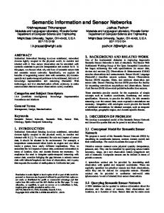
Figure 5.11: Multiratecast to four destinations d1 , d2 , d3 , and d4 . Numbers inside circles indicate the rate at which the corresponding node retransmits.
5.3.1
Rate-based metric
As discussed in [LCG+ 09], the hop count and retransmission number metrics do not reflect the real efficiency of a path in a multiple rate context, as the transmission rate can differ from one relay node to another. This idea is illustrated on Figure 5.3.1, where two different paths are proposed to serve a given set of destinations (with given rate requirements). Here the shorter path is the most expensive if we consider the number of messages to be effectively sent, that is the cumulative rate of retransmissions. Therefore, in order to measure this efficiency, the better choice is to use the sum of the (output) rates at each relay node, which is directly proportional to the number of messages to be sent. More formally, for a given set of relay nodes R = {r1 , r2 , ...r|R| } composing a P|R| multicast path, the overall path cost is defined as i=1 rate(ri ).
5.3.2
Geographical rate-based multicast
[LCG+ 09] proposed two localized geographical multiratecast protocols: Maximum Rate Multicast (MRM) and Optimal Rate Cost Multicast (ORCM). These two protocols are similar to PBM and GMR (described in Section 1 of this chapter) in the sense where they both extend the Greedy Face Greedy principle ([BMSU99], or Chapter 4 Section 5) to the multicast context, and take into account the wireless multicast advantage. The major difference is that they consider the different rates while making decisions, and aim at minimizing the rate-based metric described in the previous paragraph. Regarding assumptions, the protocols assume an ideal MAC layer without loss and that each node is individually capable of forwarding data at the maximum rate among destinations. The routing choices are solely made by looking at local neighbor positions with respect to destination positions, there is no routing table nor global overlay structure needed to be built. Finally, the network topology can change between two consecutive routing tasks without other cost than updating the new positions of destinations or the sources, if changed. Both protocols differ only on their greedy mode. The greedy mode is as
CHAPTER 5. XCASTING
19 d1 (40)
n1 d2 (10)
c
n2 d3 (30) n3
The highest rate destination, d1 , is assigned to the neighbor that provides the most advance toward it, n1 . Then all the destinations for which n1 provide any advance are assigned to it (d2 and d3 ). The process start anew with the remaining destinations, and d4 is assigned to n3 .
d4 (20)
Figure 5.12: Example scenario for MRM follows: at each hop, a set of next forwarding nodes is selected by the current node. Each of these nodes is given the responsibility of one or part of the destinations, and will repeat the same selection afterward, until the destinations are reached. The only difference between the two proposed protocols lies in their method to select the right neighbors at each hop. The first protocol, MRM, chooses them linearly by prioritizing the more demanding destinations, while the second, ORCM, evaluates different possible routing choices by combining distance progression and rate considerations, thereby implementing the more general concept of best cost over progress ratio ([KNS05], or Chapter 4 Section 3). Note that in order to apply such routing, message headers must include, in addition to their positions, the required rate of the destinations. Maximum Rate Multicast protocol (MRM) The basic idea behind MRM is to give priority to destinations that have the highest required rate. More precisely, at each hop, current node considers the destination that has the highest rate requirement, and determines what neighbor provides the most advance toward it. This neighbor is selected, and all the destinations for which it provides any progression are assigned to it. Then the process is repeated for the remaining destinations, until all of them are assigned. Finally, the message is sent. This process is illustrated on a simple scenario in Figure 5.12. Optimal Rate Cost Multicast protocol (ORCM) Following the example of PBM and GMR (both discussed Section 5.1.2 above), the idea behind ORCM is to evaluate different routing choices and then select the best ranked. In order to maintain a moderate calculation complexity, ORCM adapts its strategy to the number of destinations. If this number is under a given threshold, then it applies the same strategy as PBM by generating and evaluating all possible combinations (i.e., all possible arrangements of destination subsets, or partitioning, such that the destinations of each subset
CHAPTER 5. XCASTING
20
are assigned to a same neighbor). If the number of destinations is above the threshold, then it applies the strategy of GMR, which consists in computing an initial default partitioning (where destinations are grouped according to the most appropriate neighbor to serve them), and then to iterate a merge process to optimize it. The choice for the threshold value basically depends on the expected computational power of the nodes (a threshold of 6 was considered in [LCG+ 09]). d1 (r1 ) n1 d2 (r2 )
c d3 (r3 ) n2 d4 (r4 )
Figure 5.13: Example scenario for ORCM Let us consider the simple scenario given in Figure 5.13, where the current node c wants to select the next forwarding nodes toward d1 , d2 , d3 , and d4 (each having possibly a different rate requirement), and has the choice between using only n1 , only n2 , or both for different destinations. We illustrate here the two high-level strategies, depending on whether the number of destinations (4) is under, or above the threshold. Strategy 1: evaluation of all set partitions. There is 14 possible ways of partitioning the destinations: P1 P2 P3 P4 P5
= = = = =
{{d1 , d2 , d3 , d4 }} {{d1 }, {d2 , d3 , d4 }} {{d2 }, {d1 , d3 , d4 }} {{d3 }, {d1 , d2 , d4 }} {{d4 }, {d1 , d2 , d3 }}
P6 = {{d1 , d2 }, {d3 , d4 }} P7 = {{d1 , d3 }, {d2 , d4 }} P8 = {{d1 , d4 }, {d2 , d3 }} P9 = {{d1 }, {d2 }, {d3 , d4 }} P10 = {{d1 }, {d3 }, {d2 , d4 }}
P11 P12 P13 P14
= = = =
{{d2 }, {d3 }, {d1 , d4 }} {{d2 }, {d4 }, {d1 , d3 }} {{d3 }, {d4 }, {d1 , d2 }} {{d1 }, {d2 }, {d3 }, {d4 }}
Since there are only two neighbors considered here, the partitions from P9 to P14 do not make sense and can be discarded. ORCM will then evaluate every partitioning from P1 to P8 , and select the best ranked. Based on this best partitioning, each subset will be assigned to a given neighbor (the one minimizing the sum of remaining distances toward the corresponding destinations). Strategy 2: initial partitioning and merge process. As with GMR, an initial partitioning is generated, where each subset represents the destinations for which the best neighbor is the same, which leads to P 0 = {{d1 , d2 }, {d3 , d4 }}, where n1 serves {d1 , d2 } and n2 serves {d3 , d4 }. Then the merge process leads to P 00 = {{d1 , d2 , d3 , d4 }}, because it has a better evaluation that P 0 . All the destinations are then assigned to a same neighbor (the one minimizing the sum of remaining distances toward these destinations).
CHAPTER 5. XCASTING
21
For the evaluation of a given partitioning, ORCM implements, as GMR, the the concept of cost over progress ratio. However, here, the ratio formula is elaborated with the aim of minimizing the new rate-based metric. Three possible methods were proposed in [LCG+ 09] to calculate the cost over progress ratio of a given partitioning, but one of them always outperformed the two others, we thus limit the presentation to this one. In order to simplify the formula, the following notations can be introduced: - given a set of destinations D = {d1 , d2 , . . . , d|D| }, the notation rate(D) = max(rate(d) : d ∈ D), refers to the highest rate among these destinations. - given a current node c, one of its neighbors n, and a destination d, the notation progress(c, n, d) = dist(c, d) − dist(n, d), stands for the progression that n offers from c to d. - given a current node c, one of its neighbors n, and a set of destinations D = P|D| {d1 , d2 , . . . , d|D| }, the notation progress(c, n, D) = i=1 progress(c, n, di ), represents the cumulative progress that n offers from c toward these destinations. - finally, N (c) stands for the set of neighbors of a node c. The cost over progress ratio of a given partitioning P = {M1 , M2 , ..., M|P | }, where each Mi is one of the subsets, is defined as the sum of all subset rates, divided by the sum of all maximum subset distance progress. The intuitive idea behind this method is to choose, for each individual subset, the forwarding neighbor that will best profit the whole destination set: P|P | rate(Mi ) i=1 ratio(P ) = P|P | i=1
max(progress(c,n,Mi ):n∈N (c))
Note that if max(progress(c, n, Mi : n ∈ N (c)) is negative for any of the subsets, then the corresponding partitioning is discarded. In terms of the new rate-based metric, simulations showed a slight advantage for ORCM over MRM when a small number of destinations are considered (i.e., when ORCM evaluates all possible combinations), and a stronger advantage for MRM otherwise. MRM has also the advantage of a very lower computational cost, even when ORCM does not consider all the destination set partitions. Regarding the absolute efficiency of these protocols, simulations have been run to compare them with a sum of unicast, and shown an important overall cost advantage for them. Note that as the variance of rate distribution increases, the sum of unicast becomes more efficient than a non-rate-based multicast (which sends the message to all the nodes at the highest rate). An interesting question could be how these protocols behave comparatively to the optimal solution. Answering this question requires now to design good approximation algorithms for this NP-complete problem.
5.4
Anycasting with guaranteed delivery
In the anycasting problem, a source node wants to send a message to any node that belongs to a given set of destinations. In the context of IP networks, this
CHAPTER 5. XCASTING
22
problem was first formulated in the RFC 1546 as follows: “the host transmits a datagram to an anycast address and the Internetwork is responsible for providing best-effort delivery of the datagram to at least one, and preferably only one” (this was later reformulated in RFC 2373, in the context of IPv6). However, a number of articles refer to the anycasting problem while solving a different problem. For example, in [CDC+ 04] and [JK07], the term ’anycasting’ corresponds to the first stage of some geocasting protocols (see Section 2), which consists in reaching any node inside a given geographical region. In the present section, we consider that anycasting typically occurs when a sensor wants to report its data to an actuator, but does not care about which one of them will effectively receive the report. Such protocol should try to reach the actuator being the closest to the reported event in order to minimize the energy consumption induced by the report. Finally, actuators must be considered by the protocol as possibly scattered all over the network. While a number of anycasting protocols were designed for wired networks [WHH07], only a few have been designed for wireless networks, and most of them are adaptations of an anycast routing for wired networks [ABS03], which rely on flooding techniques. Among other anycasting protocols for wireless sensor networks, in [HBJ05], a shortest path anycast tree rooted at each source is constructed for each event source. Sinks are the only leaves of the tree and can dynamically join/leave the tree, which is updated accordingly. Data is delivered to the nearest sink on the tree. The algorithm thus simultaneously maintains paths to all sinks, and requires memorization of routing steps. Algorithms that rely on flooding turn very costly in large networks, and those relying on global structures, such as trees, are very costly to build and maintain as the network becomes larger or dynamic. For these reasons, localized and positionbased (geographic) protocols are preferred in the context of sensor and actuator networks, although they require that the positions of actuators are known by the sensor nodes. Let us introduce a few notations here. They will be used in the following paragraphs. Given two nodes u and v, we denote by |uv| the distance between them. Given a distance d, we denote by power(d) the amount of energy required to transfer a message over this distance. This power is roughly proportional to dα + c, where α represents the signal strength attenuation factor and c is a constant factor representing the minimal energy consumption induced by the transfer (see Chapter 1 for more details on energy models). Finally, given a sensor node s, we denote by A(s) the actuator that is the closest to s. The first position-based anycasting protocol was proposed in [MPA05]. This protocol attempts to minimize the energy consumption as follows. In the startup phase, each sensor node s selects one of its neighbor to act as its next hop toward an actuator. This selection is done by choosing the neighbor n that minimizes power(|sn|) + power(|nA(n)|). Despite the claim of the authors, this localized anycasting algorithm does not really optimize the power consumption because the neighbor selection is based on very long edges |nA(n)|, which are not power optimal. Further, the protocol does not guarantee the delivery in presence of void areas.
CHAPTER 5. XCASTING
23
In [MSS08], three localized and position-based protocols were proposed. These protocols are three different adaptations of the Greedy-Face-Greedy (GFG) principle to the context of anycasting, and consequently guarantee the delivery to the destination (i.e., to any actuator). The first protocol, GFGA, attempts to minimize the number of hops, while the second, COPA, and the third, EEGDA, focus on minimizing the energy consumption. The next paragraph briefly describes the three selection methods. 1. GFGA selects the neighbor n for which |nA(n)| is minimized (|sA(s)| − |nA(n)| is maximized), in other words it selects the neighbor that provides the highest advance toward any actuator. Note that in this formula A(s) and A(n) can be different, which reflects the key concept of anycasting. 2. COPA relies on the cost over progress ratio ([KNS05], or Chapter 4 Section 3), where cost is the estimated energy consumption for the next hop, and progress is the distance progression toward any actuator. More prepower(|sn|) is chosen cisely, for a sensor s, the neighbor n minimizing |sA(s)|−|nA(n)| (two more sophisticated variants are also proposed, but have very similar performance). 3. EEGA is an enhancement of COPA that is inspired from the protocol EtE [EMS08]. The solution is more energy-efficient than COPA but has a higher computing complexity. The idea behind it is that once a neighbor n is selected as next hop (according to any energy-related cost formula), it may be sometimes more energy-efficient to use one or several additional neighbors to reach n (especially if the signal strength attenuation factor α is high). This is done by calculating the Energy-weighted Shortest Path (ESP) from the current node to each neighbor (which can be done locally since nodes are aware of the positions of their neighbors), and then forwarding the message to the first node on the ESP to n. Regarding the anycasting aspects, the essence of all these solutions is that the destination can be changed during the routing process, to select another actuator if desirable. Such scenario is illustrated on Figure 5.14, where a sensor node S wants to initiate a report. According to the relative distances of actuators, S selects A1 as destination, and starts greedy advance toward it. Once at B, there is no neighbor closer to any actuator than B to A1 . The protocol thus switches to recovery mode (here a right-hand face traversal is started). If the unicast version of GFG were used here, the recovery mode would continue until reaching node D, from which greedy advance would be resumed toward A1 . Here however, node C notices that actuator A2 is closer to itself than A1 was to B. A2 is thus chosen as the new destination, and greedy mode is resumed toward it. Finally, upon receiving the message, node E performs a last modification without breaking the greedy procedure, by switching the destination to A3 , now closer than A2 .
CHAPTER 5. XCASTING
24
A2
A1 D C
A3 E
B
S
Figure 5.14: Geographic anycasting based on an adaptation of GFG.
Bibliography [ABS03] B. Awerbuch, A. Brinkmann, and C. Scheideler. Anycasting and multicasting in adversarial systems: Routing and admission control. In 30th International Colloquium on Automata, Languages, and Programming (ICALP’03), Eindhoven, Netherlands., 2003. [BFC93] T. Ballardie, P. Francis, and J. Crowcroft. Core based trees (cbt). SIGCOMM Comput. Commun. Rev., 23(4):85–95, 1993. [BMSU99] P. Bose, P. Morin, I. Stojmenovic, and J. Urrutia. Routing with guaranteed delivery in ad hoc wireless networks. In 3rd international workshop on discrete algorithms and methods for mobile computing and communications (DIALM ’99), pages 48–55, New York, NY, USA, 1999. [BMSU01] P. Bose, P. Morin, I. Stojmenovic, and J. Urrutia. Routing with guaranteed delivery in ad hoc wireless networks. Wirel. Netw., 7(6):609–616, 2001. [CDC+ 04] S. Chen, C. Dow, S. Chen, J. Lin, and S. Hwang. An efficient anycasting scheme in ad-hoc wireless networks. In Consumer Communications and Networking Conference, pages 178–183, Las Vegas, Nevada, USA, 2004. [DC90] S.E. Deering and D.R. Cheriton. Multicast routing in datagram internetworks and extended lans. ACM Trans. Comput. Syst., 8(2):85–110, 1990. [DEF+ 94] S. Deering, D. Estrin, D. Farinacci, V. Jacobson, C.G. Liu, and L. Wei. An architecture for wide-area multicast routing. SIGCOMM Comput. Commun. Rev., 24(4):126–135, 1994. [DPH08] S. Das, H. Pucha, and Y.C. Hu. Distributed hashing for scalable multicast in wireless ad hoc networks. IEEE Trans. Parallel Distrib. Syst., 19(3):347–362, 2008. [DSW02] S. Datta, I. Stojmenovic, and J. Wu. Internal node and shortcut based routing with guaranteed delivery in wireless networks. Cluster Computing, 5(2):169–178, April 2002. 25
BIBLIOGRAPHY
26
[EMS08] E.H. Elhafsi, N. Mitton, and D. Simplot-Ryl. Energy efficient geographic path discovery with guaranteed delivery in ad hoc and sensor networks. In IEEE PIMRC, Cannes, France, 2008. [GLAM99] J. Garcia-Luna-Aceves and E. Madruga. The core-assisted mesh protocol. IEEE Journal on Selected Areas in Communications, 17:1380–1394, 1999. [HBJ05] W. Hu, N. Bulusu, and S. Jha. A communication paradigm for hybrid sensor/actuator networks. Journal of Wireless Information Networks, 12(1):47–59, 2005. [JC98] L. Ji and M.S. Corson. A lightweight adaptive multicast algorithm. Global Telecommunications Conference, 1998. GLOBECOM 98. The Bridge to Global Integration. IEEE, 2:1036–1042 vol.2, 1998. [JC01] L. Ji and M.S. Corson. Differential destination multicast-a manet multicast routing protocol for small groups. INFOCOM 2001. Twentieth Annual Joint Conference of the IEEE Computer and Communications Societies. Proceedings. IEEE, 2:1192–1201 vol.2, 2001. [JJ01] J.G. Jetcheva and D.B. Johnson. Adaptive demand-driven multicast routing in multi-hop wireless ad hoc networks. In MobiHoc ’01: Proceedings of the 2nd ACM international symposium on Mobile ad hoc networking & computing, pages 33–44, New York, USA, 2001. ACM. [JK07] P. Jeon and G. Kesidis. Geoppra: An energy efficient geocasting protocol in mobile ad hoc networks. In Intl. Conf. on Networking (ICN), 2007. [JS02] C. Jaikaeo and C.-C. Shen. Adaptive backbone-based multicast for ad hoc networks. Communications, 2002. ICC 2002. IEEE International Conference on, 5:3149–3155 vol.5, 2002. [Kar72] R. M. Karp. Reducibility among combinatorial problems. In R. E. Miller and J. W. Thatcher, editors, Complexity of Computer Computations, pages 85–103. Plenum Press, 1972. [KAS08] F.A. Khan, K.-J. Ahn, and W.-C. Song. Geocasting in wireless ad hoc networks with guaranteed delivery. pages 213–222, 2008. [KDHS08] D. Koutsonikolas, S.M. Das, Y.C. Hu, and I. Stojmenovic. Hierarchical geographic multicast routing for wireless sensor networks. Wireless Networks, October 2008.
BIBLIOGRAPHY
27
[KNS05] J. Kuruvila, A. Nayak, and I. Stojmenovic. Hop count optimal position-based packet routing algorithms for ad hoc wireless networks with a realistic physical layer. Selected Areas in Communications, IEEE Journal on, 23(6):1267–1275, June 2005. [LCG+ 09] X. Liu, A. Casteigts, N. Goel, A. Nayak, and I. Stojmenovic. Multiratecast in wireless fault-tolerant sensor and actuator networks. Manuscript, 2009. [LGC99] S.-J. Lee, M. Gerla, and C.-C. Chiang. On-demand multicast routing protocol. Wireless Communications and Networking Conference, 1999. WCNC. 1999 IEEE, pages 1298–1302 vol.3, 1999. [MFWL03] M. Mauve, H. F¨ ußler, J. Widmer, and T. Lang. Position-based multicast routing for mobile ad-hoc networks. SIGMOBILE Mob. Comput. Commun. Rev., 7(3):53–55, 2003. [Moy94] J. Moy. Multicast routing extensions for ospf. Commun. ACM, 37(8):61–ff., 1994. [MPA05] T. Melodia, V.C. Pompili, and I. Akyildiz. A distributed coordination framework for wireless sensor and actor networks. In ACM Mobihoc, pages 99–110, 2005. [MSS08] N. Mitton, D. Simplot-Ryl, and I. Stojmenovic. Guaranteed delivery for geographical anycasting in wireless multi-sink sensor and sensoractor networks. 2008. [MYT04] A. Mizumoto, H. Yamaguchi, and K. Taniguchi. Cost-conscious geographic multicast on manet. Sensor and Ad Hoc Communications and Networks, 2004. IEEE SECON 2004. 2004 First Annual IEEE Communications Society Conference on, pages 44–53, Oct. 2004. [NAX06] U.T. Nguyen, A. Asif, and X. Xiong. Multirate-aware multicast routing in manets. Mobile Adhoc and Sensor Systems (MASS), 2006 IEEE International Conference on, pages 554–557, Oct. 2006. [Nic04] D. Niculescu. Positioning in ad hoc sensor networks. Network, IEEE, 18(4):24–29, July-Aug. 2004. [RGS05] P.M. Ruiz and A.F. Gomez-Skarmeta. Approximating optimal multicast trees in wireless multihop networks. Computers and Communications, IEEE Symposium on, 0:686–691, 2005. [RP00] E. Royer and C. Perkins. Multicast ad hoc on-demand distance vector (maodv) routing, 2000. [RS07] P.M. Ruiz and I. Stojmenovic. Handbook on Approximation Algorithms and Metaheuristics, chapter Cost-efficient multicast routing in ad hoc and sensor networks, pages 1–14. Number 65. Chapman & Hall/CRC (Teofilo Gonzalez, ed.), 2007.
BIBLIOGRAPHY
28
[SH04] K. Seada and A. Helmy. Efficient geocasting with perfect delivery in wireless networks. Wireless Communications and Networking Conference, 2004. WCNC. 2004 IEEE, 4:2551–2556 Vol.4, March 2004. [SPD04] G. Singh, S. Pujar, and S. Das. Rate-based data propagation in sensor networks. Wireless Communications and Networking Conference, 2004. WCNC. 2004 IEEE, 4:2480–2485 Vol.4, March 2004. [SRL99] I. Stojmenovic, A.P. Ruhil, and D.K. Lobiyal. Voronoi diagram and convex hull based geocasting and routing in wireless networks. Technical report, SITE, University of Ottawa, Dec 1999. [SRLS07] J.A. Sanchez, P.M. Ruiz, X. Liu, and I. Stojmenovic. Bandwidthefficient geographic multicast routing protocol for wireless sensor networks. Sensors Journal, IEEE, 7(5):627–636, May 2007. [SSB99] P. Sinha, R. Sivakumar, and V. Bharghavan. Mcedar: multicast core-extraction distributed ad hoc routing. Wireless Communications and Networking Conference, 1999. WCNC. 1999 IEEE, pages 1313–1317 vol.3, 1999. [Sto04] I. Stojmenovic. Geocasting with guaranteed delivery in sensor networks. Wireless Communications, IEEE, 11(6):29–37, Dec. 2004. [Sto06] I. Stojmenovic. Geocasting in ad hoc and sensor networks. In In Theoretical and Algorithmic Aspects of Sensor, Ad Hoc Wireless and Peer-to-Peer Networks (Jie Wu, ed., pages 79–97. Auerbach Publications (Taylor & Francis Group), 2006. [WC06] S. Wu and K.S. Candan. GMP: Distributed geographic multicast routing in wireless sensor networks. Distributed Computing Systems, International Conference on, 0:49, 2006. [WHH07] C.-J. Wu, R.-H. Hwang, and J.-M. Ho. A scalable overlay framework for internet anycasting service. In Symposium on Applied Computing (SAC), pages 193–197, New York, USA, 2007. [WT99] C.W. Wu and Y.C. Tay. Amris: a multicast protocol for ad hoc wireless networks. Military Communications Conference Proceedings, 1999. MILCOM 1999. IEEE, 1:25–29 vol.1, 1999. [XTML02] J. Xie, R.R. Talpade, A. Mcauley, and M. Liu. AMRoute: ad hoc multicast routing protocol. Mob. Netw. Appl., 7(6):429–439, 2002.