Multicollinearity in Regression Models

© 2002 Jeeshim and KUCC625. (2003-05-09)

Multicollinearity.doc

Multicollinearity in Regression Models Introduction Multicollinearity is a high degree of correlation (linear dependency) among several independent variables. It commonly occurs when a large number of independent variables are incorporated in a regression model. It is because some of them may measure the same concepts or phenomena. Only existence of multicollinearity is not a violation of the OLS assumption. However, a perfect multicollinearity violates the assumption that X matrix is full ranked, making OLS impossible. When a model is not full ranked, that is, the inverse of X cannot be defined, there can be an infinite number of least squares solutions. Symptoms of mulitcollinearity may be observed in situations: (1) small changes in the data produce wide swings in the parameter estimates; (2) coefficients may have very high standard errors and low significance levels even though they are jointly significant and the R 2 for the regression is quite high; (3) coefficients may have the “wrong” sign or implausible magnitude (Greene 2000: 256). Multicollnearity has following consequences. 1. Variance (SEE) of the model and variances of coefficients are inflated. As a result, any inference is not reliable and the confidence interval becomes wide. 2. Estimates remain BLUE, so does R 2 3. Ryx2 1 ... x k < ryx2 1 + ryx2 2 + ... + ryx2 k . Detecting Multicollinearity There is no clear-cut criterion for evaluating multicollinearity of linear regression models. We may compute correlation coefficients of independent variables. But high correlation coefficients do not necessarily imply multicollinearity. We can make a judgment by checking related statistics, such as tolerance value or variance inflation factor (VIF), Eigenvalue, and condition number. In the SAS REG procedure, TO L, VIF, COLLIN options of the MODEL statement produces such statistics. Note that the COLLIN option is for eigenvalues and condition numbers. SAS follows Belsley, Kuh, and Welsch (1980) approach. 1. Tolerance value and VIF: 1 − Rk2 and 1 (1 − Rk2 ) The ith tolerance value is defined as 1 − Rk2 , Rk2 is the coefficient of determination for regression of the ith independent variable on all the other independent variables: X k = X others . In the following example, the tolerance value of INCOME .0612 is calculated as1-.9388, where .9388 is 2 Rincome . Variance inflation factor (VIF) is just the reciprocal of a tolerance value, thus low tolerances correspond to high VIF. VIF 16.33392 of INCOME is just 1/.0612. VIF shows how multicollinearity has increased the instability of the coefficient estimates (Freund and Littell 2000: 98). Put differently, it tells you how "inflated" the variance of the coefficient is, compared to what it would be if the variable

http://php.indiana.edu/~kucc625

1

© 2002 Jeeshim and KUCC625. (2003-05-09)


were uncorrelated with any other variable in the model (Allison 1999: 48-50). PROC REG; MODEL expend = age rent income inc_sq /TOL VIF COLLIN; RUN; The REG Procedure Model: MODEL1 Dependent Variable: expend Analysis of Variance

Source

DF

Sum of Squares

Mean Square

Model Error Corrected Total

4 67 71

1749357 5432562 7181919

437339 81083

Root MSE Dependent Mean Coeff Var

284.75080 262.53208 108.46324

R-Square Adj R-Sq

F Value

Pr > F

5.39

0.0008

0.2436 0.1984

Parameter Estimates

Variable

DF

Parameter Estimate

Standard Error

t Value

Pr > |t|

Tolerance

Variance Inflation

Intercept age rent income inc_sq

1 1 1 1 1

-237.14651 -3.08181 27.94091 234.34703 -14.99684

199.35166 5.51472 82.92232 80.36595 7.46934

-1.19 -0.56 0.34 2.92 -2.01

0.2384 0.5781 0.7372 0.0048 0.0487

. 0.73398 0.69878 0.06122 0.06575

0 1.36243 1.43106 16.33392 15.21011

Collinearity Diagnostics

Number

Eigenvalue

Condition Index

1 2 3 4 5

4.08618 0.50617 0.37773 0.02190 0.00801

1.00000 2.84125 3.28903 13.66046 22.57958

Collinearity Diagnostics

Number 1 2 3 4 5

------------------------Proportion of Variation-----------------------Intercept age rent income inc_sq 0.00144 0.01512 0.00084302 0.47504 0.50755


0.00193 0.01185 0.00213 0.96708 0.01701

0.01672 0.29511 0.57397 0.09462 0.01957

0.00068914 7.577405E-7 0.00220 0.01820 0.97891

0.00170 0.01689 0.04095 0.01121 0.92924

2

© 2002 Jeeshim and KUCC625. (2003-05-09)


However, there is no formal criterion for determining the bottom line of the tolerance value or VIF. Some argue that a tolerance value less than .1 or VIF greater than 10 roughly indicates significant multicollinearity. Others insist that magnitude of model’s R 2 be considered determining significance of multicollinearity. Klein (1962) suggests alternative criterion that Rk2 exceeds R 2 of the regression model. In this vein, if VIF is greater than 1 /(1 − R 2 ) or a tolerance value is less than (1 − R 2 ) , multicollinearity can be considered as statistically significant. . regress expend age rent income inc_sq if expend~=0 Source | SS df MS -------------+-----------------------------Model | 1749357.01 4 437339.252 Residual | 5432562.03 67 81083.0153 -------------+-----------------------------Total | 7181919.03 71 101153.789

Number of obs F( 4, 67) Prob > F R-squared Adj R-squared Root MSE

= = = = = =

72 5.39 0.0008 0.2436 0.1984 284.75

-----------------------------------------------------------------------------expend | Coef. Std. Err. t P>|t| [95% Conf. Interval] -------------+---------------------------------------------------------------age | -3.081814 5.514717 -0.56 0.578 -14.08923 7.925606 rent | 27.94091 82.92232 0.34 0.737 -137.5727 193.4546 income | 234.347 80.36595 2.92 0.005 73.93593 394.7581 inc_sq | -14.99684 7.469337 -2.01 0.049 -29.9057 -.0879859 _cons | -237.1465 199.3517 -1.19 0.238 -635.0541 160.7611 ------------------------------------------------------------------------------

. vif Variable | VIF 1/VIF -------------+---------------------income | 16.33 0.061222 inc_sq | 15.21 0.065746 rent | 1.43 0.698784 age | 1.36 0.733980 -------------+---------------------Mean VIF | 8.58

In the above example, INCOME and INC_SQ are suspected of causing multicollnearity since their tolerance values are less than .1 or VIFs are greater than 10. Note that the 1/VIF is nothing but the tolerance value. 2. Engenvalues (characteristic roots) and condition numbers (or condition ind ices) In Ac − λc (c’c=1 for normalization), ? and c are respectively called characteristic root and characteristic vector of the square matrix A. A = CΛC' = ∑ λk c k c 'k A is written as the eigenvalue (or “own” value) decomposition of A, the sum of K rank one matrices. They are computed by a multivariate statistical technique called the principal component


3

© 2002 Jeeshim and KUCC625. (2003-05-09)


analysis. Z = XΓ , where Z is the matrix of principal component variables and Γ is the matrix of coefficients that relate Z to X (the matrix of observed variables). Principal components are obtained by computing the eigenvalues and eigenvectors of the correlation or covariance matrix. The eigenvalues (or characteristic roots) are the variances of the components. If the correlation matrix has been used, the variance of each input variable is one; the sum of variances (eigenvalues) of the component variables is equal to the number of variables (Freund and Littell 2000: 99). Eigenve ctors, the columns of Γ , are the coefficients of the linear equations that relate the component variables (latent variables or factors) to the original variables (manifest variables). A set of eigenvalues of relatively equal magnitudes indicates that there is little multicollinearity (Freund and Littell 2000: 99). A small number of large eigenvalues indicates that a small number of component variables describe most of the variability of the original observed variables (X). Because of the scale constraint, a number of large eigenvalues implies that there will be some small eigenvalues or some small variances of component variables (Z). A zero eigenvalue means perfect collinearity among independent variables and very small eigenvalues implies severe multicollinearity. The COLLIN option computes eigenvalues and eigenvectors of the scaled X’X with 1s on the diagonal, while the COLLINOINT uses X’X without 1’s column as a correlation matrix. Condition numbers or condition indices are square roots of the ratios of the largest eigenvalues to individual ith eigenvalues. Eigenvalues are just characteristic roots of X’X. Conventionally, an eigenvalue close to zero (say less than .01) or condition number greater than 50 (30 for conservative persons) indicates significan multicollinearity. Belsley, Kuh, and Welsch (1980) insist 10 to 100 as a beginning and serious points that collinearity affects estimates. The SAS COLLIN option produces eigenvalues and condition index, as well as proportions of variances with respect to each independent variable. The proportion tells how much (percentage) of the variance of the parameter estimate (coefficient) is associated with each eigenvalue. A high proportion of variance of an independent variable coefficient reveals a strong association with the eigenvalue. Thus, if an eigenvalue is small enough and some independent variables show high proportions of variation with respect to the eigenvalue, we may conclude that these independent variables have significant linear-dependency (correlation). In the above SAS output, eigenvalues of INCOME and INC_SQ are respectively .0219 and .0080. The corresponding condition indices are 13.6605 and 22.5796. So they are marginally significant. Let us look at the proportions of variance for INCOM and INC_SQ that has small eigenvalues. AGE has a high proportion (.9671) with respect to INCOME, which shows another high proportion (.9789) against INC_SQ. Considering all indicators together, we can conclude INC_SQ is linearly dependent on INCOME, causing multicollinearity in the regression model. Statistics Tolerance Value VIF Eigenvalue Condition Index Proportion of Varia tion 2 Greater than Critical Less than (1 − R ) Greater than 50 Less than .01 Greater than .8 (or .7) 2 (or 30) 1/ (1 − R ) Value Roughly less than .1 Method Rk2 fro m a regression X k = X others Principal Component Analysis on the X’X matrix


4

© 2002 Jeeshim and KUCC625. (2003-05-09)


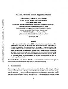
Let us confirm the conclusion by drawing plots and computing correlation coefficients. Correlation coefficients indicate all independent variables are significantly related to each other. Note that the magnitude of INCOME and INC_SQ is pretty high (.9626). Look at the plots. The left plot illustrates that despite large variation, income tends to increase as people get old. Obviously, income is highly correlated with income squared (INC_SQ). So it is reasonable to conclude that INC_SQ causes multicollinearity in the model. . pwcorr age rent income inc_sq, sig star(.05) | age rent income inc_sq -------------+-----------------------------------age | 1.0000 | rent | 0.2865* 1.0000 | 0.0039 | income | 0.2685* 0.3483* 1.0000 | 0.0069 0.0004 | inc_sq | 0.2187* 0.3202* 0.9626* 1.0000 | 0.0288 0.0012 0.0000

. graph age income . graph inc_sq income 100

age

inc_sq

55

20

2.25 1.5

10 income

1.5

10 income

Troubleshooting 1. Change specification by omitting or adding independent variables. We may consider quadratic and other polynomial forms of independent variables. However, omitting correlated (but relevant) independent variables causes coefficients biased, their variance smaller, and SSE, s 2 , biased. Including irrelevant correlated variables causes coefficients and s 2 unbiased. But it cause overfitting the model. If the variable is highly correlated to some of existing independent variables, the variances of estimates become inflated (Greene 2000: 334-338). But just relying upon variable selection methods may result in data dredging, data fishing, or data technique trap.


5

© 2002 Jeeshim and KUCC625. (2003-05-09)


Let us omit the INC_SQ and run the regression. Note the R 2 became lower and root MSE increased. J test results in a small F score .001, which indicates that omission is not appropriate though. . regress expend age rent income if expend~=0 Source | SS df MS -------------+-----------------------------Model | 1422494.15 3 474164.716 Residual | 5759424.89 68 84697.4248 -------------+-----------------------------Total | 7181919.03 71 101153.789

Number of obs F( 3, 68) Prob > F R-squared Adj R-squared Root MSE

= = = = = =

72 5.60 0.0017 0.1981 0.1627 291.03

-----------------------------------------------------------------------------expend | Coef. Std. Err. t P>|t| [95% Conf. Interval] -------------+---------------------------------------------------------------age | -.7769176 5.512819 -0.14 0.888 -11.77758 10.22374 rent | 32.08765 84.72408 0.38 0.706 -136.9766 201.1519 income | 79.83579 23.67235 3.37 0.001 32.59835 127.0732 _cons | .3972042 163.9851 0.00 0.998 -326.83 327.6244 ------------------------------------------------------------------------------

. vif Variable | VIF 1/VIF -------------+---------------------rent | 1.43 0.699218 income | 1.36 0.737074 age | 1.30 0.767227 -------------+---------------------Mean VIF | 1.36

SAS produces eigenvalue, condition index, and corresponding proportion of variance. Although AGE and INCOME shows high proportion of variance, any of tolerance value (or VIF), eigenvalue, and condition index indicates serious multicollinearity. . Collinearity Diagnostics

Number

Eigenvalue

Condition Index

1 2 3 4

3.41087 0.46276 0.10497 0.02140

1.00000 2.71491 5.70031 12.62492

--------------Proportion of Variation------------Intercept age rent income 0.00342 0.01385 0.05569 0.92704

0.00306 0.00558 0.04076 0.95060

0.02393 0.73391 0.12669 0.11548

0.01133 0.00238 0.98510 0.00119

2. Obtain more data (observations ) if problems arise because of a shortage of information. 3. Transform independent variables (take difference, logarithmic, or exponential) 4. Try biased estimation methods such as the ridge regression estimation (Judge et al. 1985) and incomplete principal component regression (Gurmu, Rilstone, and Stern 1999). The Ridge regression


6

© 2002 Jeeshim and KUCC625. (2003-05-09)


estimator, br = ( X ' X + rD ) −1 X ' y , has a covariance matrix unambiguously smaller than that of OLS. Incomplete principal component regression deletes from the principal component regression one or more of the transformed variables having small variances and then convert the resulting regression to the original variables (Freund and Littell 2000: 120). SAS REG procedure provides MODEL options for the two methods. PROC REG; MODEL depend = x1-x7 /PCOMIT= 1- 5; RUN; PROC REG; MODEL depend = x1-x7 /RIDGE=0 TO .5 BY .1; RUN;

Variable Selection SAS has the SELECTION option in the MODEL statement of the REG procedure to sort out plausible independent variables. The methods available are RSQUARE (R-Square selection), ADJRSQ (adjusted R-Square selection) BACKWARD (Backward elimination), FORWARD (Forward selection), STEPWISE (Stepwise selection), MAXR (Maximum R-Square improvement), and MINR (MinimumR-Square improvement). However, using the SELECTION option without know what is going on the model is not recommendable. PROC REG; MODEL expend = age rent income inc_sq /SELECTION=BACKWARD; RUN; Backward Elimination: Step 2 Variable age Removed: R-Square = 0.2397 and C(p) = 1.3433 Analysis of Variance

Source

DF

Sum of Squares

Mean Square

Model Error Corrected Total

2 69 71

1721522 5460396 7181919

860761 79136

F Value

Pr > F

10.88

F

Intercept income inc_sq

-304.14861 225.65551 -14.24923

160.70962 74.60287 7.18529

283441 724029 311221

3.58 9.15 3.93

0.0626 0.0035 0.0513

Bounds on condition number: 14.422, 57.686 -----------------------------------------------------------------------------------------All variables left in the model are significant at the 0.1000 level.

The above is a part of SAS output, which shows the last stage. The BACKWARD method chooses the combination of INCOME and INC_SQ, ignoring AGE and RENT.


7

© 2002 Jeeshim and KUCC625. (2003-05-09)


REFERENCES Belsley, David. A., Edwin. Kuh, and Roy. E. Welsch. 1980. Regression Diagnostics: Identifying Influential Data and Sources of Collinearity. New York: John Wiley and Sons. Freund, Rudolf J. and Ramon C. Littell. 2000. SAS System for Regression (Third edition). Cary, NC: SAS Institute. Greene, William H. 2000. Econometric Analysis (Fourth edition). Upper Saddle River, NJ: PrenticeHall. Gurmu, S., P. Rilstone, and S. Stern. 1999. “Semiparametric Estimation of Count Regression Models.” Journal of Econometrics, 88:1. 123-150.


8