order for the leading ones trailing zeros (LOTZ) problem. The first ...... convex and all constraint functions are locally concave, and the Fritz John conditions hold ...
Multicriteria Optimization and Decision Making Principles, Algorithms and Case Studies Michael Emmerich and Andr´e Deutz LIACS Master Course: Autumn/Winter 2006
2
Contents 1 Introduction 1.1 Viewing MOO as a task in system design 1.2 Formal Problem Definitions . . . . . . . 1.3 Pareto domination and incomparability . 1.4 Formal Definition of Pareto Dominance .
and analysis . . . . . . . . . . . . . . . . . . . . . . . . .
. . . .
. . . .
. . . .
4 . 6 . 8 . 11 . 12
2 Theoretical aspects of ordered sets 2.1 Axiomatic Definition of Orders . . 2.2 Preorders . . . . . . . . . . . . . . 2.3 Partial orders . . . . . . . . . . . . 2.4 Linear orders and anti-chains . . . 2.5 Hasse diagrams . . . . . . . . . . . 2.6 Comparing ordered sets . . . . . . 2.7 Representing orders as cones . . . .
. . . . . . .
. . . . . . .
. . . . . . .
. . . . . . .
. . . . . . .
. . . . . . .
. . . . . . .
. . . . . . .
. . . . . . .
. . . . . . .
. . . . . . .
. . . . . . .
. . . . . . .
15 15 16 18 19 19 20 23
3 Pareto optima and efficient points 3.1 Search Space vs. Objective Space . . . . 3.2 Global Pareto Fronts and Efficient Sets . 3.3 Weak efficiency . . . . . . . . . . . . . . 3.4 Characteristics of Pareto Sets . . . . . . 3.5 Optimality conditions based on level sets 3.6 Local Pareto Optimality . . . . . . . . . 3.7 Barrier Structures . . . . . . . . . . . . . 3.8 Shapes of Pareto Fronts . . . . . . . . .
. . . . . . . .
. . . . . . . .
. . . . . . . .
. . . . . . . .
. . . . . . . .
. . . . . . . .
. . . . . . . .
. . . . . . . .
. . . . . . . .
. . . . . . . .
. . . . . . . .
. . . . . . . .
27 27 29 30 31 32 35 38 41
. . . . . . .
. . . . . . .
4 Optimality conditions for differentiable problems 46 4.1 Linear approximations . . . . . . . . . . . . . . . . . . . . . . 46 4.2 Unconstrained Optimization . . . . . . . . . . . . . . . . . . . 47 1
4.3 Equality Constraints . . . . . . . . . . . . . . . . . . . . . . . 48 4.4 Inequality Constraints . . . . . . . . . . . . . . . . . . . . . . 53 4.5 Multiple Objectives . . . . . . . . . . . . . . . . . . . . . . . . 55 5 Scalarization Methods 5.1 Linear Aggregation . . . . . . . . . . . 5.2 Nonlinear Aggregation . . . . . . . . . 5.3 Multi-Attribute Utility Theory . . . . . 5.4 Distance to a Reference Point Methods
. . . .
. . . .
. . . .
. . . .
. . . .
. . . .
. . . .
. . . .
. . . .
. . . .
. . . .
. . . .
. . . .
57 58 60 61 67
6 Transforming Multicriteria into Constrained Single-Criterion Problems 71 6.1 Compromise Programming or ǫ-Constraint Methods . . . . . . 71 6.2 Concluding remarks on single point methods . . . . . . . . . . 75
I
Algorithms for Pareto Optimization
77
7 Pareto Front Computing with Deterministic Methods 78 7.1 Continuation methods . . . . . . . . . . . . . . . . . . . . . . 78
2
Preface Real world decision and optimization problems usually involve conflicting criteria. Ideal solutions are rather the exception than the rule. In this course we will deal with algorithmic methods for solving multi-objective optimization and decision making problems. The rich mathematical structure of such problems as well as their high relevance in various application fields led recently to a significant increase of research activities. In particular algorithms that make use of fast, parallel computing technologies are envisaged for tackling hard combinatorial and/or nonlinear application problems. In the course we will discuss the theoretical foundations of multi-objective optimization problems and their solution methods, including order and decision theory, analytical, interactive and meta-heuristic solution methods as well as state-of-the-art tools for their performance-assessment. Also an overview on decision aid tools and formal ways to reason about conflicts will be provided. All theoretical concepts will be accompanied by illustrative hand calculations and graphical visualizations during the course. In the second part of the course, the discussed approaches will be exemplified by the presentation of case studies from the literature, including various application domains of decision making, e.g. economy, engineering, medicine or social science. This reader is covering the topic of Multicriteria Optimization and Decision Making. Our aim is to give a broad introduction to the field, rather than to specialize on certain types of algorithms and applications. Exact algorithms for solving optimization algorithms are discussed as well as selected techniques from the field of metaheuristic optimization, which received growing popularity in recent years. The book provides a detailed introduction into the foundations and a starting point into the methods and applications for this exciting field of interdisciplinary science. Besides orienting the reader about state-of-the-art techniques and terminology, references are given that invite the reader to further reading and point to specialized topics. 3
Chapter 1 Introduction Multicriteria optimization and decision making is an exiting field of science. Part of its fascination stems from the fact that in MCO and MCDM different scientific fields are addressed. Firstly, to develop the general foundations and methods of the field one has to deal with structural sciences, such as algorithmics, relational logic, operations research, and numerical analysis: • How can we state a decision/optimization problem in a formal way? • What are the essential differences between single objective and multiobjective optimization? • How can we rank solutions? What different types of orderings are used in decision theory and how are they related to each other? • Given a decision model or optimization problem, which formal conditions need to be satisfied for solutions to be optimal? • How can we construct algorithms that obtain optimal solutions, or approximations to them, in an efficient way? • What is the geometrical structure of solution sets for problems with more than one optimal solution? Whenever it comes to decision making in the real world, these decisions will be made by people responsible for it. In order to understand how people come to decisions and how the psychology of individuals (cognition, individual decision making) and organizations (group decision making) needs to be studied. Questions like the following may arise: 4
• What are our goals? What makes it difficult to state goals? How do people define goals? Can the process of identifying goals be supported? • Which different strategies are used by people to come to decisions? How can satisfaction be measured? What strategies are promising in obtaining satisfactory decisions? • What are the cognitive aspects in decision making? How can decision support systems be build in a way that takes care of cognitive capabilities and limits of humans? • How do groups of people come to decisions? What are conflicts and how can they be avoided? How to deal with minority interests in a democratic decision process? Can these aspects be integrated into formal decision models? Moreover, decisions are always related to some real world problem. Given an application field, we may find very specific answers to the following questions: • What is the set of alternatives? • By which means can we retrieve the values for the criteria (experiments, surveys, function evaluations)? Are there any particular problems with these measurements (dangers, costs), and how to deal with them? What are the uncertainties in these measurements? • What are the problem-specific objectives and constraints? • What are typical decision processes in the field, and what implications do they have for the design of decision support systems? • Are there existing problem-specific procedures for decision support and optimization, and what about the acceptance and performance of these procedures in practice? In summary, this list of questions gives some kind of bird eye’s view of the field. However, in this book we will mainly focus on the structural aspects of multi-objective optimization and decision making. On the other hand, we also devote one chapter to people-centric aspects of decision making and one chapter to the problem of selecting, adapting, and evaluating MOO tools for application problems. 5
1.1
Viewing MOO as a task in system design and analysis
The discussion above can be seen as a rough sketch of questions that define the scope of multicriteria optimization and decision making. However, it needs to be clarified more precisely what is going to be the focus of this book. For this reason we want to approach the problem class from the point of view of system design and analysis. Here, with system analysis, we denote the interdisciplinary research field, that deals with the modeling, simulation, and synthesis of complex systems. Beside experimentation with a physical system, often a system model is used. Nowadays, system models are typically implemented as computer programs that solve (differential) equation systems, simulate interacting automata, or stochastic models. We will also refer to them as simulation models. An example for a simulation model based on differential equations would be the simulation of the fluid flow around an airfoil based on the Navier Stokes equations. An example for a stochastic system model, could be the simulation of a system of elevators, based on some agent based stochastic model. ! !
! ?
!
!
!
! !
? !
?
!
?
!
? ?
!
! !
?
Modelling Identification Calibration
Simulation Prediction Exploration
Optimization Inverse Design Control* *) if system (model) is dynamic
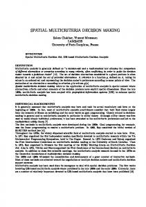
Figure 1.1: Different tasks in systems analysis.
6
In Figure 1.1 different tasks of systems analysis based on simulation models are displayed in a schematic way. Modeling means to identify the internal structure of the simulation model. This is done by looking at the relationship between known inputs and outputs of the system. In many cases, the internal structure of the system is already known up to a certain granularity and only some parameters need to be identified. In this case we usually speak of calibration of the simulation model instead of modeling. In control theory, also the term identification is common. Once a simulation-model of a system is given, we can simulate the system, i.e. predict the state of the output variables for different input vectors. Simulation can be used for predicting the output for not yet measured input vectors. Usually such model-based predictions are much cheaper than to do the experiment in the real world. Consider for example crash test simulations or the simulation of wind channels. In many cases, such as for future predictions, where time is the input variable, it is even impossible to do the experiments in the physical world. Often the purpose of simulation is also to learn more about the behavior of the systems. In this case systematic experimenting is often used to study effects of different input variables and combinations of them. The field of Design and Analysis of Computer Experiments (DACE) is devoted to such systematic explorations of a systems behavior. Finally, we may want to optimize a system: In that case we basically specify what the output of the system should be. We also are given a simulation-model to do experiments with, or even the physical system itself. The relevant, open question is how to choose the input variables in order to achieve the desired output. In optimization we typically want to maximize (or minimize) the value of an output variable. On the other hand, a very common situation in practice is the task of adjusting the value of an output variable in a way that it is as close as possible to a desired output value. In that case we speak about inverse design, or if the system is dynamically changing, it may be classified as a optimal control task. An example for an inverse design problem is given in airfoil design, where a specified pressure profile around an airfoil should be achieved for a given flight condition. An example for an optimal control task would be to keep a process temperature of a chemical reactor as close to a specified temperature as possible in a dynamically changing environment. Note, that the inverse design problem can be reformulated as optimization problem, as it aims at minimizing the deviation between the current state of 7
the output variables and the desired state. In multi-objective optimization we look at the optimization of systems w.r.t. more than one output variables. Single-objective optimization can be considered as a special case of multi-objective optimization with only one output variable. Moreover, classically, multi-objective optimization problems are most of the time reduced to single-objective optimization problems. We refer to these reduction techniques as scalarization techniques. A chapter in this book is devoted to this topic. Modern techniques, however, often aim at obtaining a set of ’interesting’ solutions by means of so-called Pareto optimization techniques. What is meant by this will be discussed in the remainder of this chapter.
1.2
Formal Problem Definitions in Mathematical Programming
People in the field of operations research use an elegant, standardized, notion for the classification and formalization of optimization and decision problems, the so-called mathematical programs, among which linear programs (LP) are certainly the most prominent representant. Using this notion a generic definition of optimization problems is as follows: f (x) → min! (* Objectives *) (1.1) g1 (x) ≤ 0 (* Inequality constraints *) (1.2) .. . (1.3) gng (x) ≤ 0 (1.4) h1 (x) = 0 (* Equality Constraints *) (1.5) .. . (1.6) hnh (x) = 0 (1.7) min max nx nz x ∈ X = [x , x ] ⊂ R × Z (* Box constraints *) (1.8) (1.9) In this definition the objective function f states the main goal of the optimization. It can be evaluated for each search point x in the search space.
8
Here the search space is defined by a set of intervals, that restrict the range of variables, so called bounds or box constraints. Whenever inequality and equality constraints are stated explicitly1 , the search space X can be partitioned in a feasible search space Xf ⊆ X and infeasible subspace X − Xf . In the feasible subspace all conditions stated in the mathematical program are satisfied. The conditions in the mathematical program are used to avoid constraint violations in the system under design, e.g., the excess of a critical temperature or pressure in a chemical reactor (an example for an inequality constraint), or the keeping of invariance of mass, an example for an equality constraint). The conditions are called constraints. Due to a convention in the field of operations research, constraints are written in a standardized form such that 0 appears on the right side. Equations can easily be transformed into the standard form by means of algebraic operations. Based on this very general problem definition we can define several classes of optimization problems, by looking at the characteristics of the functions f , gi , i = 1, . . . , ng , and hi , i = 1, . . . , nh . Some important classes are listed in the table below: Name Linear Program Quadratic Program Integer Linear Progam Integer Progam Mixed Integer Linear Program Mixed Integer Nonlinear Program
Abbreviation LP QP ILP IP MILP MINLP
Search Space Rn r Rn r Znz Znz Znz × Rnr Znz × Rnr
Functions linear quadratic linear arbitrary linear nonlinear
Note, that for LP, with the Simplex algorithm there exists a powerful solution technique that, except in rare degenerate cases, solves problems in polynomial running time. For all other problem classes the solution of the general problem is assumed to be intractable. However, in many cases the problems can be solved efficiently if some special structure of the function can be exploited and/or the size of the program or search space is limited. In other cases metaheuristics, such as simulated annealing, evolutionary algorithms or tabu-search, may serve as tools to approximate optimal solutions 1 We do not consider box-constraints as inequality constraints here, as they are usually treated differently by the algorithms.
9
in practice. We will later give a detailed description of some of these solution methods. Note that there are also other types of mathematical programs. For instance programs that introduce uncertainties (fuzzy programs, stochastic programs, parametric programs) or programs that are dealing with dynamic data structures, such as parameterized trees and graphs. Moreover, the characteristics of the functions give rise to many definitions of programs, such as semi-definite programs, convex programs etc.. Moreover, in some cases, the framework of mathematical programs is too restrictive. This holds in cases where we optimize complex structures, such as the network topology of recurrent artificial neural networks, or steel joint constructions in bridges. Here the set of solutions can hardly be described as a vector. Rather network models like graph rewriting systems are appropriate to describe the sets of solutions. In order to capture also these kind of problems a more general definition of a general optimization problem can be used: f1 (x) → min,
x∈X
(1.10)
x ∈ X is called the search point or solution candidate and X is the search space or decision space. Finally, f : X → R denotes the objective function. Only in cases where X is a vector space, we may talk of a decision vector. Another, important special case is given, if X = Rn . Such problems are defined as continuous unconstrained optimization problems or, simply, unconstrained optimization problems. Note, that for notational convenience in the following we will refer mostly to the generic definition of an optimization problem given in equation 1.10, whenever constraint treatment is not particularly addressed. In such cases we assume that X already contains only feasible solutions. In case of multiple objectives the problem definition can be extended to: f1 (x) → min, . . . , fm (x) → min, x ∈ X
(1.11)
At this point in time it is not clear, how to deal with situations with conflicting objectives, e.g. when the solutions that minimize f1 are different from those that minimize f2 . Note that the problem definition does not yet prescribe how to compare different solutions. To discuss this we will introduce some concepts from the theory of ordered sets, such as the Pareto dominance relation, first. 10
1.3
Pareto domination and incomparability An informal example
A fundamental problem in multicriteria optimization and decision making is to compare solutions w.r.t. different, possibly conflicting, goals. Before we lay out the theory of orders in a more rigorous manner, we will introduce some fundamental concepts by means of a simple example. Consider the following decision problem: We have to select one car from the following set of cars: For the moment, let us assume, that your goal is Criterion VW Beetle Ferrari BMW Lincoln
Price [kEuro] 3 100 50 60
Maximum Speed [km/h] 120 232 210 130
length [m] 3.5 5 3.5 8
color red red silver white
to minimize the price and maximize speed and you do not care about other components. In that case we can clearly say that the BMW outperforms the Lincoln stretch limousine, which is at the same time more expensive and slower then the BMW. In such a situation we can decide clearly for the BMW. We say that the first solution (Pareto) dominates the second solution. Note, that the concept of Pareto domination is named after Vilfredo Pareto, an italian economist and engineer who lived from 1848-1923 and who introduced this concept for multi-objective comparisons. Consider now the case, that you have to compare the BMW to the VW Beetle. In this case it is not clear how to make a decision, as the beetle outperforms the BMW in the cost objective, while the BMW outperforms the VW Beetle in the speed objective. We say that the two solutions are incomparable. Incomparability is a very common characteristic that occurs in so-called partial ordered sets. We can also observe, that the BMW is incomparable to the Ferrari, and the Ferrari is incomparable to the VW Beetle. We say these three cars form a set of mutually incomparable solutions. Moreover, we may state that the Ferrari is incomparable to the Lincoln, and the VW Beetle is incomparable to the Lincoln. Accordingly, also the VW Beetle, the Lincoln and the Ferrari form a mutually incomparable set. 11
Another characteristic of a solution in a set can be that it is non-dominated or Pareto optimal. This means that there is no other solution in the set which dominates it. The set of all non-dominated solutions is called the Pareto front. It might exist of only one solution (in case of non-conflicting objectives) or it can even include no solution at all (this holds only for some infinite sets). Moreover, the Pareto set is always a mutually incomparable set. In the example this set is given by the VW Beetle, the Ferrari, and the BMW. An important task in multi-objective optimization is to identify the Pareto front. Usually, if the number of objective is small and there are many alternatives, this reduces the set of alternatives already significantly. However, once the Pareto front has been obtained, a final decision has to be made. This decision is usually made by interactive procedures where the decision maker assesses trade-offs and sharpens constraints on the range of the objectives. In the subsequent chapters we will discuss these procedures in more detail. Turning back to the example, we will now play a little with the definitions and thereby get a first impression about the rich structure of partially ordered sets in Pareto optimization: What happens if we add a further objective to the set of objectives in the car-example? For example let us assume, we also would like to have a very big car and the size of the car is measured by its length! It is easy to verify that the size of the non-dominated set increases, as now the Lincoln is also incomparable to all other cars and thus belongs to the non-dominated set. Later we will prove that introducing new objectives will always increase the size of the Pareto front. On the other hand we may define a constraint that we do not want a silver car. In this case the Lincoln enters the Pareto front, since the only solution that dominates it leaves the set of feasible alternatives. In general, the introduction of constraints may increase or decrease Pareto optimal solutions or its size remains the same.
1.4
Formal Definition of Pareto Dominance
A formal precise definition of Pareto dominance is given as follows. We define a partial order on the solution space Y = f (X ) by means of the Pareto domination concept for vectors in Rm : For any y(1) ∈ Rm and y(2) ∈ Rm : y(1) dominates y(2) (in symbols (1) (2) y(1) ≺P areto y(2) ) if and only if: ∀i = 1, . . . m : yi ≤ yi and ∃i ∈ (1) (2) {1, . . . , m} : yi < yi . 12
Note, that in the bi-criteria case this definition reduces to: y1 ≺P areto (1) (2) (1) (2) (1) (2) (1) (2) y2 :⇔ y1 < y1 ∧ y2 ≤ y2 ∨ y1 ≤ y1 ∧ y2 < y2 . In addition to the domination ≺P areto we define further comparison operators: y(1) �P areto y(2) :⇔ y(1) ≺P areto y(2) ∨ y(1) = y(2) . Moreover, we say y(1) is incomparable to y(2) (in symbols: y(1) ||y(2) ),if and only if y(1) �P areto y(2) ∧ y(1) �P areto y(2) . For technical reasons, we also define strict domination as: y(1) strictly (1) (2) dominates y(2) , iff ∀i = 1, . . . , m : yi < yi . For any compact subset of Rm , say Y, there exists a non-empty set of minimal elements w.r.t. the partial order � (cf. [Ehr05, page 29]). Minimal elements of this partial order are called non-dominated points. Formally, we can define a non-dominated set via: YN = {y ∈ Y|∄y′ ∈ Y : y′ ≺Pareto y}. Following a convention by Ehrgott [Ehr05] we use the index N to distinguish between the original set and its non-dominated subset. Having defined the non-dominated set and the concept of Pareto domination for general sets of vectors in Rm , we can now relate it to the optimization task: The aim of Pareto optimization is to find the non-dominated set YN for Y = f (X ) the image of X under f , the so-called Pareto front of the multi-objective optimization problem. We define XE as the inverse image of YN , i. e. XE = f −1 (YN ) . This set will be called the efficient set of the optimization problem. Its members are called efficient solutions. For notational convenience, we will also introduce an order (which we call prePareto) on the decision space via x(1) ≺preP areto x(2) ⇔ f (x(1) ) ≺P areto f (x(2) ). Accordingly, we define x(1) �preP areto x(2) ⇔ f (x(1) ) �P areto f (x2 ). Note, the minimal elements of this order are the efficient solutions, and the set of all minimal elements is equal to XE .
Exercises 1. How does the introduction of a new solution influence the size of the Pareto set? What happens if solutions are deleted? Prove your results! 2. Why are objective functions and constraint functions essentially different? Give examples of typical constraints and typical objectives in real world problems!
13
3. Find examples for decision problems with multiple, conflicting objectives! How is the search space defined? What are the constraints, what are the objectives? How do these problems classify, w.r.t. the classification scheme of mathematical programming? What are the people-centric aspects of these problems?
14
Chapter 2 Theoretical aspects of ordered sets The analysis of axiomatic systems describing orders is an essential tool in multi-objective optimization. Next we give a thorough introduction into this topic, showing how orders can be defined as binary relations that satisfy a small number of axioms. Moreover, we will highlight the essential differences between common families of ordered sets, like partial orders, linear orders, and interval orders. The structure of this chapter is as follows: After reviewing the basic concept of binary relations, we define some axiomatic properties of pre-ordered sets, a very general type of ordered sets. Then we define partial orders and linear orders as special type of pre-orders. The difference between linear orders and partial orders sheds a new light on the concept of incomparability and the difference between multicriteria and single criterion optimization. Later, we discuss techniques how to visualize finite ordered sets in a compact way, by so called Hasse diagrams. The remainder of this chapter deals with an alternative way of defining orders on vector spaces: Here we define orders by means of cones. This definition leads also to an intuitive way of how to visualize orders based on the concept of Pareto domination.
2.1
Axiomatic Definition of Orders
Orders can be introduced and compared in an elegant manner as binary relations that obey certain axioms. Let us first review the definition of a 15
binary relation and some common axiomatic properties of binary relations that are relevant for in the context of orders. A binary relation R on some set S is defined as a subset of S × S. We write x1 Rx2 ⇔ (x1 , x2 ) ∈ R. Definition 2.1.1 Properties of binary relations R is reflexive ⇔ ∀x ∈ S : xRx R is irreflexive ⇔ ∀x ∈ S : ¬xRx R is symmetric ⇔ ∀x1 , x2 ∈ S : x1 Rx2 ⇔ x2 Rx1 R is antisymmetric ⇔ ∀x1 , x2 ∈ S : x1 Rx2 ∧ x2 Rx1 ⇒ x1 = x2 R is asymmetric ⇔ ∀x1 , x2 ∈ S : x1 Rx2 ⇒ ¬(x2 Rx1 ) R is transitive ⇔ ∀x1 , x2 , x3 ∈ S : x1 Rx2 ∧ x2 Rx3 ⇒ x1 Rx3 Example It is worthwhile to practise these definitions by finding examples for structures that satisfy the aforementioned axioms. An example for a reflexive relation is the equality relation on R, but also the relation ≤ on R. A classical example for a irreflexive binary relation would be marriage between two persons. This relation is also symmetric. Symmetry is also typically a characteristics of neighborhood relations – if A is neighbor to B then B is also neighbor to A. Antisymmetry is exhibited by ≤, the standard order on R, as x ≤ y and y ≤ x entails x = y. It will also occur in the axiomatic definition of a partial order, discussed later. Asymmetry, not to be confused with antisymmetry, is somehow the counterpart of symmetry. It is also a typical characteristic of strictly ordered sets – for instance < on R. An example of a binary relation (which is not an order) that obeys the transitivity axiom is the path-accessibility relation in directed graphs. If node B can be reached from node A via a path, and node C can reached from node B via a path, then also node C can be reached from node A via a path.
2.2
Preorders
Next we will introduce preorders and some properties on them. Preorders are a very general type of orders. Partial orders and linear orders are preorders that obey additional axioms. Beside other reasons these types of orders are 16
important, because the Pareto order used in optimization defines a partial order on the objective space and a pre-order on the search space. Definition 2.2.1 Preorder A preorder (quasi-order) is a binary relation that is both transitive and reflexive. We write x1 �pre x2 as shorthand for x1 Rx2 . We call (S, �pre ) a preordered set. In the sequel we use the terms preorder and order interchangeably. Closely related to this definition are the following derived notions: Definition 2.2.2 Strict preference x1 ≺pre x2 :⇔ x1 �pre x2 ∧ ¬(x2 �pre x1 ) Definition 2.2.3 Indifference x1 ∼pre x2 :⇔ x1 �pre x2 ∧ x2 �pre x1 Definition 2.2.4 Incomparability A pair of solutions x1 , x2 ∈ S is said to be incomparable, iff neither x1 �pre x2 nor x2 �pre x1 . We write x1 ||x2 . Strict preference is irreflexive and transitive, and, as a consequence asymmetric. Indifference is reflexive, transitive, and symmetric. The properties of the incomparability relation we leave for exercise. Having discussed binary relations in the context of pre-orders, let us now turn to characteristics of pre-ordered sets: Minimal elements of a pre-ordered set are elements that are not preceded by any other element. Definition 2.2.5 Minimal and maximal elements of an pre-ordered set S x1 ∈ S is minimal, iff ¬∃x2 ∈ S such that x2 ≺pre x1 x1 ∈ S is maximal, iff ¬∃x2 ∈ S such that x1 ≺pre x2 For any finite set (except the empty set ∅) there exists at least one minimal and one maximal element. For infinite sets pre-orders with infinite many minimal (maximal) elements can be defined and also sets with no minimal (maximal) elements at all, such as the natural numbers with the order < defined on them, for which there exists no maximal element.
17
2.3
Partial orders
Pareto domination imposes a partial order on a set of criterion vectors. The definition of a partial order is more strict than that of a pre-order: Definition 2.3.1 Partial order A partial order is a preorder that is also antisymmetric. We call (S, �partial ) a partially ordered set or poset. As partial orders are a specialization of preorders, we can define strict preference and indifference as before. Note, that for partial orders two elements that are indifferent to each other are always equal: x1 ∼ x2 ⇒ x1 = x2 To better understand the difference between pre-ordered sets and posets let us illustrate it by means of two examples: Example A pre-ordered set that is not a partially ordered set is the set of complex numbers C with the following precedence relation: ∀(z1 , z2 ) ∈ C2 : z1 � z2 :⇔ |z1 | ≤ |z2 |. It is easy to verify reflexivity and transitivity of this relation. Hence, � defines a pre-order on C. However, we can easily find an example that proves that antisymmetry does not hold. Consider two distinct complex numbers z = −1 and z ′ = 1 on the unit sphere (i.e. with |z| = |z ′ | = 1. In this case z � z ′ and z ′ � z but z 6= z ′ Example An example for a partially ordered set is the subset relation ⊆ on the power set1 ℘(S) of some finite set S. Reflexivity is given as A ⊆ A for all A ∈ ℘(S). Transitivity is fulfilled, because A ⊆ B and B ⊆ C implies A ⊆ C, for all triples (A, B, C) in ℘(S) × ℘(S) × ℘(S). Finally, antisymmetry is fulfilled, since A ⊆ B and B ⊆ A implies A = B for all pairs (A, B) ∈ ℘(S) × ℘(S) Remark In general the prePareto order on the search space is a preorder which is not always a partial order in contrast to the Pareto order defined on the objective space (that is, the Pareto order is always a partial order). 1
the power set of a set is the set of all subsets including the empty set
18
2.4
Linear orders and anti-chains
Perhaps the most well-known specializations of a partially ordered sets are linear orders. Examples for linear orders are the ≤ relations on the set of real numbers or integers. These types of orders play an important rˆole in single criterion optimization, while in the more general case of multiobjective optimization we deal typically with partial orders that are not linear orders. Let us now clarify what essentially distinguishes a linear order from a partial order. Definition 2.4.1 Linear order A linear (or:total) order is a partial order that fulfils also the comparability or totality axiom: ∀x1 , x2 :∈ X : x1 � x2 ∨ x2 � x1 As we see now, it is only one axiom, the totality axiom, that distinguishes partial orders from linear orders. This also explains the name ’partial’ order. The ’partiality’ essentially refers to the fact that not all elements in a set can be compared, and thus, as opposed to linear orders, there are incomparable pairs. The counterpart of a linear order (also called chain) is the anti-chain. Definition 2.4.2 Anti-chain A poset (S, �partial ) is said to be an antichain, iff: ∀x1 , x2 ∈ S : x1 ||x2 When looking at sets on which a Pareto dominance relation � is defined, we encounter subsets that can be classified as anti-chains and subsets that can be classified as linear orders, or non of these two. A ’famous’ example of a subset of the set of objective function vectors that is an anti-chain is the Pareto front itself.
2.5
Hasse diagrams
One of the most attractive features of pre-ordered sets, and thus also for partially ordered sets, is that they can be graphically represented. This is done by so-called Hasse diagrams, named after the mathematician Helmut Hasse (1898 - 1979). The advantage of these diagrams, as compared to the graph representation of binary relations is essentially, that those edges are omitted that can be deduced by transitivity. For the purpose of description we need to introduce the covers relation: 19
Definition 2.5.1 Covers relation We say x1 is covered by x2 , in symbols x1 ⊳ x2 :⇔ x1 ≺pre x2 and x1 �pre x3 ≺pre x2 implies x1 = x3 . An equivalent reformulation of the above definition is as follows: x2 covers x1 iff no element lies strictly between x1 and x2 . As an example, consider the covers relation on the linearly ordered set (N, ≤). Here x1 ⊳ x2 , iff x2 = x1 + 1. Another example would be the subset relation ⊆. In this example a set A is covered by a set B if B contains precisely one additional element. In Fig. 2.1 we summarized the subset relation. A good description of the algorithm to draw a Hasse diagram has been provided by Davey and Priestly [DP90, page 11]: Algorithm 1 Drawing the Hasse Diagram 1: To each point x ∈ S assign a point p(x), depicted by a small circle with centre p(x) 2: For each covering pair x1 and x2 draw a line segment ℓ(x1 , x2 ). 3: Choose the center of circles in a way such that: 4: whenever x1 ⊳ x2 , then p(x1 ) is positioned below p(x2 ). 5: if x3 6= x1 and x3 6= x2 , then the circle of x3 does not intersect the line segment ℓ(x1 , x2 ) There are many ways of how to draw a Hasse diagram for a given order. Davey and Priestly note that diagram-drawing is ’as much an science as an art’. Good diagrams should provide an intuition for symmetries and regularities, and avoid crossing edges.
2.6
Comparing ordered sets
(Pre)ordered sets can be compared directly and on a structural level. Consider the four orderings depicted in the Hasse diagrams of Fig. 2.2. It should be immediately clear, that the first two orders (�1 , �2 ) on X have the same structure, but they arrange elements in a different way, while orders �1 and �3 also differ in their structure. Moreover, we see that all comparisons defined in ≺1 are also defined in ≺3 , but not vice versa (e.g. c and b are incomparable in �1 ). We say the ordered set on �3 is an extension of the ordered set �1 . Another extension of �1 is given with �4 . 20
{1,2,3,4}
{1,2,3} {1,2,4} {1,3,4} {2,3,4}
{1,2}
{1,3}
{1,4}
{2,3}
{2,4}
{1}
{2}
{3}
{4}
{3,4}
Figure 2.1: The Hasse Diagram for the set of all non-empty subsets partially ordered by means of ⊆.
21
Let us now define these concepts formally: Definition 2.6.1 An ordered set (X, �) is said to be equal to an ordered set (X ′ , �′ ), iff X = X ′ and ∀x, y ∈ X : x � y ⇔ x �′ y. Definition 2.6.2 An ordered set (X ′ , ≺′ ) is said to be an isomorphic to an ordered set (X, �), iff there exists a mapping φ : X → X ′ such that ∀x, x′ ∈ X : x � x′ ⇔ φ(x) �′ φ(x′ ). In case of two isomorphic orders, a mapping φ is said to be an order embedding map or order isomorphism. Definition 2.6.3 An ordered set (X, ≺′ ) is said to be an extension of an ordered set (X, ≺), iff ∀x, x′ ∈ X : x ≺ x′ ⇐ x ≺′ x′ . In the latter case, ≺′ is said to be compatible with ≺. A linear extension is an extension that is totally ordered. Linear extensions play a vital role in the theory of multi-objective optimization. For Pareto orders on continuous vector spaces linear extensions can be easily obtained by means of any weighted sum scalarization with positive weights. In general, topological sorting can serve as a means to obtain linear extensions. Both topics will be dealt with in more detail later in this work. For now, it should be clear that there can be many extensions of the same order, as in the example of Fig. 2.2, where (X, �3 ) and (X, �4 ) are both (linear) extensions of (X, �1 ). Apart from extensions, one may also ask if the structure of an ordered set is contained as a substructure of another ordered set. Definition 2.6.4 Given two ordered sets (X, �) and (X ′ , �′ ). A map φ : X → X ′ is called order preserving, iff ∀x, x′ ∈ X : x � x′ ⇒ φ(x) � φ(x′ ). Whenever (X, �) is an extension of (X, �′ ) the identity map serves as an order preserving map. An order embedding map is always order preserving, but not vice versa. There is a rich theory on the topic of partial orders and it is still rapidly growing. Despite the simple axioms that define the structure of the poset, there is a remarkably deep theory even on finite, partially ordered sets. The number of ordered sets that can be defined on a finite set with n members, denoted with sn , evolves as {sn }∞ 1 = {1, 3, 19, 219, 4231, 130023, 6129859, 431723379, . . . } 22
(2.1)
(X, �1 )
(X, �2 )
a
b
d
c
(X, �3 )
c
b
a
(X, �4 )
a
b
c
c
b
d
d
c
a
Figure 2.2: Different ordered sets and the number of equivalence classes, i.e. classes that contain only isomorphic structures, denoted with Sn , evolves as: {Sn }∞ 1 = {1, 2, 5, 16, 63, 318, 2045, 16999, ...}
(2.2)
. See Finch [6] for both of these results. This indicates how rapidly the structural variety of orders grows with increasing n. Up to now, no closed form expressions for the growth of the number of partial orders are known [6].
2.7
Representing orders as cones
Partial orders in Rm can be represented as cones. In this section we introduce cones a special types of sets in Rm . Then we define, how they can be used to represent Pareto orders. Definition 2.7.1 Cone A subset C ⊆ Rm is called a cone, iff αd ∈ C for all d ∈ C and for all α ∈ R, α > 0. In order to deal with cones it is useful to introduce notations for set-based calculus by Minkowski: Definition 2.7.2 Minkowski Sum The Minkowski sum of two subsets S 1 and S 2 of Rm is defined as S 1 + 2 S := {s1 + s2 |s1 ∈ S 1 , s2 ∈ S 2 }. If S 1 is a singleton {x}, we may write s + S 2 instead of {s} + S 2 . 23
Definition 2.7.3 Minkowski Product The Minkowski product of a scalar α ∈ Rn and a set S ⊂ Rn is defined as αS := {αs|s ∈ S}. Among the many properties that may be defined for a cone, we highlight the following two: Definition 2.7.4 Properties of cones A cone C ∈ Rm is called: • nontrivial or proper, iff C = 6 ∅. • convex, iff αd1 + (1 − α)d2 ∈ C for all d1 and d2 ∈ C for all 0 < α < 1 • pointed, iff for d ∈ C, d 6= 0, −d 6∈ C, i e. C ∩ −C ⊆ {0} Example As an example of a cone consider the possible futures of a particle in a 2-D world that can move with a maximal speed of c in all directions: This cone is defined as C + = {D(t)|t ∈ R+ }, where D(t) = {x ∈ R3 |(x1 )2 +(x2 )2 ≤ (ct)2 , x3 = t}. Here time is measured by negative and positive values of t, where t = 0 represents the current time. We may ask now, whether given the current position x0 of a particle, a locus x ∈ R3 is a possible future of the particle. The answer is in the affirmative, iff x0 if x ∈ x0 + C + . Now, let us turn to cones that define (weak, strict) Pareto domination. For this we have to define special convex cones in R: Definition 2.7.5 Orthants We define • the positive orthant Rn≥ := {x ∈ Rn |x1 ≥ 0, . . . , xn ≥ 0}. • the null-dominated orthant Rn≺pareto := {x ∈ Rn |0 ≺pareto x}. • the strictly positive orthant Rn> := {x ∈ Rn |x1 > 0, . . . , xn > 0}. Now, let us introduce the alternative definitions for Pareto domination: Definition 2.7.6 Pareto domination (defined via cones) Given two vectors x ∈ Rn and x′ ∈ Rn : • x < x′ (in symbols: x strictly dominates x′ ) ⇔ x′ ∈ x + Rn> 24
f2
f2 x′ x1
dominated space
x4
dominated space
x2 x
x3
non-dominated space
non-dominated space
f1
f1
Figure 2.3: Pareto domination in R2 defined by means of cones. In the left hand side of the figure the points inside the dominated region are dominated by x. In the figure on the right side the set of points dominated by the set A = {x1 , x2 , x3 , x4 } is depicted. • x ≺ x′ (in symbols: x dominates x′ ) ⇔ x′ ∈ x + Rn≺pareto • x ≥ x′ (in symbols: x weakly dominates x′ ) ⇔ x′ ∈ x − Rn≥ It is often easier to assess graphically whether a point dominates another point by looking at cones (cf. Fig. 2.3 (l)). This holds also for a region that is dominated by a set of points, such that at least one point from the set dominates it (cf. Fig. 2.3 (r)). Definition 2.7.7 Domination by a set of points A point x is said to be dominated by a set of points A (notation: A ≺ x, iff x ∈ A + Rn≺ , i. e. iff there exists a point x′ ∈ A, such that x′ ≺P areto x. Further topics related to cone orders are addressed in [2].
Exercises 1. In definition 2.1.1 some common properties are defined that binary relations can have and some examples are given below. Find further examples from real-life for binary relations! Which axioms from definition 2.1.1 do they obey! 25
2. Characterize incomparability (definition 2.2.4) axiomatically! What are the essential differences to indifference? 3. Describe the Pareto order on the set of 3-D hypercube edges {(0, 1, 0)T , (0, 0, 1)T , (1, 0, 0)T , (0, 0, 0)T , (0, 1, 1)T , (1, 0, 1), (1, 1, 0)T , (1, 1, 1)T } by means of the graph of a binary relation and by means of the Hasse diagram! 4. Prove, that (N − {1}, �) with a � b ⇔ a mod b ≡ 0 is a partially ordered set. What are the minimal (maximal) elements of this set? 5. Prove that the time cone C + is convex! Compare the Pareto order to the order defined by time cones!
26
Chapter 3 Pareto optima and efficient points In this chapter we will come back to optimization problems, as defined in the first chapter. We will introduce different notions of Pareto optimality and discuss necessary and sufficient conditions for (Pareto) optimality and efficiency in the constrained and unconstrained case. In many cases, optimality conditions directly point to solution methods for optimization problems. As in Pareto optimization there is rather a set of optimal solutions then a single optimal solution, we will also look at possible structures of optimal sets.
3.1
Search Space vs. Objective Space
In Pareto optimization we are considering two spaces - the decision space or search space S and the objective space Y. The vector valued objective function f : S → Y provides the mapping from the decision space to the objective space. The set of feasible solutions X can be considered as a subset of the decision space, i. e. X ⊆ S. Given a set X of feasible solutions, we can define Y as the image of X under f. The sets S and Y are usually not arbitrary sets. If we want to define optimization tasks, it is mandatory that an order structure is defined on Y. The space S is usually equipped with a neighborhood structure. This neighborhood structure is not needed for defining global optima, but it is exploited, however, by optimization algorithms that gradually approach optima and in the formulation of local optimality conditions. Note, that the 27
0001
0011
0111
0101 1011
0010 0110 0000
1111 1o1o 1101
0100 1001 1000
1100
1110
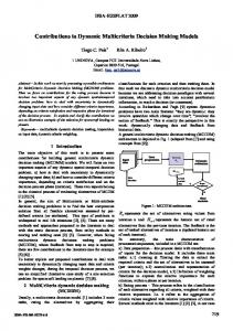
Figure 3.1: The ’binland’ example for a discrete partially ordered landscape. The left figure visualizes the Hamming neighborhood on {0, 1}4 as adjacency graph. choice of neighborhood system may influence the difficulty of an optimization problem significantly. Moreover, we note that the definition of neighborhood gives rise to many characterizations of functions, such as local optimality and barriers. Especially in discrete spaces the neighborhood structure needs to be mentioned then, while in continuous optimization locality mostly refers to the Euclidean metric. The definition of landscape is useful to distinguish the general concept of a function from the concept of a function with a neighborhood defined on the search space and a (partial) order defined on the objective space. We define (poset valued) landscapes as follows: Hasse diagram of the Pareto order for the leading ones trailing zeros (LOTZ) problem. The first objective is to maximize the number of leading ones in the bitstring, while the second objective is to maximize the number of trailing zeros. The preorder on {0, 1} is then defined by the Pareto dominance relation. In this example all local minima are also global minima. Definition 3.1.1 A poset valued landscape is a quadruple L = (X , N, f, �) with X being a set and N a neighborhood system defined on it (e.g. a metric). f : X → Rm is a vector function and � a partial order defined on Rm . The function f : X → Rm will be called height function. An example for a poset-valued landscape is given in the Figure 3.8 and Figure 3.2. Here the neighborhood system is defined by the Hamming distance. It gets obvious that in order to define a landscape in finite spaces we 28
Figure 3.2: Hasse diagram of the Pareto order for the leading ones trailing zeros (LOTZ) problem. The first objective is to maximize the number of leading ones in the bitstring, while the second objective is to maximize the number of trailing zeros. The preorder on {0, 4}2 is then defined by the Pareto dominance relation. In this example all local minima are also global minima (compare figure 3.8). need two essential structures. A neighborhood graph in search space (where edges connect nearest neighbors) the Hasse diagram on the objective space. Note, that for many definitions related to optimization we do not have to specify a height function and it suffices to define an order on the search space. For concepts like global minima the neighborhood system is not relevant either. Therefore, this definition should be understood as a kind of superset of the structure we may refer to in multicriteria optimization.
3.2
Global Pareto Fronts and Efficient Sets
Given f : S → Rm . Here we write f instead of (f1 , . . . , fm )⊤ . Consider an optimization problem: f(x) → min, x ∈ X (3.1) Recall that the Pareto front and the efficient set are defined as follows (Section 1.4): Definition 3.2.1 Pareto front and efficient set
29
The Pareto front YN is defined as the set of non-dominated solutions in Y = f(X ), i. e. YN = {y ∈ Y | ∄y′ ∈ Y : y′ ≺ y}. The efficient set is defined as the pre-image of the Pareto-front, XE = f −1 (YN ). Note, that the cardinality XE is at least as big as YN , but not vice versa, because there can be more than one point in XE with the same image in YN . The elements of XE are termed efficient points. In some cases it is more convenient to look at a direct definition of efficient points: Definition 3.2.2 A point x(1) ∈ X is efficient, iff 6 ∃x(2) ∈ X : x(2) ≺ x(1) . Again, the set of all efficient solutions in X is denoted as XE . Remark Efficiency is always relative to a set of solutions. In future, we will not always consider this set to be the entire search space of an optimization problem, but we will also consider the efficient set of a subset of the search space. For example the efficient set for a finite sample of solutions from the search space that has been produced so far by an algorithm may be considered as a temporary approximation to the efficient set of the entire search space.
3.3
Weak efficiency
Besides the concept of efficiency also the concept of weak efficiency, for technical reasons, is important in the field of multicriteria optimization. For example points on the boundary of the dominated subspace are often characterized as weakly efficient solutions though they may be not efficient. Recall the definition of strict domination (Section 1.4): Definition 3.3.1 Strict dominance Let y(1) , y(2) ∈ Rm denote two vectors in the objective space. Then y(1) (1) strictly dominates y(2) (in symbols: y(1) < y(2) ), iff ∀i = 1, . . . , m : yi < (2) yi . Definition 3.3.2 Weakly efficient solution A solution x(1) ∈ X is weakly efficient, iff 6 ∃x(2) ∈ X : f(x(2) ) < f(x(1) ). The set of all weakly efficient solutions in X is called XwE .
30
x2
f2 f
2
2 efficient
1
non−dominated weakly non−dominated 1 weakly efficient
non−dominated
efficient
0 0
1
0
x1
1
2
f1
Figure 3.3: Example for a solution set containing weakly efficient solutions. Example In Fig. 3.3 we graphically represent the efficient and weakly efficient set of the following problem: f = (f1 , f2 ) → min, S = X = [0, 2] × [0, 2], where f1 and f2 are as follows: � 2 + x1 if 0 ≤ x2 < 1 f1 (x1 , x2 ) = , f2 (x1 , x2 ) = 1+x1 , x1 ∈ [0, 2], x2 ∈ [0, 2]. 1 + 0.5x1 otherwise . The solutions (x1 , x2 ) = (0, 0) and (x1 , x2 ) = (0, 1) are efficient solutions of this problem, while the solutions on the line segments indicated by the bold line segments in the figure denote weakly efficient solutions. Note, that both efficient solutions are also weakly efficient, as efficiency implies weak efficiency.
3.4
Characteristics of Pareto Sets
There are some characteristic points on a Pareto front: Definition 3.4.1 Given an multi-objective optimization problem with m objective functions and image set Y: The ideal solution is defined as y = (min y1 , . . . , min ym ). y∈Y
y∈Y
Accordingly we define the maximal solution: y = (max y1 , . . . , max ym ). y∈Y
y∈Y
31
f2
Maximal point y Y = f(X ) Minimum for f1
Ideal point y
Nadir Point yN
Minimum for f2 f1
Figure 3.4: Ideal points, Nadir point, and maximal point for a multi-objective optimization problem. The Nadir point is defined: yN = (max y1 , . . . , max ym ). y∈YN
y∈YN
For the Nadir only points from the Pareto front YN are considered, while for the maximal point all points in Y are considered. The latter property makes it, for dimensions higher than two (m > 2), more difficult to compute the Nadir point. In that case the computation of the Nadir point cannot be reduced to m single criterion optimizations. A visualization of these entities in a 2-D space is given in figure 3.4.
3.5
Optimality conditions based on level sets
Level sets can be used to visualize XE , XwE and XsE for continuous spaces and obtain these sets graphically in the low-dimensional case: Let in the following definitions f be a function f : S → R, for instance one of the objective functions: Definition 3.5.1 Level sets L≤ (f (ˆ x)) = {x ∈ X : f (x) ≤ f (ˆ x)} 32
(3.2)
Definition 3.5.2 Level curves L= (f (ˆ x)) = {x ∈ X : f (x) = f (ˆ x)}
(3.3)
Definition 3.5.3 Strict level set L< (f (ˆ x)) = {x ∈ X : f (x) < f (ˆ x)}
(3.4)
ˆ ∈ X is (strictly, weakly) Level sets can be used to determine whether x non-dominated or not. ˆ can only be efficient if its level sets intersect in level curves. The point x T Tm Theorem 3.5.4 x is efficient ⇔ m L (f (x)) = ≤ k k=1 k=1 L= (fk (x))
ˆ is efficient ⇔ there is no x such that both fk (x) ≤ fk (ˆ Proof: x x) for all k = 1, . . . , m and fk (x) < f (ˆ x) for at least one k = 1, . . . , m ⇔ there is no m x ∈ X such that both x ∈ ∩ x)) and x ∈ L< (fj (ˆ x)) for some j ⇔ k=1 L≤ (f (ˆ Tm Tm x)) = k=1 L= (fk (ˆ x)) k=1 L≤ (fk (ˆ
ˆ can only be weakly Theorem 3.5.5 The point x Tm efficient if its strict level sets do not intersect. x is weakly efficient ⇔ k=1 L< (fk (x)) = ∅ ˆ can only be strictly efficient Theorem 3.5.6 The point x if its level sets T intersect in exactly one point. x is strictly efficient ⇔ m L k=1 ≤ (fk (x)) = {x}
Level sets have a graphical interpretation that helps to geometrically understand optimality conditions and landscape characteristics. Though this intuitive geometrical interpretation may only be viable for lower dimensional spaces, it can help to develop intuition about problems in higher dimensional spaces. The visualization of level sets can be combined with the visualization of constraints, by partitioning the search space into a feasible and infeasible part. The following examples will illustrate the use of level sets for visualization:
Example Consider the problem f1 (x1 , x2 ) = (x1 −1.75)2 +4(x2 −1)2 → min, f2 (x1 , x2 ) = (x1 − 3)2 + (x2 − 1)2 → min, (x1 , x2 )⊤ ∈ R2 . The level curves of this problem are depicted in Figure 3.5 together with the two marked points p1 and p2 that we will study now. For p1 it gets clear from Figure 3.6 that it is an efficient point as it cannot be improved in both objective function values at the same time. On the other hand p2 is no level point as by moving it to the region directly left of it can be improved in all objective function values at the same time. Formally, the existence of such a region follows from the non-empty intersection of L< (f1 (p2 )) and L< (f2 (p2 )). 33
x2
p1
1
f2 ≡ 0.5 f2 ≡ 1 f2 ≡ 2 f2 ≡ 3
f1 ≡ 1 f1 ≡ 2 f1 ≡ 3 0
1
p2
3
2
x1
Figure 3.5: Representation of two objective functions as level sets. x2
p1
1
L≤ (f1 (p1 )) f1 ≡ 1
0
1
L≤ (f2 (p1 )) f2 ≡ 1
2
3
x1
Figure 3.6: The situation for p1 . In order to improve f1 the point p1 has to move into the set L≤ (f1 (p1 )) and in order to improve f2 it needs to move into L≤ (f1 (p1 )). Since these sets only meet in p1 , it is not possible to improve f1 and f2 at the same time.
34
x2
2 11111111111111111 00000000000000000 00000000000000000 11111111111111111
11111111111111111 00000000000000000 00000000000000000 11111111111111111 00000000000000000 11111111111111111 00000000000000000 11111111111111111 p2 00000000000000000 11111111111111111 00000000000000000 11111111111111111 00000000000000000 11111111111111111 f2 ≡ 3 00000000000000000 11111111111111111 00000000000000000 f1 ≡ 1 00000000000000000 11111111111111111 1 11111111111111111 00000000000000000 11111111111111111 00000000000000000 11111111111111111 00000000000000000 11111111111111111 f2 ≡ 2 00000000000000000 11111111111111111 00000000000000000 11111111111111111 f2 ≡ 1 p1 00000000000000000 11111111111111111 00000000000000000 11111111111111111 00000000000000000 11111111111111111 f1 ≡ 2 00000000000000000 11111111111111111 00000000000000000 11111111111111111 00000000000000000 11111111111111111
0
1
2
x1
3
Example Consider the search space S = [0, 2] × [0, 3]. Two objectives f1 (x1 , x2 ) = 2 + 13 x2 − x1 → min, f2 (x1 , x2 ) = 21 x2 + 12 x1 → max, In addition the constraint g(x1 , x2 ) = − 23 x1 − x2 ≥ 0 needs to be fulfilled. To solve this problem, we mark the constrained region graphically. Now, we can check different points for efficiency. For p1 the region where both objectives improve is in the upper triangle bounded by the level curves. As this set is partly feasible, it is possible to find a dominating feasible point and p1 is not efficient. In contrast, for p2 the set of dominating solutions is completely in the infeasible domain, why this point belongs to the efficient set. The complete efficient set in this example lies on the constraint boundary. Generally, it can be found that for linear problems with level curves intersecting in a single point there exists no efficient solutions in the unconstrained case whereas efficient solutions may lie on the constraint boundary in the constrained case.
3.6
Local Pareto Optimality
As opposed to global Pareto optimality we may also define local Pareto optimality. Roughly speaking, a solution is a local optimum, if there is no better solution in its neighborhood. In order to put things into more concrete terms let us distinguish continuous and discrete search spaces: In finite discrete search spaces for each point in the search space X a set 35
of nearest neighbors can be defined by means of some neighborhood function N : X → ℘(X) with ∀x ∈ X : x 6∈ N(x). As an example consider the space {0, 1}n of bit-strings of length n with the nearest neigbors of a bit-string x being the elements that differ only in a single bit, i.e. that have a Hamming distance of 1. Definition 3.6.1 Locally efficient point (finite search spaces) Given a neighborhood function N : X → ℘(X), a locally efficient solution is a point x ∈ X such that 6 ∃x′ ∈ N(x) : x′ ≺ x. Definition 3.6.2 Strictly locally efficient point (finite search spaces) Given a neighborhood function N : X → ℘(X), a strictly locally efficient solution is a point x ∈ X such that 6 ∃x′ ∈ N(x) : x′ � x. Remark: The comparison of two elements in the search space is done in the objective space. Therefore, for two elements x and x′ with x � x′ and x � x′ it can happen that x 6= x′ (see also the discussion of the antisymmetry property in chapter 2). This definition can also be extended for countable infinite sets, though we must be cautious with the definition of the neighborhood function there. For the Euclidean space Rn , the notion of nearest neighbors does not make sense, as for every point different from some point x there exists another point different from x that is closer to x. Here, the following criterion can be used to classify local optima: Definition 3.6.3 Open ǫ-ball An open ǫ-ball Bǫ (x) around a point x ∈ Rn is defined as: Bǫ (x) = {x′ ∈ X|d(x, x′ ) < ǫ}. Definition 3.6.4 Locally efficient point (Euclidean search spaces) A point x ∈ Rn in a metric space is said to be a locally efficient solution, iff ∃ǫ > 0 :6 ∃x′ ∈ Bǫ (x) : x′ ≺ x. Definition 3.6.5 Strictly locally efficient point (Euclidean search spaces) A point x ∈ Rn in a metric space is said to be a strictly locally efficient solution, iff ∃ǫ > 0 :6 ∃x′ ∈ Bǫ (x) − {x} : x′ � x. The extension of the concept of local optimality can be done also for subspaces of the Euclidean space, such as box constrained spaces as in definition 1.8. 36
y 7 = 14
y 3 = 11 x(3) = 011
x(5) = 101
= 000
y 2 = 0, 3
x(6) = 110
x(4)
y 6 = 1, 2 x(6) = 110
x(2) = 010
y 4 = 15
y0 = 0
x(5) = 101
y 6 = 10
x(2) = 010
y 5 = 5, 4
x(1) = 001
y 2 = 11
x(7) = 111
y 1 = 1, 2
y 5 = 12
x(1) = 001
x(0)
x(3) = 011
x(7) = 111
y 1 = 11
y 7 = 2, 2
y 3 = 2, 1
y 4 = 1, 5
y 0 = 2, 2 x(0)
= 100
= 000
x(4)
= 100
Figure 3.7: Pseudoboolean landscapes with search space {0, 1}3 and the Hamming neighborhood defined on it. The linearly ordered landscape on the right hand side has three local optima. These are x(0) = 000, x(4) = 100, x(7) = 111. x(0) is also a global minimum and x(4) a global maximum. The partially ordered landscape on the right hand side has locally efficient solutions are x(1) = 001, x(2) = 010, x(3) = 011, x(6) = 110. The globally efficient solutions are x(1) , x(2) and x(3)
37
3.7
Barrier Structures
Local optima are just one of the many characteristics we may discuss for landscapes, i.e. functions with a neighborhood structure defined on the search space. Looking at different local optimal of a landscape we may ask ourselves how these local optimal are separated from each other. Surely there is some kind of barrier in between, i.e. in order to reach one local optimum from the other following a path of neighbors in the search space we need to put up with encountering worsening of solutions along the path. We will next develop a formal framework on defining barriers and their characteristics and highlight an interesting hierarchical structure that can be obtained for all landscapes - the so called barrier tree of totally ordered landscapes, which generalizes to a barrier forest in partially ordered landscapes. For the sake of clarity let us introduce formal definitions first for landscapes with a one-dimensional height function as they are discussed in singleobjective optimization. Definition 3.7.1 Path in discrete spaces Let N : X → ℘(X) be a neighborhood function. A sequence p1 , . . . , pl for some l ∈ N and p1 , . . . , pl ∈ S is called a path connecting x1 and x2 , iff p1 = x1 , pi+1 ∈ N(pi ), for i = 1, . . . , l − 1, and pl = x2 . Definition 3.7.2 Path in continuous spaces For continuous spaces a path is a continuous mapping p[0, 1] → X with p(0) = x1 and p(1) = x2 . Definition 3.7.3 Let Px1 ,x2 denote the set of all paths between x1 and x2 . Definition 3.7.4 Let the function value of the lowest point separating two local minima x1 and x2 be defined as fˆ(x1 , x2 ) = minp∈Px1 ,x2 maxx3 ∈p f (x3 ). Points s on some path p ∈ Px1 ,x2 for which f (s) = fˆ(x1 , x2 ) are called saddle points between x1 and x2 . Example In the example given in Figure 3.8 the search points are labeled by their heights, i.e. x1 has height 1 and x4 has height 4. The saddle point between the local minima x1 and x2 is x12 . The saddle point x3 and x5 is x18 .
38
Figure 3.8: Example of a discrete landscape. The height of points is given by the numbers and their neighborhood is expressed by the edges. Lemma 3.7.5 For non-degenerate landscapes, i.e. landscapes where for all x1 and x2 : f (x1 ) 6= f (x2 ), saddle points between two given local optima are unique. Note. that in case of degenerate landscapes, i.e. landscapes where there are at least two different points which share the same value of the height function, saddle points between two given local optima are not necessarily unique anymore, which, as we will see later, influences the uniqueness of barrier trees characterizing the overall landscape. Definition 3.7.6 The valley (or: basin) below a point s is called B(s) : B(s) = {x ∈ S|∃p ∈ Px,s : maxz∈p f (z) ≤ f (s)} Example In the aforementioned example given in Figure 3.8, Again, search points x1 , . . . , x20 are labeled by their heights, i.e. x4 is the point with height 4, etc.. The basin below x1 is given by the empty set, and the basin below x14 is {x1 , x11 , x4 , x9 , x7 , x13 , x5 , x8 }. Points in B(s) are mutually connected by paths that never exceed f (s). At this point it is interesting to compare the level set L≤ (f (x)) with the 39
basin B(x). The connection between both concepts is: Let B be the set of connected components of the level set L≤ (f (x)) with regard to the neighborhood graph of the search space X , then B(x) is the connected component in which x resides. Theorem 3.7.7 Suppose for two points x1 and x2 that f (x1 ) ≤ f (x2 ). Then, either B(x1 ) ⊆ B(x2 ) or B(x1 ) ∩ B(x2 ) = Ø. � Theorem 3.7.7 implies that the barrier structure of a landscapes can be represented as a tree where the saddle points are the branching points and the local optima are the leaves. The flooding algorithm (see Algorithm 2) can be used for the construction of the barrier tree in discrete landscapes with finite search space X and linearly ordered search points (e.g. by means of the objective function values). Note, that if the height function is not injective the flooding algorithm can still be used but the barrier tree may not be uniquely defined. The reason for this is that there are different possibilities of how to sort elements with equal heights in line 1 of algorithm 2. Finally, let us look whether concepts such as saddle points, basins, and barrier trees can be generalized in a meaningful way for partially ordered landscapes. Flamm and Stadler [8] recently proposed one way of generalizing these concepts. We will review their approach briefly and refer to the paper for details. Adjacent points in linearly ordered landscapes are always comparable. This does not hold in general for partially ordered landscapes. We have to modify the paths p that enter the definition. Definition 3.7.8 Maximal points on a path The set of maximal points on a path p is defined as σ(p) = {x ∈ p|∄x′ ∈ p : f (x) ≺ f (x′ )} Definition S 3.7.9 Poset saddle-points Σx1 ,x2 = p∈Px ,x σ(p) is the set of maximal elements along all possible 1 2 paths. Poset-saddle points are defined as the Pareto optima1 of Σx1 ,x2 : S(x1 , x2 ) := {z ∈ Σx1 ,x2 |∄u ∈ Σx1 ,x2 : f (u) ≺ f (z)} The flooding algorithm can be modified in a way that incomparable elements are not considered as neighbors (’moves to incomparable solutions are disallowed’). The flooding algorithm may then lead to a forest instead 1
here we think of minimization of the objectives.
40
Figure 3.9: A barrier tree of a 1-D continuous function. of a tree. For examples (multicriteria knapsack problem, RNA folding) and further discussion of how to efficiently implement this algorithm the reader is referred to [8]. A barrier tree for a continuous landscape is drawn in Fig. 3.9. In this case the saddle points correspond to local maxima. For continuous landscapes the concept of barrier trees can be generalized, but the implementation of flooding algorithms is more challenging due to the infinite number of points that need to be considered. Discretization could be used to get a rough impression of the landscape’s geometry.
3.8
Shapes of Pareto Fronts
An interesting, since very general, questions could be: How can the geometrical shapes of Pareto fronts be classified. We will first look at some general descriptions used in literature on how to define the Pareto front w.r.t. convexity and connectedness. To state definitions in an unambiguous way we will make use of Minkowski sums and cones as defined in chapter 2. Definition 3.8.1 A set Y ⊆ Rm is said to be cone convex w.r.t. the positive orthant, iff YN + Rm ≥ is a convex set. Definition 3.8.2 A set Y ⊆ Rm is said to be cone concave w.r.t. the positive 41
Algorithm 2 Flooding algorithm 1: Let x(1) , . . . , x(N ) denote the elements of the search space sorted in ascending order. 2: i → 1; B = ∅ 3: while i ≤ N do 4: if N(xi ) ∩ {x(1) , . . . , x(i−1) } = ∅ [i. e., x(i) has no neighbour that has been processed.] then 5: {x(i) is local minimum} 6: Draw x(i) as a new leaf representing basin B(x(i) ) located at the height of f in the 2-D diagram 7: B ← B ∪ {B(x(i) )} {Update set of basins} 8: else 9: Let T (x(i) ) = {B(x(i1 ) ), . . . , B(x(iN ) )} be the set of basins B ∈ B with N(x(i) ) ∩ B 6= ∅. 10: if |T (x(i) )| = 1 then 11: B(x(i1 ) ) ← B(x(i1 ) ) ∪ {x(i) } 12: else 13: {x(i) is a saddle point} 14: Draw x(i) as a new branching point connecting the nodes for B(x(i1 ) ), . . . , B(x(iN ) ). Annotate saddle point node with B(x(i) ) and locate it at the height of f in the 2-D diagram 15: {Update set of basins} 16: B(x(i) ) = B(x(i1 ) ) ∪ · · · ∪ B(x(iN ) ) ∪ {x(i) } 17: Remove B(x(i1 ) ), . . . , B(x(iN ) ) from B 18: B ← B ∪ {B(x(i) )} 19: end if 20: end if 21: end while
42
Figure 3.10: Different shapes of Pareto fronts for bi-criteria problems.
43
orthant, iff YN − Rm ≥ is a convex set. Definition 3.8.3 A Pareto front YN is said to be convex (concave), iff it is cone convex (concave) w.r.t. the positive orthant. Note, that Pareto fronts can be convex, concave, or may consist of cone convex and cone concave parts w.r.t. the positive orthant. Convex Pareto fronts allow for better compromise solutions than concave Pareto fronts. In the ideal case of a convex Pareto front, the Pareto front consists only on a single point which is optimal for all objectives. In this situation the decision maker can choose a solution that satisfies all objectives at the same time. The most difficult situation for the decision maker arises, when the Pareto front consists of a separate set of points, one point for each single objective, and these points are separate and very distant from each other. In such a case the decision maker needs to make a either-or decision. Another classifying criterion of Pareto fronts is connectedness. Definition 3.8.4 A Pareto front YN is said to be connected, if and only if for all y1 , y2 ∈ YN there exists a continuous mapping φ : [0, 1] → YN with φ(0) = y1 and φ(1) = y2 . For the frequently occurring case of two objectives, examples of convex, concave, connected and disconnected Pareto fronts are given in Fig. 3.10. Two further corollaries highlight general characteristics of Pareto-fronts:
44
Lemma 3.8.5 Dimension of the Pareto front Pareto fronts for problems with m-objectives are subsets or equal to m−1dimensional manifolds. Lemma 3.8.6 Functional dependencies in the Pareto front Let YN denote a Pareto front for some multiobjective problem. Then for any sub-vector in the projection to the coordinates in {1, . . . , m} without i, the value of the i-th coordinate is uniquely determined. Example For a problem with three objectives the Pareto front is a subset of a 2-D manifold that can be represented as a function from the values of the • first two objectives to the third objective. • the first and third objective to the second objective • the last two objectives to the first objective
45
Chapter 4 Optimality conditions for differentiable problems In the finite discrete case local optimality of a point x ∈ X can be done by comparing it to all neighboring solutions. In the continuous case this is not possible, For differentiable problems we can state conditions for local optimality. We will start with looking at unconstrained optimization, then provide conditions for optimization with equality and inequality constraints and, thereafter, their extensions for the multiobjective case.
4.1
Linear approximations
A general observation we should keep in mind when understanding optimization conditions for differentiable problems is that continuously differentiable functions f : Rn → R can be locally approximated at any point x(0) by means of linear approximations f (x(0) ) + ∇f (x(0) )(x − x0 ) with ∂f ∂f ⊤ ∇f = ( ∂x , . . . , ∂x ) . In other words: n 1 lim f (x) − [f (x0 ) + ∇f (x)(x − x0 )] = 0
x→x0
(4.1)
The gradient ∇f (x(0) ) points in the direction of steepest ascent and is ˆ . This has been visuorthogonal to the level curves L= (f (ˆ x)) at the point x alized in Fig. 4.1.
46
Figure 4.1: Level curves of a continuously differentiable function. Locally the function ’appears’ to be a linear function with parallel level curves. The gradient vector ∇f (ˆ x) is perpendicular to the local direction of the level ˆ. curves at x
4.2
Unconstrained Optimization
For the unconstrained minimization f (x) → min
(4.2)
problem, a well known result from calculus is: Theorem 4.2.1 Fermat’s condition Given a differentiable function f . Then ∇f (x∗ ) = 0 is a necessary condition for x∗ to be a local extremum. Points with ∇f (x∗ ) = 0 are called stationary points. A sufficient condition for x∗ to be a (strict) local minimum is given, if in addition the Hessian matrix ∇2 f (x∗ ) is positive (semi)definite. The following theorem can be used to test wether a matrix is positive (semi)definite: Theorem 4.2.2 A matrix is positive (semi-)definite, iff all eigenvalues are positive (non-negative). Alternatively, we may use local bounds to decide whether we have obtained a local or global optimum. For instance, for the problem min(x,y)∈R2 (x− 47
3)2 + y 2 + exp y the bound of the function is zero and every argument for which the function reaches the value of zero must be a global optimum. As the function is differentiable the global optimum will be also be one of the stationary points. Therefore we can find the global optimum in this case by looking at all stationary points. A more general way of looking at boundaries in the context of optimum seeking is given by the Theorem of Weierstrass discussed in [9]. This theorem is also useful for proving the existence of an optimum. This is discussed in detail in [1]. Theorem 4.2.3 Theorem of Weierstrass Let X be some closed1 and bounded subset of Rn , let f : X → R denote a continuous function. Then f attains a global maximum and minimum in X , i. e. ∃xmin ∈ X : ∀x′ ∈ X : f (xmin ) ≤ f (x′ ) and ∃xmax ∈ X : ∀x′ ∈ X : f (xmax ) ≥ f (x′ ).
4.3
Equality Constraints
By introducing Lagrange multipliers, theorem 4.2.1 can be extended to problems with equality constraints, i. e.: f (x) → min, s.t. g1 (x) = 0, . . . , gm (x) = 0
(4.3)
In this case the following theorem holds: Theorem 4.3.1 Let f and g1 , . . . , gm denote differentiable functions. Then a necessary condition for x∗ to be a local extremum is given, if there exist multipliers λP 1 , . . . , λm+1 with at least one λi 6= 0 for i = 1, . . . , m such that ∗ ∗ λ1 ∇f (x ) + m+1 i=2 λi ∇g(x ) = 0.
For a rigorous proof of this theorem we refer to [1]. Let us remark, that the discovery of this theorem by Lagrange preceded its proof by one hundred years [1]. Next, by means of an example we will provide some geometric intuition for this theorem. In Fig. 4.2 a problem with a search space of dimension two is given. A single objective function f has to be maximized, and the sole constraint function g1 (x) is set to 0. 1
Roughly speaking, a closed set is a set which includes all points at its boundary.
48
x2 −15 −14 −13 ∇g1 (x∗ ) x∗ f ≡ const ∗
∇f (x )
g ≡ const
x1 Figure 4.2: Lagrange multipliers: Level-sets for a single objective and single active constraint and search space R2 . Let us first look at the level curve f ≡ −13. This curve does not intersect with the level curve g ≡ 0 and thus there is no feasible solution on this curve. Next, we look at f ≡ −15. In this case the two curve intersects in two points with g ≡ 0. However, these solutions are not optimal. We can do better by moving to the point, where the level curve of f ≡ c ’just’ intersects with g ≡ 0. This is the tangent point x∗ with c = f (x∗ ) = −14. The tangential point satisfies the condition that the gradient vectors are collinear to each other, i.e. ∃λ 6= 0 : λ∇g(x∗) = ∇f (x∗ ). In other words, the tangent line to the f level curve at a touching point is equal to the tangent line to the g ≡ 0 level curve. Equality of tangent lines is equivalent to the fact that the gradient vectors are collinear. Another way to reason about the location of optima is to check for each point on the constraint curve whether it can be locally improved or not. For points where the level curve of the objective function intersects with 49
the constraint function, we consider the local linear approximation of the objective function. In case of non-zero gradients, we can always improve the point further. In case of zero gradients we already fulfill conditions of the theorem by setting λ1 = 1 and λi = 0 for i = 2, . . . , m + 1. This way we can exclude all points but the tangential points and local minima of the objective function (unconstrained) from consideration. In practical optimization often λ1 is set to 1. Then the equations in the lagrange multiplier theorem boil down to an equation system with m + n unknowns and m + n equations and this gives rise to a set of candidate solutions for the problem. This way of solving an optimization problem is called the Lagrange multiplier rule.
50
Example Consider the following problem: f (x1 , x2 ) = x21 + x22 → min
(4.4)
, with equality constraint g(x1 , x2 ) = x1 + x2 − 1 = 0
(4.5)
Due to the theorem of 4.3.1, iff (x1 , x2 )⊤ is a local optimum, then there exist λ1 and λ2 with (λ1 , λ2 ) 6= (0, 0) such that the constraint in equation 4.5 is fulfilled and ∂f ∂g λ1 + λ2 = 2λ1 x1 + λ2 = 0 (4.6) ∂x1 ∂x1 ∂f ∂g λ1 + λ2 = 2λ1 x2 + λ2 = 0 (4.7) ∂x2 ∂x2 Let us first examine the case λ1 = 0. This entails: λ2 = 0
(4.8)
This contradicts the condition that (λ1 , λ2 ) 6= (0, 0). We did not yet prove, that the solution we found is also a global optimum. In order to do so we can invoke Weierstrass theorem, by first reducing the problem to a problem with a reduced search space, say: f|A → min A = {(x1 , x2 )||x1 | ≤ 10 and |x2 | ≤ 10 and x1 + x2 − 1 = 0}
(4.9) (4.10)
For this problem a global minimum exists, due to the Weierstrass theorem (the set A is bounded and closed and f is continuous). Therefore, the original problem also has a global minimum in A, as for points outside A the function value is bigger than 199 and in A there are points x ∈ A where f (x1 , x2 ) < 199. The (necessary) Lagrange conditions, however, are only satisfied for one point in R2 which consequently must be the only local minimum and thus it is the global minimum. Now we consider the case λ1 = 1. This leads to the conditions: 2x1 + λ2 = 0
(4.11)
2x2 + λ2 = 0
(4.12)
51
f(x1,x2) 0.4 0.35 0.3 0.25 0.2 0.15 0.1 0.05 0 -0.05 -0.1 -0.15
0.4 0.35 0.3 0.25 0.2 0.15 0.1 0.05 0 -0.05 -0.1 -0.15 0.4 0.2 -0.4
0
-0.2
0 x1
-0.2 0.2
0.4
x2
-0.4
Figure 4.3: The level curves of x21 − x32 . The level curve through (0, 0)T is cusp. and hence x1 = x2 . From the equality condition we get: From the constraint it follows x1 + x1 = 1, which entails x1 = x2 = 12 . Another possibility to solve this problem is by means of substitution: x1 = 1 − x2 and the objective function can then be written as f (1 − x2 , x2 ) = (1 −x2 )2 + x22 . Now minimize the unconstrained ’substitute’ function h(x2 ) = (1 − x2 )2 + x22 . ∂h = −2(1 − x2 ) + 2x2 = 0. This yields x2 = 12 . The second x2 derivative
∂2f ∂ 2 x2
= 4. This means that the point is a local minimum.
However, not always all candidate solutions for local optima are captured this way as the case λ1 = 0 may well be relevant. Brinkhuis and Tikhomirov [1] give an example of such a ’bad’ case: Example Apply the multiplier rule to f0 (x) → min, x21 − x32 = 0: The Lagrange equations hold at xˆ with λ0 = 0 and λ1 = 1. An interesting observation is that the level curves are cusp in this case at xˆ, as visualized in Fig. 4.3.
52
4.4
Inequality Constraints
For inequality constraints the Karush Kuhn Tucker conditions are used as optimality criterion: Theorem 4.4.1 The Karush Kuhn Tucker conditions are said to hold for x∗ , if there exist multipliers λ1 ≥ 0, . . . , λm+1 ≥ 0 and at least one λi > 0 for i = 1, . . . , m + 1, such that: ∗
λ1 ∇f (x ) +
m X
λi+1 ∇gi (x∗ ) = 0
(4.13)
i=1
λi+1 gi (x∗ ) = 0, i = 1, . . . , m
(4.14)
Theorem 4.4.2 Karush Kuhn Tucker Theorem (Necessary conditions for smooth, convex programming:) Assume the objective and all constraint functions are convex in some ǫneighborhood of x∗ , If x∗ is a local minimum, then there exiss λ1 , . . . , λm+1 such that KKT conditions are fulfilled. Theorem 4.4.3 The KKT conditions are sufficient for optimiality, provided λ1 = 1. In this case x∗ is a local minimum. Note that if x∗ is in the interior of the feasible region (a Slater point), all gi (x) < 0 and thus λ1 > 0. The next examples discuss the usage of the Karush Kuhn conditions: Example In order to get familiar with the KKT theorem we apply it to a very simple situation (solvable also with high school mathematics). The task is: 1 − x2 → min, x ∈ [−1, 3]2 (4.15) First, write the task in its standard form: f (x) = 1 − x2 → min
(4.16)
g1 (x) = −x − 1 ≤ 0
(4.17)
g2 (x) = x − 3 ≤ 0
(4.18)
subject to constraints
53
The existence of the optimum follows from Weierstrass theorem, as (1) the feasible subspace [-1,3] is bounded and closed and (2) the objective function is continuous. The KKT conditions in this case boil down to: There exists λ1 ∈ R, λ2 ∈ + R0 and λ3 ∈ R+ 0 and (λ1 , λ2 , λ3 ) 6= (0, 0, 0) such that λ1
∂f ∂g1 ∂g1 + λ2 + λ3 = −2λ1 x − λ2 + λ3 = 0 ∂x ∂x ∂x λ2 (−x − 1) = 0 λ3 (x − 3) = 0
(4.19) (4.20) (4.21)
. First, let us check whether λ1 = 0 can occur: In this case the three equations (4.19, 4.20, and 4.21) will be: −λ2 + λ3 = 0
(4.22)
λ2 (−x − 1) = 0
(4.23)
λ3 (x − 3) = 0
(4.24)
. and (λ2 , λ3 ) 6= (0, 0), and λi ≥ 0, i = 2, 3. From 4.22 we see that λ2 = λ3 . By setting λ = λ2 we can write λ(−x − 1) = 0
(4.25)
λ(x − 3) = 0
(4.26)
and for the equations 4.23 and 4.24. Moreover λ 6= 0, for (λ, λ) = (λ2 , λ3 ) 6= (0, 0). From this we get that −x − 1 = 0 and x − 3 = 0. Which is a contradiction so the case λ1 = 0 cannot occur – later we shall see that this could have derived by using a theorem on Slater points 4.4.3. Next we consider the case λ1 6= 0 (or equivalently λ1 = 1): In this case the three equations (4.19, 4.20, and 4.21) will be: −2x − λ2 + λ3 = 0
(4.27)
λ2 (−x − 1) = 0
(4.28)
,
54
, and λ3 (x − 3) = 0
(4.29)
We consider four subcases: case 1: λ2 = λ3 = 0. This gives rise to x = 0 case 2: λ2 = 0 and λ3 = 6 0. In this case we get as a condition on x: 2x(x − 3) = 0 and x 6= 0 or equivalently x = 3 case 3: λ2 6= 0 and λ3 = 0. We get from this: −2x(−x − 1) = 0 and x 6= 0 or equivalently x = −1. case 4: λ2 6= 0 and λ3 6= 0. This cannot occur as this gives rise to −x−1 = 0 and x − 3 = 0 (contradictory conditions). In summary we see that a maximum can possibly only occur in x = −1, x = 0 or x = 3. By evaluating f on these three candidates, we see that f attains its global minimum in x = 3 and the value of the global minimum is −8. Note that we invoked also the Weierstrass theorem in the last conclusion: the Weierstrass theorem tells us that the function f has a global minimum in the feasible region ([-1.3]) and KKT (necessary conditions) tell us that it must be one of the three above mentioned candidates.
4.5
Multiple Objectives
For a recent generalization of the Lagrange multiplier rule to multiobjective optimization we refer to [11]. For multicriterion optimisation the KKT conditions can be generalized as follows: Theorem 4.5.1 Fritz John necessary conditions A neccessary condition for x∗ to be a locally efficient point is that there exist vectors λ1 , . . . , λk and υ1 , . . . , υm such that λ ≻ 0, υ ≻ 0 k X
λi ∇fi (x∗ ) −
i=1
m X
υi ∇gi(x∗ ) = 0.
(4.30) (4.31)
i=1
∗
υi gi (x ) = 0, i = 1, . . . , m 55
(4.32)
Figure 4.4: Level curves of the two objectives touching in one point indicate locally Pareto optimal points in the bi-criterion case, provided the functions are differentiable. A sufficient condition for points to be Pareto optima follows: Theorem 4.5.2 Karush Kuhn Tucker sufficient conditions for a solution to be Pareto optimal: Let x∗ be a feasible point. Assume that all objective functions are locally convex and all constraint functions are locally concave, and the Fritz John conditions hold in x∗ , then x∗ is a local efficient point. In the unconstrained case we get the simple condition: Corollary 4.5.3 In the unconstrained case Fritz John neccessary conditions reduce to λ≻0 (4.33) k X
λi ∇fi (x∗ ) = 0.
(4.34)
i=1
In 2-dimensional spaces this criterion reduces to the observation, that either one of the objectives has a zero gradient (neccesary condition for ideal points) or the gradients are collinear as depicted in Fig. 4.4. A detailed description of the conditions for multiobjective optimization is given in [10]. 56
Chapter 5 Scalarization Methods A straightforward idea to recast a multiobjective problem as a single objective problem is to sum up the objectives in an weighted sum and then to maximize/minimize the weighted sum of objectives. More general is the approach to aggregate the objectives to a single objective by a so-called utility function, which does not have to be a linear sum but usually meets certain monotonicity criteria. Techniques that sum up multiple objectives into a single one by mean of an aggregate function are termed scalarization techniques. A couple of questions arise when applying such techniques: • Does the global optimization of the aggregate function always (or in certain cases) result in an efficient point? • Can all solutions on the Pareto front be obtained by varying the (weight) parameters of the aggregate function? • Given that the optimization of the aggregate leads to an efficient point, how does the choice of the weights control the position of the obtained solution on the Pareto front? Section 5.1 starts with linear aggregation (weighted sum) and answers the aforementioned questions for it. The insights we gain from the linear case prepare us for the generalization to nonlinear aggregation in Section 5.2. The expression or modeling of preferences by means of of aggregate functions is a broad field of study called Multi-attribute utility theory (MAUT). An overview and examples are given in Section 5.3. A common approach to solve multicriteria optimization problems is the distance to a reference point 57
method. Here the decision pointer defines an desired ’utopia’ point and minimizes the distance to it. In Section 5.4 we will discuss this method as a special case of a scalarization technique.
5.1
Linear Aggregation
Linear weighting is an straightforward way to summarize objectives. Formally the problem: f1 (x) → min, . . . , fm (x) → min is replaced by:
m X
(5.1)
wi fi (x) → min, w1 , . . . , wm > 0
(5.2)
i=1
A first question that may arise is, whether the solution of problem 5.2 is an efficient solution of problem 5.1. This is indeed the case as points that are non-dominated w.r.t. problem 5.1 are also non-dominated w.r.t. problem 5.2, which follows from: (1)
∀y , y
(2)
m
∈R :y
(1)
≺y
(2)
⇒
m X i=1
(1) yi
0 such that ∀i = 1, . . . , m and ∀x ∈ X satisfying fi (x) < fi (x∗ ), there exists an index j such that fj (x∗ ) < fj (x) and: fi (x∗ ) − fi (x) ≤M fj (x) − fj (x∗ ) The image of a properly efficient point we will term properly non-dominated. The set of all proper efficient points is termed proper efficient set, and its image proper Pareto front. 58
Figure 5.1: The proper Pareto front for a bicriteria problem, for which in addition to many proper Pareto optimal solutions there exist also two nonproper Pareto optimal solutions. Note, that in the bi-criterion case, the efficient points which are Pareto optimal in the Geoffrion sense are those points on the Pareto-front, where the slope of the Pareto front (f2 expressed as a function of f1 ) is finite and nonzero (see Fig. 5.1). The parameter M is interpreted as trade-off. The proper Pareto optimal points can thus be viewed as points with a bounded tradeoff. Theorem 5.1.2 Weighted sum scalarization Let us assume a Pareto optimization problem (Eq. 5.1) with a Pareto front that is cone convex w.r.t. positive orthant (Rm ≥ ). Then for each properly efficient point x ∈ X there P exist weights w1 > 0, . . . , wm > 0 such that x is one of the solutions of m i=1 fi (x) → min. In case of problems with a non-convex pareto front it is not always possible to find weights Pmfor a given proper efficient point x such that x is one of the solutions of i=1 fi (x) → min. A counterexample is given in the following example:
Example In Fig. 5.2 the Pareto fronts of two different bi-criterion problems are shown. The figure on the right hand side shows a Pareto front which is cone convex with respect to the positive orthant. Here the tangential points of the level curves of w1 y1 + w2 y2 are the solutions obtained with linear 59
Figure 5.2: The concave (left) and convex Pareto front (right). aggregation. Obviously, by changing the slope of the level curves by varying one (or both) of the weights, all points on the Pareto front can be obtained (and no other). On the other hand, for the concave Pareto front shown on the right hand side only the extreme solutions at the boundary can be obtained. As the example shows linear aggregation has a tendency to obtain extreme solutions on the Pareto front, and its use is thus problematic in cases where no a-priori knowledge of the shape of the Pareto front is given. However, there exist aggregation functions which have less tendency to obtain extreme solutions or even allow to obtain all Pareto optimal solutions. They will be discussed in the next section.
5.2
Nonlinear Aggregation
Instead of linear aggregation we can use nonlinear aggregation approaches, e.g. compute a product of the objective function value. The theory of utility functions can be viewed as a modeling approach for (non)linear aggregation functions. A utility function assigns to each combination of values that may occur in the objective space a scalar value - the so-called utility. This value is to be maximized. Note that the linear aggregation was to be minimized. Level curves of the utility function are interpreted as indifference curves (see Fig. 5.3). 60
In order to discuss a scalarization method it may be interesting to analyze where on the Pareto front the Pareto optimal solution that is found by maximizing the utility function is located. Similar to the linear weighting function discussed earlier, this is the point where the level curves of the utility (looked upon in descending order) first intersect with the Pareto front (see Fig. 5.4).
5.3
Multi-Attribute Utility Theory
Next, we will discuss a concrete example for the design of a utility function. This example will illustrate many aspects of how to construct utility functions in a practically useful, consistent, and user-friendly way. Example Consider you want to buy a car. Then you may focus on three objectives: speed, price, fuel-consumption. These three criteria can be weighted. It is often not wise to measure the contribution of an objective function to the overall utility in a linear way. A elegant way to model it is by specifying a function that measures the degree of satisfaction. For each possible value of the objective function we specify the degree of satisfaction of this solution on a scale from 0 to 10 by means of a so-called value function. In case of speed, we may demand that a car is faster than 80m/mph but beyond a speed of, say, 180 km/h the increase of our satisfaction with the car is marginal, as we will not have many occasions where driving as this speed gives us advantages. It can also be the case, that the objective is to be minimized. As an example, we consider the price of the car. The budget that we are allowed to spend marks an upper bound for the point where the value function obtains a value of zero. Typically, our satisfaction will grow if the price is decreased until a critical point, where we may no longer trust that the solution is sold for a fair price and we may get suspicious of the offer. The art of the game is then to sum up these objectives to a single utility function. One approach is as follows: Given value functions vi : R → [0, 10], i = 1, . . . , m mapping objective function values to degree of satisfaction values, and their weights wi , i = 1, . . . , m, we can construct the following optimization problem with constraints:
61
Figure 5.3: Utility function for a bi-criterion problem. If the decision-maker has modeled this utility function in a proper way, he/she will be indifferent whether to choose y(2) and y(3) , but prefer y(3) and y(2) to y(1) .
Figure 5.4: The tangential point of the Pareto front with the indifference curves of the utility function U here determines where the solution of the maximization of the utility function lies on the Pareto front.
62
Figure 5.5: The components (value functions) of a multiattribute utility function.
m
1 X U(f(x)) = α wi vi (fi (x)) +β min wi vi (fi (x)), i∈{1,...,m} m i=1 {z } | | {z } minority interest common interest (here: m = 3) s. t. vi (fi (x)) > 0, i = 1, . . . , m
(5.4)
(5.5) (5.6)
Here, we have one term that looks for the ’common interest’. This term can be comparably high if some of the value functions have a very high value and others a very small value. In order to enforce a more balanced solutions w.r.t. the different value functions, we can also consider to focus on the value function which is least satisfied. In order to discard values from the search space, solution candidates with a value function of zero are considered as infeasible by introducing strict inequality constraints. A very similar approach is the use of desirability indices. They have been first proposed by Harrington [13] for applications in industrial quality management. Another well known reference for this approach is [14]. We first give a rough sketch of the method, and then discuss its formal details. As in the previously described approach, we map the values of the objective function to satisfaction levels, ranging from not acceptable (0) to totally satisfied (1). The values in between 0 and one indicate the grey areas. Piecewise defined exponential functions are used to describe the mappings. They can be specified by means of three parameters. The mapped objective function values are now called desirability indices. Harrington proprosed to aggregate these desirability indices by a product expression, the minimization of which leads to the solution of the multiobjective problem. 63
The functions used for the mapping of objective function values to desirability indices are categorized into one-sided and two sided functions. Both have a parameter yimin (lower specification limit), yimax (upper specification limit), li , ri (shape parameters), and ti (symmetry center). The one-sided functions read: yi < yimin 0, � �li min yi −yi Di = (5.7) , yimin < yi < ti min ti −yi 1, yi ≥ ti
and the two sided functions read: 0, yi < yimin � � min li yi −ymin i , yimin ≤ yi ≤ ti ti −yi � �ri Di = yi −yimax , ti < yi ≤ yimax max ti −yi 0, yi > y max
(5.8)
The two plots in Fig. 5.6 visualize one-sided (l) and two-sided (r) desirability indexes.
64
1.5
1.5
f(x) f(x) l=1.5
1
D(y)
D(y)
1
0.5
0
-0.5 -1.5
l=0.5 l=1 l=1.5
0.5
0
-1
-0.5
0
0.5
1
1.5
-0.5 -1.5
y
-1
-0.5
0
0.5
1
1.5
y
Figure 5.6: In the left figure we see and examples for one-sided desirability function with parameters y min = −1, y max = 1, l ∈ {0.5, 1, 1.5}. The left side displays a plot of two sided desirability functions for parameters y min = −1.y max = 1, l ∈ {0.5, 1.0, 1.5}, and r being set to the same value than l. The aggregation of the desirability indices is done by means of a product formula, that is to be maximized: k Y 1 D = ( Di (yi )) k i=1
65
(5.9)
In literature many approaches for constructing non-linear utility functions are discussed. The Cobbs Douglas utility function is widely used in economy. Let fi , i = 1, . . . , m denote non-negative objective functions, then the Cobbs Douglas utility function reads: m Y U(x) = fi (x)αi (5.10) i=1
It is important to note, that for the Cobbs Douglas utility function the objective function values are to be minimized, while the utility is to be maximized. Indeed, the objective function values, the values αi , and the utility have usually an economic interpretation, such as the amount of goods: fi , the utility of a combination of goods: U, and the elasticities of demand: αi . A useful observation is that taking the logarithm of this function transforms it into a linear expression: m X αi log fi (x) (5.11) log U(x) = i=1
The linearity can often be exploited to solve problems related to this utility function analytically. A more general approach for construction of utility functions is the Keeney Raiffa utility function approach [12]. Let fi denote non-negative objective functions: m Y U(x) = K (wi ui (fi (x)) + 1) (5.12) i=1
Here wi are weights for the objective functions between 0 and 1 and K denotes a positive scaling constant. Moreover, ui denote functions that are strictly increasing for positive input values. A general remark on how to construct utility functions is, that the optimization of these functions should lead to Pareto optimal solutions. This can be verified by checking the monotonicity condition for a given utility function U: ∀x, x′ ∈ X : x ≺ x′ ⇒ U(x) > U(x′ )
(5.13)
This condition can be easily verified for the two given utility functions.
66
5.4
Distance to a Reference Point Methods
A special class of utility functions is the distance to the reference point (DRP) method. Here the user specifies an ideal solution (or: utopia point) in the objective space. Then the goal is to get as close as possible to this ideal solution. The distance to the ideal solution can be measured by some distance function, for example a weighted Minkowski distance with parameter γ. This is defined as: m X 1 d(y, y ) = [ wi|yi − yi′ |γ ] γ , γ ≥ 1, w1 > 0, . . . , wm > 0 ′
(5.14)
i=1
Here, wi are positive weights that can be used to normalize the objective function values. In order to analyze which solution is found by means of a DRP method we can interpret the distance to the reference point as an utility function (with the utility value to be minimized). The indifference curves in case of γ = 2 are spheres (or ellipsoids) around the utopia point. For γ > 2 one obtains different super-ellipsoids as indifference curves. Here, a super-ellipsoid around the utopia point f ∗ of radius r ≥ 0 is defined as a set: S(r) = {y ∈ Rm |d(y, f ∗) = r} (5.15) with d : Rm × Rm → R+ 0 being a weighted distance function as defined in Eq. 5.14. Example In Figure 5.7 for two examples of a DRP method it is discussed, how the location of the optimum is obtained geometrically, given the image set f(X ). We look for the super-ellipsoid with the smallest radius that still touches the image set. If two objective functions are considered and weighted Euclidean distance is used, i.e. γ = 2, then the super-ellipsoids are regular ellipses (Fig. 5.7). If instead a manhattan distance (γ = 1) is used with equal weights, then we obtain diamond shaped super-ellipsoids (Fig. 5.7). Not always an efficient point is found when using the DRP method. However, in many practical cases the following sufficient condition can be used in order to make sure that the DRP method yields an efficient point. This condition is summarized in the following lemma:
67
Figure 5.7: Optimal points obtained for two distance to DRP methods, using the weighted Euclidean distance (left) and the manhattan distance (right). Lemma 5.4.1 Let f ∗ ∈ Rm denote an utopia point, then x∗ = arg min d(f(x), f ∗ ) x∈X
(5.16)
is an efficient point, if for all y ∈ f(X ) it holds that f ∗ � y. Often the utopia point is chosen to be zero (for example when the objective functions are strictly positive). Note that it is neither sufficient nor necessary that f ∗ is non-dominated by f(X ). The counterexamples given in Fig. 5.9 confirm this. Another question that may arise, using the distance to a reference point method is whether it is possible to find all points on the Pareto front, by changing the weighting parameters wi of the metric. Even in the case that the utopia points dominates all solutions we cannot obtain all points on the Pareto front by minimizing the distance to the reference in case of γ < ∞. Concave parts of the Pareto front may be overlooked, because we encounter the problems that we discussed earlier in case of linear weighting. However, in case of the weighted Tschebycheff distance (or: maximum distance) ′ d∞ max wi |yi − yi′ | (5.17) w (y, y ) = i∈{1,...,m}
we can obtain all points on the Pareto front by optimizing the distance for different weights wi . In more detail, the following condition is satisfied: ′ ∗ ∀y ∈ YN : ∃w1 , . . . , wm : y ∈ arg min d∞ y (y , f ) ′ y ∈Y
68
Figure 5.8: In the left figure we see and example for a utopia point which is non-dominated by the image set but the corresponding DRP method does not yield a solution on the Pareto front. In the right figure we see an example where an utopia point is dominated by some points of the image set, but the corresponding DRP method yields a solution on the Pareto front. However, by using the Tschebycheff metric we may also obtain dominated points, even in cases where f ∗ dominates all solutions in f(X ). These solutions are then weakly dominated solutions. In summary, distance to a reference point methods can be seen as an alternative scalarization approach to utility function methods with a clear interpretation of results. They require the definition of a target point (that ideally should dominate all potential solutions), and also a metric needs be specified. We note, that the Euclidean metric is not always the best choice. Typically, the weighted Minkowski metric is used as a metric. The choice of weights for that metric and the choice of γ can significantly influence the result of the method. Except for the Tschebycheff metric, it is not possible to obtain all points on a Pareto front by changing the weights of the different criteria. The latter metric, however, has the disadvantage that also weakly dominated points may be obtained.
69
Figure 5.9: In the left figure we see and example where an non-dominated point is obtained using a DRP with the Tschebychev distance. In the right figure we see an example where also dominated solutions minimize the Tschebychev distance to the reference point. In these cases a non-dominated solution may be missed by this DRP method if it returns some single solution minimizing the distance.
70
Chapter 6 Transforming Multicriteria into Constrained Single-Criterion Problems This chapter will highlight two common approaches for transforming Multicriteria into Constrained Single-Criterion Problems. In Compromise Programming (or ǫ-Constraint Method), m − 1 of the m objectives are transformed into constraints. Another approach is put forward in the so-called goal attainment and goal programming method. Here a target vector is specified (similar to the distance to a reference point methods), and a direction is specified. The method searches for the best feasible point in the given direction. For this a costraint programming task is solved.
6.1
Compromise Programming or ǫ-Constraint Methods
In compromise programming we first choose f1 to be the objective function that has to be solved with highest priority and then re-state the original multicriteria optimization problem (Eq. 1.11): f1 (x) → min, f2 (x) → min, . . . , fm (x) → min
(6.1)
into the single-criterion constrained problem: f1 (x) → min, f2 (x) ≤ ǫ2 , . . . , fm (x) → ǫm . 71
(6.2)
Figure 6.1: Compromise Programming in the bi-criteria case. The second objective is transformed into a constraint. In figure 6.1 the method is visualized for the bi-criteria case (m = 2). Here, it can be seen that if the constraint boundary shares points with the Pareto front, these points will be the solutions to the problem in Eq. 6.2. Otherwise, it is the solution that is the closest solution to the constraint boundary among all solutions on the Pareto-front. In many cases the solutions are obtained at points x where all objective function values fi (x) are equal to ǫi for i = 1, . . . , m. In these cases, we can obtain optimal solutions using the Lagrange Multiplier method discussed in chapter 4. Not in all cases the solutions we obtain with the compromise programming method are Pareto optimal. An example for a problematic case is given in figure 6.2. The compromise programming method can be used to approximate the Pareto front. For a m dimensional problem a m−1 dimensional grid needs to be computed that cover the m−1 dimensional projection of the bounding box of the Pareto front. Due to Lemma 3.8.6 given m − 1 coordinates of a Pareto front, the m-th coordinate is uniquely determined as the minimum of that coordinate among all image vectors that have the m − 1 given coordinates. As an example, in a 3-D case (see Figure 6.3) we can place points on a grid 72
Figure 6.2: Problematic case for the compromise programming method in 3-D. The cheese-like cylinder denotes the image set f(X ). The Constraint boundaries are indicated by planes. Note that all objectives are to be maximized. Two of the infinitely many solutions in the image set that qualify as solutions of the constrained problem are indicated by black points. The black point on the right hand side f ∗ ′ dominates the black point on the left hand side f ∗ .
73
Figure 6.3: Compromised Programming used for approximating the Pareto front with 3 objectives. stretching out from the minimal point (f1min , f1max ) to the maximal point (f2min , f2max ) . It is obvious that, if the grid resolution is kept constant, the effort of this method grows exponentially with the number of objective functions m. This method for obtaining a Pareto front approximation is easier to control than the to use weighted scalarization and change the weights gradually. However, the knowledge of the ideal and the Nadir point is needed to compute the approximation, and the computation of the Nadir point is a difficult problem in itself.
74
6.2
Concluding remarks on single point methods
In the last two chapters various approaches have been discussed to reformulate a multiobjective problem into a single-objective or a constrained singleobjective problem. The methods discussed have in common that they result in a single point, why they also are referred to as single point methods. In addition, all single point methods have parameters the choice of which determines the location of the optimal solution. Each of this methods has, as we have seen, some unique characteristics and it different to give a global comparison of them. However, a criterion that can be assessed for all single point methods is, whether they are always resulting in Pareto optimal solutions. Moreover, we investigated whether by changing their parameters all points on the Pareto front can be obtained. To express this in a more formal way we may denote a single point method by a function A : P × C 7→ Rm ∪ {Ω}, where P denotes the space of multiobjective optimization problems, C denotes the parameters of the method (e.g. the weights in linear weighting). In order to classify a method A we introduce the following two definitions: Definition 6.2.1 Proper single point method A method A is called proper, if and only if for all p ∈ P and c ∈ C either p has a solution and the point A(p, c) is Pareto optimal or p has no solution and A(p, c) = Ω. Definition 6.2.2 Exhaustive single point method S A method A is called exhaustive if for all p ∈ P : YN (p) ⊆ c∈C A(p, c), where YN (p) denotes the Pareto front of problem p. The following table summarizes the properties of methods we discussed:
75
Single Point Method Linear Weighting
Proper Yes
Exhaustive No
Weighted Euclidean DRP
No
No
Weighted Tschebyschev DRP
No
Yes
Desirability index
No
No
Goal programming
No
No
Compromise programming
No
Yes
Remarks Exhaustive for convex Pareto fronts with only proper Pareto optima Proper if reference point dominates all Pareto optimal points Weakly non-dominated points can be obtained, even when reference point dominates all Pareto optimal points The classification of proper/exhaustive is not relevant in this case. For convex and concave Pareto fronts with the method is proper and exhaustive if the reference point dominates all Pareto optimal solutions In two dimensional objective spaces the method is proper. Weakly dominated points may qualify as solutions for more than three dimensional objective spaces
In the following chapters on algorithms for Pareto optimization the single point methods often serve as components of methods that compute the entire Pareto front, or an approximation to it.
76
Part I Algorithms for Pareto Optimization
77
Chapter 7 Pareto Front Computing with Deterministic Methods In the previous chapters we looked at ways to reformulate multiobjective optimization problems as single objective (constrained) optimization problems. However, it can be very desirable for the decision maker to know the entire Pareto front. Methods to compute the Pareto front or an finite set approximation to it can be subdivided into deterministic methods that often guarantee convergence to sets consisting of Pareto points. Some of these methods can also compute approximation sets that distribute in a well defined way, e.g. uniformly over the arc length (homotopy or continuation method) or optimality in terms of the coverage of the dominated hypervolume (S-metric gradient). Of course, in any of these cases certain assumptions about the function, such as convexity or continuity, have to hold in order to provide guarantees on the quality of the computed set.
7.1
Continuation methods
Continuation methods are a class of numerical methods that are used to compute uniformly spaced point sets covering the Pareto front. The basic idea is to start with a single Pareto optimal points and then gradually move to points in its environment and thereby extending the covered surface. The difficulty is to find the right direction and step length in the search space that leads to points in a defined distance of existing points. 78
If certain conditions are met, systematic ways to generate neighboring points can be derived. In all cases the connectedness of the Pareto front (in the objective space) is assumed. In addition we assume that one connected component of the efficient set will cover the Pareto front. Next, we will discuss one particular continuation method which will provide all points of a convex 2-D Pareto front. The idea is to first compute with a single-objective optimization method the two extreme points on the Pareto front, say x(0) = arg minn f1 (x)
(7.1)
x(1) = arg minn f2 (x)
(7.2)
x∈R
and x∈R
Next we want to compute a uniformly spaced set of Pareto optimal points on the Pareto front which can be described implicitly as the path x(λ), λ ∈ [0, 1] with x(λ) = arg minn (1 − λ)f1 (x) + λf2 (x) (7.3) x∈R
and, assuming convexity and continuous differentiability, this can be expressed as: (1 − λ)∇f1 (x) + λ∇f2 (x) = 0 (7.4) Note that the extremal points on the Pareto front have as preimages x(0) and x(1). The challenge is now to generate a set of points on the Pareto front with a pre-defined distance to each other. To compute this set we start from x(0) and move successively to neighboring points on the Pareto front, whereby the arclength between neighboring points is approximately given by ∆. Given a point x(λt ) we can compute the next point x(λt+1 ) as follows. First we compute a search direction: ˜ := x(λt + ǫ) − x(λt ) v
(7.5)
x(λt + ǫ) = arg minn (1 − λt − ǫ)f1 (x) + (λt + ǫ)f2 (x)
(7.6)
, where x∈R
and ǫ is an appropriately small positive number. The normalized v := used as the search direction. 79
˜ v ||˜ v||
is
Let F = (f1 , f2 ). We proceed to compute the step size h ∈ R+ along v in the decision space xt+1 = xt + hv such that ||F (xt ) − F (xt+1 ||∞ = Θ∆ (where Θ ∈ (0, 1) is a safety factor). In case F is Lipschitz continuous we know that there exists an L ≥ 0 such that ∀x, x′ ∈ X , ||F (x) − F (x′ )|| ≤ L||x − x′ ||
(7.7)
The Lipschitz constant around xt can be estimated by: 2
Lxt := ||DF (xt)||∞ = max ||∇fi (xt )||1 i=1
(7.8)
Combining 7.7 and 7.8, using h = ||xt − xt+1 ||, and assuming h is sufficiently small, we obtain the following estimate: h≈
Θ∆ Lxt
(7.9)
We can now state how to find the next Pareto optimal point xt+1 . Apply the ǫ-constraint method where the constant ǫ is computed as the second coordinate of the expression ǫ := π2 (F (xt ) + F ′ (hv)) From which we get: xt+1 := arg min f1 (x) such that f2 (x) = ǫ.
80
(7.10)
Bibliography [1] J. Brinkhuis and V. Tikhomirov: Optimization: Insights and Applications, Princeton University Press, NY, 2005. [2] Matthias Ehrgott: Multicriteria Optimization, Springer, 2005 [3] B. A. Davey, H.A. Priestley: Introduction to Lattices and Orders (Second Edition), Cambridge University Press, UK, 1990 [4] B. H. Margolius: Permutations with Inversions, 4, Journal of Integer Sequences, Article 01.1.4 (Electronic Journal),2001 [5] H. J. Pr¨omel, A. Steger, and A. Taraz, Counting partial orders with a fixed number of comparable pairs, Combin. Probab. Comput. 10 (2001) 159177; [6] Steven Finch: Mathematical Constants, Chapter: Transitive Relations, Topologies and Partial Orders, Cambridge University Press, 2003 [7] Jorge Nocedal and Stephen J. Wright: Numerical Optimization (Second Edition), Springer 2007 [8] Stadler, P.F.; Flamm, Ch.: Barrier Trees on Poset-Valued Landscapes, Genet. Prog. Evolv. Mach., 4: 7-20 (2003) [9] Jozef Bialas and Namakura Shinshu: The Theorem of Weierstrass, Journal of Formalized Mathematics, Volume 7 (Online). [10] K. Miettinen: Nonlinear Multiobjective Optimization [11] A. G¨otz and J. Jahn: The Lagrange Multiplier Rule in Set-Valued Optimization: SIAM Journal on Optimization, Volume 10 , Issue 2 (1999)
81
Pages: 331 - 344 Year of Publication: 1999 Kluwer Academic Publishers, Boston, 1999. [12] R.L. Keeney and H. Raiffa: Decisions with multiple objectives: preferences and value tradeoffs, Cambridge University Press, 1993 [13] Harrington, J.: The desirability function; Industrial Quality Control 21 (10). pp. 494-498 [14] Derringer, G.C. and Suich, D.: Simultaneous optimization of several response values, Journal of Quality Technology 12 (4), pp. 214-219
82