Multidimensional Data Streams Summarization Using ... - Lirmm

Multidimensional Data Streams Summarization Using Extended Tilted-Time Windows Yoann Pitarch� �

Anne Laurent�

Marc Plantevit��

Pascal Poncelet�

Montpellier Laboratory of Computer Science, Robotics, and Microelectronics University of Montpellier II - CNRS 161 rue Ada 34392 Montpellier Cedex 5 France {first name.name}@lirmm.fr �� GREYC - CNRS - UMR 6072, University of Caen Campus Cte de Nacre, F-14032 Caen Cedex France {first name.name}@info.unicaen.fr allowing such on-line analysis. Firstly, logs arrive at an intensive rate. As a consequence, the volume of data is huge and it is impossible to store the whole history. Secondly, data registered are too specific to be relevant. For instance, storing the whole history of consulted web pages is not really interresting and a web site administrator would prefer storing the history of most popular sections. Those two characteristics naturally lead us considering logs as data stream. Indeed a stream can be defined as a potentially infinite sequence of data residing at a rather low level and arriving at an intensive rate. Moreover, web logs are composed by several dimensions. For instance a web log server registers visitor’s IP, the date, the status code, ... In most of cases, every dimension can be considered at multiple granularity levels. For instance, status code can also be considered by categories (informational, successfull, redirection, ...). The success of OLAP technology naturally leads to its possible extension from static data to data produced on dynamic environments. So the question is “it is possible to build a datacube and perform on-line analysis on web server logs? ”. To the best of our knowledge, the approach proposed in [4] is the first one proposing to tackle this problem. But even if this approach is promising, two facts have to be taken into account. Firstly, logs are supposed to fit in memory. Secondly, the data cube is built on static data. As a consequence, this approach cannot be applied to the data stream context.

Abstract Nowadays, servers register more and more log entries. Monitoring, analyzing and exctracting knowledge from networks and web servers is crucial for a lot of applications. Indeed, logs can be useful for describing the activity by means of several dimensions. But logs arrive at an intensive rate and are observable at a low level of granularity which make it unrealistic to store the whole log history and leads us considering logs as data stream. Moreover, as logs are composed by several fields which can be considered as multiple levels of granularity, it would be interresting to provide an on-line analytical processing on such data stream. So, a natural question is “it is possible to perform a multi-level and multidimensional analysis by building a cube supplied by a data stream?”. A choice has to be done in order selecting the most useful information. We tackle this problem by exploiting user’s preferences. Generaly, users consult the recent history at fine levels of granularity. Then, this need of precision decreases when the age of the data increases. To this end, we introduce precision functions. Their combination lead to a compact data cube framework which can answer to most of queries. Experiments conduced on both synthetic and real data set show that our approach can be applied to data stream context.

1. Introduction With the rapid development of the World Wide Web the volume of data registered by a web server may be huge. But monitoring, analyzing and exctracting knowledge from networks and web servers is crucial for a lots of applications: performance improvement, web sites improvements, ads placement, ... Indeed, logs can be useful for describing the activity of a web site. But two technical matters have to be tackled to

More recently, StreamCube approach [2] introduces a method to perform multi-dimensional, multi-level, on-line analysis of data streams. This proposition is based on the so-called tilted time frame [1] in order to compress the temporal dimension. This model consists 1

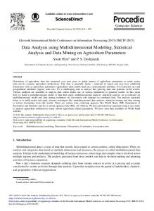
Figure 1: A natural tilted-time window model

in considering time at multiple levels of granularity and will be more described in Section 2.2. Since it is impossible to store all the cuboids, authors propose to store some of them. This choice is led by expert domain knowledge, query history and statistical analysis of the sizes of intermediate cuboids. Even if [2] presents an interesting architecture, two aspects of this proposition are enhanceable. Firstly, data are systematically propagated along of the stored cuboids. This increases the time required to insert an element in the structure. Secondly, this approach keep a track of the old history of the fine granularity levels. This is not necessary because in practice, the fine granularity levels almost are not queried for the whole history of the data stream. In this paper, we improve the StreamCube approach by taking into account its two major drawbacks. The three main contributions of this work are:

2.1. Data Cube Originally, data cubes were introduced to facilitate multi-dimensional and multi-level analysis of large data sets. Let DB be a set of tuples defined on a set of n dimensions denoted by D. This set is called the base table of a cube. The set of all attributes A in D are partitioned in two subsets, the dimensional attributes DIM and the measures attributes M. Note that DIM ∪ M = A and DIM ∩ M = ∅. Every dimension Di ∈ DIM can be considered at multiple levels of granularities. We call these levels and the way they are organized the hierarchy of the dimension Di with the following notations: maxi is the number of levels of the hierarchy with Dimaxi the finest level and Di1 the coarsest. Note that for every dimension Di ∈ DIM we consider a wild-card value * which can be defined as all the values in Di . With these notations, a tuple t is defined as t = (d1 , ..., dn , m1 , .., mk ) such that for every i = 1...m and li = 1...maxi , di ∈ Dom(Dili ) ∪ {∗}, Di ∈ DIM . The measure attributes (m1 , .., mk ) functionally depend on the dimensional attributes in DB and are defined in the context of data cubing using some typical aggregate functions.

• Fine levels of granularity are mostly queried for the recent history. So, we propose to materialize only the required parts of the history for each level of granularity. For example, if a level has never been queried after the most recent month, it is useless to keep a track of it for the rest of the history. Thus, the storage cost per dimension is much more reduced and Precision functions formulate this idea. • Then, we combine these functions to propose a compact framework, which allows multidimensional, multi-level, efficient and on-line analysis of data streams.

2.2. Data Stream A data stream S = B0 , B1 , ..., Bn is an infinite sequence of batches, where each batch is associated with a timestamp t, i.e. Bt , and n is the identifier of the most recent batch Bn . A batch Bi is defined as a set of tuples appearing over the stream at the ith time unit.

• Our experiments conducted on both synthetic and real datasets show the effectiveness and the efficiency of our approach. The rest of the paper is organized as follows. In Section 2, we define the basic concepts and introduce the problem statement. In Section 3 we propose a framework for on-line analysis of stream data by introducing the precision functions as well as their combining. Our experiments and performance studies are presented in Section 4. Future work and conclusion are formulated in Section 5.

The volume of data generated by data streams is too huge to be totally materialized. In stream data analysis, people are usually interested in recent changes at a fine granularity, but long term changes at coarse scale. Thus, the literature proposes a model which takes inspiration of this: the tilted-time window model [1]. In fact, time can naturally be registered at different levels of granularity. The most recent time is registered at the finest granularity and the more distant time is registered at coarser granularity. The level of coarseness depends on the application requirements and on how old the time point is from the current time. Figure 1 provides an example of tilted-time windows.

2. Problem Statement In this Section, we introduce the basic concepts related to data cubes and streams. Then, the ongoing challenge is defined. 2

Table 1: Statistics on level request according to the time

2.3. The Ongoing Challenge On the one hand data cubes require a huge amount of space and on the other both space and time are critical aspects in data stream applications. Our task is to accommodate these constraints in order to support efficient, high-level, on-line, multi-dimensional analysis of data streams. For example, such analysis may enable to discover trends and exceptions according to users’ preferences. This may involve the construction of a data cube in order to facilitate such on-line and flexible analysis.

Level

Interval

Frequency

GEOGRAPHIC DIMENSION IP

City Country

2.4. Motivating Example

[now; t−1 ] [t−1 ; t−2 ] [now; t−1 ] [t−1 ; t−2 ] [t−2 ; t−3 ] [t−3 ; t−4 ] [t−3 ; t−4 ]

98% 2% 25% 40% 34% 1% 100%

[now; t−1 ] [t−1 ; t−2 ] [t−2 ; t−3 ] [t−3 ; t−4 ]

100% 70% 20% 10%

FILE DIMENSION file name

In order to illustrate our previous definitions and our proposition, we consider a stream representing logs registered by a web server. To facilitate the comprehension, we consider that each log contains only two dimensions, Geographic and File. Their respective levels of granularity (excluding the highest level ’*’) are (Country, City, IP ) and (file type, file name). Suppose that a web site administrator wants to keep track of the log history in a compact way but the tilted time model shown in Figure 1 is not sufficient. In order to provide a space-saving framework, the statistics displayed on Table 1 are used. This table provides the query rate per level, depending on the tilted-time window intervals. For example, IP level is only requested on [now; t−1 ]. As a consequence, it is useless to materialize its history after t−1 . Since fine granularity levels are less consulted for the old history, we propose a method materializing only the part of the history which is necessary for users’ queries. Using this toy example, we show how user’s preferences can be exploited to produce a space-saving framework compared to the StreamCube approach [2]: it is unnecessary to materialize data which is never queried. To this end, we introduce precision functions and their combination in order to propose a savespacing data structure which allows efficient, multidimensional and multi-level analysis.

file type

3.1. Precision Function Let us consider Table 1. We see that the level IP is never queried after t−2 . Thus, it is useless to keep a track of web server logs at IP granularity level after t−2 . To this end, we introduce for each granularity level l a value endl which means data are not stored at the granularity level l after endl . Here, we have endIP = t−2 . Let Dip a level of granularity of a dimension Di . In order to define when Dip is no more queried, we introduce the notation endip (endp if there is no ambiguity on the dimension), with endp ∈ t−1 , ..., t−k and end1 = t−k . Note that (1) if p� is a finer level than p, we have endp� < endp and (2) endALL is never defined. The second limit is that data are systematically propagated along of the stored cuboids. It is useless and costly because it introduces redundancy in the framework. For example, if endIP is set to t−2 , it is unnecessary to store the stream history before t−2 for the level City. Indeed, the visitors localisation per cities and countries can be computed thanks to the OLAP roll-up operator. Thus, for a level of granularity Dip , we introduce the notation beginip (beginp if there is no ambiguity on the dimension) defined as beginip = endip+1 with 1 ≤ p < maxi and beginmaxi = t0 .

3. Contribution We start this Section by introducing precision functions which consider that levels of each dimension are not queried for all the history. Then, the combination of these functions leads to a compact and interesting cube model.

Now that we have defined beginp and endp for every level of granularity Dip , we can introduce precision 3

functions as follows:

We describe the way to insert values in the framework. Let us examine Figure 3. While a window is not full and the next window is materialized on the same cuboid, the insertion process is the same than the classical tilted-time window ’s one. The difference takes place when a window is full and the next one is materialized on a upper cell. As shown in Figure 3, a dual aggregation is done. The first aggregation is classical. Then, all the aggregated values of cells which share the same upper cell are aggregated. In the example, the lowest upper cell of (123.123.123.123, map.jpg) and (123.125.127.129, bob.gif ) is (Paris, image). Thus, combined values of both cells are aggregated. In this example, we consider a batch representing daily logs. In the cell (123.125.127.129, bob.gif ), the value 10 means the visitor with IP equals to 123.125.127.129 consulted 10 times the file bob.gif yesterday. The result is displayed on Figure 3.

P rec(Dip ) = [beginp ; endp ] In other words, P rec(Dip ) is the minimal interval required to both satisfy users’ queries and avoid storing computable data. We note that {P rec(Dip ), 0 ≤ p ≤ maxi } forms a partition of T . Example 1 Figure 2 displays precision functions used in the example. If we consider P rec(City) we note that: 1. Since P rec(City) = [t−2 ; t−3 ], web server logs at the city granularity level are physically stored. 2. It is impossible to get a precise information on web site visits per IP between t−2 and t−3 . 3. On the contrary, visits made beetween t−2 and t−3 per country may be obtained by using roll-up operator

Figure 3: Insertion

Figure 2: Graphic representation of precision functions

A good definition of the precision functions is crucial for our model in order to minimize imprecise answers. For example, let us imagine that the level City of the geographic dimension is only stored on the first interval, [now; t−1 ]. This could be critical since 75% of queries relating to this level cannot be answered. As a consequence, users have to define themselves these functions. We present here two solutions for this problem.

4. Performance Study

3.2. Combining Precision Functions

4.1. Experimental Method

We have defined above precision functions for each dimension. Since data are multidimensional, we have to propose a method to combine those functions. A simple and efficient way for performing this is to use intersection. To this end, we define the function Materialize. Let C = D1p1 D2p2 ..Dkpk be a cuboid (with 1 ≤ k ≤ n and 0 ≤ pi ≤ Pmaxi for 1 ≤ i ≤ k). We define the Materialize function as follows: � ∅, M aterialize(C) = �k

We performed an extensive evaluation on both real and synthetic datasets. Our results show that the Random Access Memory and computation time taken by our method are small and bounded. As a consequence, it is realistic to compute and update such a cube in a stream context. In a first time, performance studies conducted on web server logs coming from a french laboratory web server are reported. Then, performance studies on a real data set that gathered from TCP/IP network traffic at the University of Montpellier are displayed.

if k �= n pi P rec(D ), otherwise i i=1 4

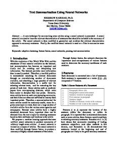
Figure 4: Time consumption results on TCP/IP haeders dataset

approach and ours. Then, we present the time consumption for inserting each batch. Due to lack of place, we present only the results of experiments conducted on the influence of the number of dimensions.

20

Seconds

15

Figure 5 shows the number of materialized windows for the two approaches when increasing the number of dimensions. The dataset used is C5L3B50T1. This parameter is important because it is strongly correlated with the number of cuboids materialized. Results show that the number of dimensions has a big impact on the number of materialized windows by StreamCube. So, we see that our approach materializes much less windows than StreamCube while conserving a good expressiveness.

10

5

0 0

50

100 idBatch

150

200

Finally, studies were conducted on difficult synthetic dataset in order to show empirically the robustness of our method. Notice that all the experiments are conduced in a static environment as a simulation of the on-line stream processing. All experiments were conducted on a 2GHz Pentium PC with 2GB main memory, running GNU/Linux Ubuntu 7.10. All the methods were implemented using Perl 5 and we use a MySQL database to store cube cells.

Figure 5: Materialization comparison with [2]: influence of number of dimensions (D5L3C5B250T20) 300000

StreamCube WindowCube

Materialized Windows

250000

4.2. Experimentation on TCP/IP network

200000

150000

100000

50000

We performed a test on a real data set that gathered from TCP/IP network traffic at the University of Montpellier. The size of batches is limited to 20000 tuples and performances on 200 batches are evaluated. In fact, a TCP/IP network can be seen as a very dense multidimensional stream. Our data set is composed of 13 dimensions. Half of them can be seen as multiple levels of precisions (2 or 3). Figure 4 depicts the computational time taken by our algorithm to insert a batch in the framework. We see that it does not exceed 15 seconds. The RAM usage is unchanging to 8Mo. This behavior is the same for all our experiments.

0 3

4

5

6 7 Number of dimensions

8

9

10

Figure 6: Time vs. 15 dimensions (L3C5B250T20) 140

120

Seconds

100

80

60

40

20

0

4.3. Synthetic data experimentation

0

50

100

150

200

250

idBatch

Figure 6 shows the influence of the number of dimensions. In our context, it is natural to extensively test this parameter. The data set is L3C5B250T20 and we used balanced precision functions. On account of the small number of cells, computational time for the first fifty batches is small and quite unchanging. Then, we observe sudden changes due to aggregations. Last, we see that the computational time per batch is limited to 60 seconds. In conclusion of these experiments on synthetic data sets, two conclusions can be drawn. Firstly, the RAM consumption is very low and limited. Secondly, computational time per batch tends to stabilize to a satis-

Now we report our performance studies with synthetic data streams of various characteristics. The data stream is generated by a multidimensional random data generator designed for testing cube computation and data mining algorithms on data streams. The convention for the data sets is as follows: D4L3C5B100T20 means there are 4 dimensions, each dimension contains 3 levels, the node fan-out factor (cardinality) is 5 (i.e., 5 children per node), and there are 100 batches of each 20K tuples. In a first time, we compare the materialization cost (e.g the number of materialized windows) beetween the StreamCube 5

factory value after 50 batches. These two results attest the effectiveness and the efficiency of our proposed approach.

5. Conclusion In this paper we were interested in the on-line analysis of logs coming at an intensive rate. We proposed an adaptation of OLAP technologies to a very dynamic environment (data streams). A compact framework which allows an efficient, multi-dimensional and multilevel analysis was presented. We proposed precision functions in order to materialize only the useful part of the stream history. Precision functions extended the tilted-time framework and were combined in a compact architecture. Our experiment study showed that our model is efficient in both critical aspects in such context: time and space. Indeed, we saw that (1) main memory usage is static and low and (2) computational time was bounded to about 60 seconds. These good results allow to consider numerous possible extensions. First, the way to query this framework is not trivial and a promising approach would be to extend Pedersen’s works [3] to our context. Finally, in most of applications, OLAP analysis is not sufficient for decision makers. So, we are convinced that an important direction for our work is to develop some data mining techniques based on our framework.

References [1] C. Giannella, J. Han, J. Pei, X. Yan, and P. Yu. Mining frequent patterns in data streams at multiple time granularities, 2002. [2] J. Han, Y. Chen, G. Dong, J. Pei, B. W. Wah, J. Wang, and Y. D. Cai. Stream cube: An architecture for multi-dimensional analysis of data streams. Distrib. Parallel Databases, 18(2), 2005. [3] T. B. Pedersen, C. S. Jensen, and C. E. Dyreson. Supporting imprecision in multidimensional databases using granularities. In SSDBM ’99: Proceedings of the 11th International Conference on Scientific on Scientific and Statistical Database Management, page 90, Washington, DC, USA, 1999. IEEE Computer Society. [4] O. R. Zaiane, M. Xin, and J. Han. Discovering web access patterns and trends by applying olap and data mining technology on web logs. In in Advances in Digital Libraries, page pages, 1998.

6