Multidimensional simple waves in gas dynamics

J. Plasma Physics (1998), vol. 59, part 3, pp. 417–460.

Printed in the United Kingdom

417

# 1998 Cambridge University Press

Multidimensional simple waves in gas dynamics G. M. W E B B," R. R A T K I E W I CZ,#,$ M. B R I O% and G. P. Z A N K& " Lunar and Planetary Laboratory, University of Arizona, Tucson, Arizona 85721, USA # NASA Ames Research Center, Mail Code 245-3, Moffett Field, California 94035-1000, USA $ Space Research Center, Polish Academy of Sciences, Bartyca 18a, 00-716 Warsaw, Poland % Department of Mathematics, University of Arizona, Tucson, Arizona 85721, USA & Bartol Research Institute, The University of Delaware, Newark, Delaware 19716, USA (Received 6 February 1997 and in revised form 2 July 1997)

A formalism for multidimensional simple waves in gas dynamics using ideas developed by Boillat is investigated. For simple-wave solutions, the physical variables depend on a single function } (r, t). The wave phase } (r, t) is implicitly determined by an equation of the form f(} ) ¯ r[n(} )®λ(} )t, where n(} ) denotes the normal to the wave front, λ is the characteristic speed of the wave mode of interest, r is the position vector, t is the time, and the function f(} ) determines whether the wave is a centred ( f(} ) ¯ 0) or a non-centred ( f(} ) 1 0) wave. Examples are given of time-dependent vortex waves, shear waves and sound waves in one or two space dimensions. The streamlines for the wave reduce to two coupled ordinary differential equations in which the wave phase } plays the role of a parameter along the streamlines. The streamline equations are expressed in Hamiltonian form. The roles of Clebsch variables, Lagrangian variables, Hamiltonian formulations and characteristic surfaces are briefly discussed.

1. Introduction Simple waves play an important role in the theories of gas dynamics and fluid mechanics (Courant and Friedrichs 1976 ; Landau and Lifshitz 1987 ; Chorin and Marsden 1979) as well as in magnetohydrodynamics (Jeffrey and Taniuti 1964 ; Cabannes 1970) and elasticity. Both steady and time-dependent simple waves have been extensively studied in fluid mechanics (Courant and Friedrichs 1976 ; Landau and Lifshitz 1987). Simple waves play a central role in the solution of one-dimensional Riemann problems in hydrodynamics (see e.g. Landau and Lifshitz 1987). The method of solution of hyperbolic systems by means of combining simple waves and work on simple-wave interactions has been developed by Burnat (1965, 1971). Giese (1951) considered flows with degenerate hodographs, and simple and double waves in steady compressible fluid flows. Riemann wave interactions in magnetohydrodynamics have been studied by Zajaczkowski (1979, 1980). Von Mises (1958) has discussed simple waves for one-dimensional time-dependent flows and combinations of simple waves. Rozdestvenskii and Janenko (1980) have developed the general theory of quasilinear systems of equations with application to gas dynamics. Both Rozdestvenskii and Janenko (1980) and Von Mises (1958) have discussed Riemann waves. In particular,

418

G. M. Webb et al.

these authors have discussed the work of Martin (1953), Ludford (1955) and Zvg! alov (1955) on generalized Riemann invariants and non-isentropic simple waves based on the Monge–Ampe' re equation. More recent work on Riemann waves and simple waves emphasizing Lie symmetry groups has been carried out by Grundland and Tafel (1996) and Doyle and Grundland (1996). Webb et al. (1995) have considered some examples of multidimensional simple waves in magnetohydrodynamics, with special emphasis on simple Alfve! n waves. The Hamiltonian structures and integrability of the isentropic gas dynamic equations in one Cartesian space dimension have been investigated by Nutku (1987) and Olver and Nutku (1988). Ovsjannikov (1982) has determined groupinvariant solutions and partially invariant solutions of the gas-dynamic equations using symmetry group methods. More recent work on groupinvariant solutions, partially invariant solutions and symmetry-group analysis of the gas-dynamic equations has been carried out by Grundland and Lalague (1994, 1995, 1996) (see also references therein). The main aim of the present paper is to consider solutions for multidimensional, simple waves in adiabatic gas dynamics by using the simple-wave formalism developed by Boillat (1970), in which all physical quantities of interest are assumed to depend on a single phase function } (xα), where x ¯ (t, x, y, z) are the independent time and space variables. Boillat’s analysis shows that both the eigenvalues or characteristic speeds ²λi : i ¯ 1, …, n´ of the system of interest and the wave normal n must be functions solely of } . This leads to a system of first-order partial differential equations for the wave phase } that determines the possible functional forms of } . Perhaps the main contribution of this paper is the recognition that the wave phase } may be used as a parameter along the simple-wave streamlines. This fact allows one to easily obtain the streamlines by integrating two coupled ordinary differential equations (equations (3.54)) in which } is the independent variable. We emphasize the physical characteristics of the solutions. In Sec. 2, the gas-dynamic equations and model are introduced. In Sec. 3, the equations are written in an appropriate matrix form. The eigenequations and eigenvalues for multidimensional simple waves in gas dynamics are obtained. We discuss the role of the envelope of the family of plane-wave fronts characterizing the simple wave and wave breaking, simple wave integrals, streamline equations for simple waves in which the wave phase } plays the role of a parameter along the streamline, and the relationship between characteristics and simple waves. In Sec. 4, we consider examples of simple shear waves and vortex simple waves. The role of Lagrangian fluid variables and Hamiltonian formulations are discussed. Section 5 considers simple sound waves. Simple sound waves are isentropic, irrotational fluid flows. Examples of time-dependent simple sound waves in one and two Cartesian space dimensions are constructed. The Hamiltonian formulation for simple sound waves in terms of the density ρ and fluid velocity potential Φ is discussed. Boillat’s formulation of simple waves is used to discuss the characteristics of steady simple sound waves in two Cartesian space dimensions. Section 6 concludes with a summary and discussion.

Multidimensional simple waves in gas dynamics

419

2. The model The equations of inviscid adiabatic gas dynamics are ¦ρ ¡[(ρu) ¯ 0, ¦t

(2.1)

¦u 1 u[¡u ¯® ¡p, ¦t ρ

(2.2)

¦S u[¡S ¯ 0, ¦t

(2.3)

where the gas pressure p ¯ p(ρ, S) is a function of the density ρ and entropy Sj and u denotes the fluid velocity. Equations (2.1)–(2.3) correspond respectively to the mass continuity equation, the momentum equation and the entropyconservation equation. For the case of an ideal gas, the equation of state giving the gas pressure p as a function of ρ and S has the form

0

10 1

ρ γ , (2.4) ρ ! where γ ¯ Cp}Cv is the ratio of specific heats Cp and Cv at constant pressure and volume. p ¯ p exp !

S®S ! Cv

3. The simple-wave formalism Following the development of Boillat (1970), the gas-dynamic equations (2.1)–(2.3) are first written in the matrix form A(α) where

¦U ¯ 0, ¦xα

(3.1)

U ¯ (ρ, ux, uy, uz, S),

(3.2)

is the state vector of the system. The matrix A(!) is the unit 5¬5 identity matrix, and we use the notation (x!, x", x#, x$) ¯ (t, x, y, z) to denote the independent variables. The matrices ²A(i) : i ¯ 1, …, 3) are given by ux ρ 0 0 0 c# 1 ¦p ux 0 0 ρ ρ ¦S 0 0 ux 0 0 , 0 0 0 ux 0 0 0 0 0 ux H E

A(") ¯

G

F E

uy 0 ρ 0 0 0 u 0 0 0 y c# 1 ¦p , 0 uy 0 ρ ρ ¦S 0 0 0 uy 0 0 0 0 0 uy H

(3.3)

A(#) ¯

G

F

(3.4)

420

G. M. Webb et al. uz 0 0 uz 0 0 c# 0 ρ 0 0 E

A($) ¯

F

where c# ¯

0 0 uz

ρ 0 0

0

uz

0

0

0 0 0 , 1 ¦p ρ ¦S uz H G

(3.5)

0¦p¦ρ1S ¯ γpρ

(3.6)

defines the gas sound speed c. For simple-wave solutions, Uα ¯ Uα(} )

(3.7)

is the form of the state vector U, where } (t, x, y, z) is the wave phase. The equations ω ¯®} t,

ω } λ ¯ ¯® t , k r¡} r

k ¯ ¡} ,

n¯

¡} , r¡} r

(3.8)

locally define the wave frequency ω, wavenumber k and wave phase speed λ parallel to the wave normal n. Substitution of the solution ansatz (3.7) into the gas-dynamic equations (3.1) yields the matrix equation (An®λI)[ where

dU ¯ 0, d}

(3.9)

An ¯ A(")nxA(#)nyA($)nz.

Using (3.3)–(3.5), the matrix An E un c#nx ρ c#ny An ¯ ρ c#nz ρ 0 F

(3.10)

in (3.10) has the form nx ρ ny ρ

nz ρ

un

0

0

0

un

0

0

0

un

0

0

0

0 nx pS ρ ny pS , ρ nz pS ρ un H G

(3.11)

where un ¯ u[n is the fluid velocity component normal to the wave front and pS ¯ ¦p}¦S. For a non-trivial solution of (3.9) for dU}d} , it is necessary that λ satisfy the eigenvalue equation where

det (An®λI) 3 uh $n(uh #n®c#) ¯ 0,

(3.12)

uh n ¯ un®λ.

(3.13)

The solutions of the eigenvalue equation (3.12) for λ, λ ¯ un®c, "

λ ¯ λ ¯ λ ¯ un, # $ %

λ ¯ unc, &

(3.14)


421

correspond to the backward sound wave (λ ), the contact discontinuity (λ ), the " # vortex eigenmodes (λ , λ ) and the forward sound wave (λ ). $ % & The right eigenvectors R ¯ U«(} ) of (3.9) satisfy the equations ρ«uh nρn[u« ¯ 0,

(3.15)

1 (c#ρ«pS S«)uh n n[u« ¯ 0, ρ

(3.16)

uh n u!v ¯ 0,

(3.17)

uh n S« ¯ 0,

(3.18)

u!v ¯ (I®nn)[u«

(3.19)

where

denotes the component of u« perpendicular to n, I is the unit 3¬3 matrix, and the prime denotes differentiation with respect to } . Equation (3.15) corresponds to the continuity equation, (3.16) and (3.17) correspond to the normal and transverse momentum equations and (3.18) corresponds to the entropy equation. The solutions of (3.15)–(3.18) for the sound waves yield the right-eigenvector solutions 5 c λ ¯ un®c, R ¯ ρ« 1, ® n, 0 , " " ρ 6 (3.20) 7 c R ¯ ρ« 1, n, 0 , λ ¯ unc, & & ρ 8

0 0

1

1

for the backward and forward sound waves. Similarly,

0

1

p R ¯ S« ® S , 0, 0, 0, 1 , # c#

λ ¯ un, #

(3.21)

correspond to the eigenvector R and eigenvalue λ for the contact discontinuity # # solution. The vortex eigenmode (tangential discontinuity) right-eigenvector R ¯ (0, L Ω(} )¬n(} ), 0) (3.22) $ ! spans a two-dimensional eigenspace, where Ω(} ) is an arbitrary function of } not parallel to n (without loss of generality, one can choose Ω to the perpendicular to n). If } is dimensionless and L has dimensions of length than ! Ω has the dimensions of angular velocity (i.e. [time]−"). Simple waves corresponding to the vortex eigenmode solutions (3.22) are considered in Sec. 4. Simple sound-wave solutions are considered in Sec. 5. 3.1. Boillat’s solution ansatz The general solution of the eigenequation (3.9) corresponding to the kth eigenmode is of the form dU ¯ ak(} ) Rk, (3.23) d} where ak determines the wave amplitude, and Rk is the right eigenvector of the matrix An corresponding to the kth wave mode. For the case where two or more

422

G. M. Webb et al.

of the eigenvalues are coincident, the solution (3.23) may be written as a sum over the corresponding wave modes. Boillat (1970) noted that if the solution for U is to be solely a function of } , it is necessary that n and λ(U, n) be functions only of } . This places constraints on the possible functional form of } (t, x, y, z), which we discuss below. The requirements that λ ¯ λ(} ) and n ¯ n(} ) imply that } must satisfy the first-order partial differential equations n(} ) ¯

¡} , r¡} r

λ(} ) ¯®

}t r¡} r

(3.24)

for the eigenmode of interest. Boillat showed that the general solution of the differential equations (3.24) for } is of the form G(} , r, t) 3 f(} )λ(} )t®r[n ¯ 0,

(3.25)

where r ¯ (x, y, z) and f(} ) is an arbitrary differentiable function of } . An alternative method for obtaining the solution (3.25) is given in Appendix A, For non-exceptional waves with dλ}d} 1 0, centred simple waves correspond to the choice f(} ) ¯ 0. Implicit differentiation of (3.25) with respect to (t, x, y, z) yields the derivatives of } : λ n(} ) ¡} ¯ , (3.26) } t ¯® , F F where dλ dn 1 . (3.27) F 3 G} ¯ f «(} ) t®r[ ¯ d} d} r¡} r Note that, for a consistent solution, F must be positive. At points where F U 0, r¡} r U¢, r¡Uαr U¢ and rUαt r U¢, and wave breaking occurs. Note that the waves break on the envelope of the family of plane-wave fronts (3.25) where G ¯ 0 and F 3 G} ¯ 0 simultaneously. Since λ ¯ λ(U, n), the group velocity of the wave is given by Vg ¯

¦ω ¯ λn(I®nn)[¡n λ. ¦k

(3.28)

Using the result (3.28), it is straightforward to show that U(} ) does not change along the ray path : ¦U Vg[¡U ¯ 0. (3.29) ¦t For exceptional waves in which dλ}d} ¯ 0, one finds that ¡[Vg ¯ 0 (see Boillat 1970). 3.1.1. Integrals for simple waves. Integrals for simple waves are functions J(U) that remain constant throughout the wave. Since U ¯ U(} ), the condition for J to be an integral is dJ ¦J dUα ¯ α 3 R[¡U J ¯ 0, d} ¦U d}

(3.30)


423

where R ¯ dU}d} is the right-eigenvector for the mode of interest. The firstorder partial differential equation (3.30) has characteristics dU" dU# dUN dJ ¯ ¯I¯ ¯ . R" R# RN 0

(3.31)

Hence the simple-wave integrals J may be identified with the integration constants that appear in the solution of the characteristic equations (3.31). The notion of a simple-wave integral should be distinguished from that of a Riemann invariant. A Riemann invariant is a function F(U) that remains constant on the characteristics (Chorin and Marsden 1979). For problems in one space dimension, the variation of F along the characteristic curve (x(s), t(s)) is given by dF ¦U dt ¯®¡U F[(A(")®λI)[ . (3.32) ds ¦x ds Hence a Riemann invariant must satisfy the N first-order equations ¡U F[(A(")®λI) ¯ 0.

(3.33)

For the case of simple waves in gas dynamics in one Cartesian space dimension, the simple-wave integrals and the Riemann invariants are the same functions, but this is not in general the case for waves in more than one space dimension. For the case of simple waves in magnetohydrodynamics in one Cartesian space dimension, the simple-wave integrals for the Alfve! n and magnetoacoustic modes do not satisfy (3.33), and Riemann invariants for these modes defined as solutions of (3.33) do not exist. 3.2. Streamline equations The simple-wave ansatz considered by Boillat (1970) has implications for the fluid streamline differential equations dx dy dz ¯ ¯ . ux(} ) uy(} ) uz(} )

(3.34)

For the case of the vortex eigenmodes, it is also of interest to consider vorticity streamlines : dx dy dz ¯ ¯ , (3.35) ωx ωy ωz where ω ¯ ¡¬u denotes the fluid vorticity. The form of the streamline equations (3.34) and (3.35) suggests that the wave phase is a natural parameter associated with the congruence, or family of integral curves for (3.34) and (3.35). The solution ansatz (3.25) for the wave phase } depends on the function f(} ) and on the vector function n(} ) defining the wave normal. Thus the geometry of the streamlines will depend on the geometry of the curve C with tangent vector T ¯ n(} ). The curve C is a curve in 2$ in which the position vector X(} ) is given by X(} ) ¯

&

}

}

!

n(} «) d} «X(} ). !

(3.36)

424

G. M. Webb et al.

If the curve X(} ) is thrice differentiable then the geometry of the curve is conveniently described by the use of the Serret–Frenet formulae (see e.g. Lipschutz 1969, Chap. 5). If X(} ) is not thrice differentiable, once can introduce a general director basis (d , d , d ) to frame the curve (see e.g. Bishop 1975 ; " # $ Goriely and Tabor 1996), in which X«(} ) d ¯ T(} ) ¯ " rX«(} )r

(3.37)

is the tangent vector to the curve, and the unit vectors d and d are two # $ differentiable functions spanning the normal plane in such a way that ²d , d , " # d ´ form a right-handed orthonormal triad (d ¬d ¯ d , d ¬d ¯ d ). The $ " # $ # $ " choice of the vectors d and d is arbitrary, as long as they span the normal # $ plane. Because the vectors ²d , d , d ´ are orthonormal, " # $ d (d [d ) ¯ d!i[djdi[d!j ¯ 0. (3.38) d} i j Writing d!i ¯ 3$k= Kik dk, (3.38) imply that the matrix Kij is skew-symmetric, " i.e. (3.39) KijKji ¯ 0. Since d!i must be perpendicular to di, it follows that d!i ¯ κ¬di,

(3.40)

where κ ¯ 3$i= κi di is the twist vector. The twist equations (3.40) are the " natural generalization of the classical Serret–Frenet equations. It is straightforward to show that the matrix Kij and the twist vector κ are related by the equations (3.41) Kij ¯ κs εsij, where εsij is the unit antisymmetric rank-3 tensor density. Hence ®κ 0 κ $ # 0 κ . (3.42) K ¯ ®κ $ " κ ®κ 0 F H # " For the Frenet frame, the basis vectors ²e , e , e ´ are defined by the equations " # $ T«(} ) , e ¯ e ¬e . (3.43) e ¯ T(} ), e ¯ $ " # " # rT«(} )r E

G

Equations (3.40) then reduce to de " ¯ κe , # d} where

de # ¯®κe τe , " $ d}

de $ ¯®τe , # d}

(3.44)

κ ¯ τ, κ ¯ 0, κ ¯ κ (3.45) " # $ are the components of the twist vector. The functions κ(} ) and τ(} ) are known as the curvature and torsion coefficients of the curve. For more general curves x ¯ Y(} , t), where x depends on the time t as well as


425

} , the time evolution of the director basis ²d , d , d ´ is governed by the spin " # $ equations : ¦di ¯ w¬di, (3.46) ¦t where w ¯ w(} , t) is the spin vector. Equations (3.46) have the same general form as the twist equations (3.40), except that the twist vector κ(} , t) now depends on t. The compatibility of the evolution equations (3.40) and (3.46) requires ¦#di}¦} ¦t ¯ ¦#di}¦t ¦} , which leads to the compatibility equations ¦w ¦κ ® ¯ κ¬w ¦} ¦t

(3.47)

between the twist κ and spin w. Introducing the coordinates q ¯ r[d , q ¯ r[d , q ¯ r[d , (3.48) " " # # $ $ where ²d , d , d ´ is a director basis describing the curve (3.36), the streamline " # $ equations (3.34) may be written in the form α¯ where

Fd} Fdq Fdq # $ ¯ ¯ , u Fu u (κ q ®κ q ) Fu u (κ q ®κ q ) " # " " $ $ " $ " # " " # F ¯ f «(} )t

dλ κ q ®κ q # $ $ # d}

(3.49)

(3.50)

is the same function as in (3.27), and u , u and u are the components of u " # $ parallel to d , d and d . Using " # $ q ¯ r[d ¯ f(} )λ(} )t, (3.51) " " (3.49) reduce to two first-order differential equations for q and q with # $ independent variable } , and in which t is a constant parameter. Since d ¡} ¯ " , F

κ q ®κ q $ "d , ¡q ¯ d " $ # # " F

κ q ®κ q " # d , (3.52) ¡q ¯ d # " $ $ " F

the Jacobian J¯

¦(} , q , q ) 1 # $ ¯ ¡} [¡q ¬¡q ¯ . # $ ¦(x, y, z) F

(3.53)

Thus the Jacobian of the transformation between the new variables ²} , q , q ´ # $ and ²x, y, z´ is in general non-zero and well defined, but J U¢ on the wave envelope, where F U 0 and r¡} r U¢. Hence the use of } , q and q as independent # $ variables is valid off the wave envelope, where F 1 0. From (3.49)–(3.51), the streamline equations (3.49) may be written in the form 5 dq # ¯ a q a q S , ## # #$ $ # d} 6 (3.54) 7 dq $ ¯ a q a q S , $# # $$ $ $ d} 8

426

G. M. Webb et al.

where κ u κ u κ u " ", a ¯® $ # , a ¯ # # ## #$ u u " " κ u κ u κ u $ $, a ¯® " " a ¯ # $, $# $$ u u " " 6 (3.55) 7 u df dλ t ®κ ( fλt), S ¯ # $ # u d} d} " u df dλ t ®κ ( fλt). S ¯ $ # $ u d} d} 8 " Equations (3.54) are coupled linear first-order ordinary differential equations for q (} , t) and q (} , t), in which the time t is regarded as a constant parameter. # $ Note that the source terms S and S depend on q 3 fλt. Equations (3.54) # $ " resemble the wave-mixing equations for Alfve! n waves in the solar wind derived by Heinemann and Olbert (1980), in which the Alfve! n waves are reflected by large-scale gradients in the background flow (see also Webb et al. (1997) for an account of the wave mixing of sound waves and their interaction with the contact discontinuity eigenmode is gas dynamics and two-fluid cosmic-ray hydrodynamics). 5

0 0

1 1

3.2.1. Lagrangian and Hamiltonian streamline equations. We show below that the streamline equations (3.54) may be written in terms of Lagrangian and Hamiltonian variational principles. Introducing the new variables Q ¯I q , ! # #

where

0 &

I ¯ exp ® #

}

}

!

1

a (} «) d} « , ##

P ¯I q , ! $ $

(3.56)

0 &

I ¯ exp ® $

}

}

!

1

a (} «) d} « , $$

(3.57)

(3.54) reduce to dQ ! ¯ ν P 3 , #$ ! # d} 6

5

7

In (3.58),

(3.58)

dP ! ¯ ν Q 3 . $# ! $ d} 8

I I ν ¯ a #, ν ¯ a $, 3 ¯I S, 3 ¯I S . (3.59) #$ #$ I $# $# I # # # $ $ $ $ # Differentiation of (3.58) yields two decoupled ordinary differential equations for Q and P . In particular, Q satisfies the second-order differential equation ! ! ! d#Q ν! dQ ν! !® #$ !®ν ν Q ¯ ν 3 ® #$ 3 3 ! . (3.60) #$ $# ! #$ $ ν # # d} # ν d} #$ #$ A similar equation applies for P in which Q is replaced by P and the subscripts ! ! ! 2 and 3 are interchanged in (3.60).

427


Equations (3.58) may be obtained as a critical point of the Lagrangian variational functional , ¯ ! where

&

}

#

}

"

L (Q , P , Q! , P! , } ) dη, ! ! ! ! !

(3.61)

dQ !"ν Q#®"ν P#3 Q ®3 P L ¯P $ ! # ! ! ! d} # $# ! # #$ !

(3.62)

is the Lagrangian density. Equations (3.58) may be written in the Hamiltonian form dQ ¦H ! ¯ !, d} ¦P !

where

dP ¦H ! ¯® ! , d} ¦Q !

(3.63)

(3.64) H ¯ "ν P#®"ν Q#3 P ®3 Q # ! $ ! ! # #$ ! # $# ! is the Hamiltonian and Q and P are the canonical variables. ! ! In terms of the original variables q and q , the Lagrangian density L may # $ ! be written as (3.65) L ¯ I I [q q! (} )®("a q#®"a q#S q ®S q a q q )], # $ $ # ## # $ " # $ $ # # #$ $ # $# # where L 3 L . Extremizing the variation functional (3.61) with respect q and " ! # q using the Lagrangian density (3.65) yields the differential equations (3.54) for $ q and q . # $ The form of the Lagrangian density (3.65) suggests that Q ¯q , P ¯I I q (3.66) " # " # $ $ may be used as canonical variables. Since H ¯ P dQ }d} ®L for H to be a " " " " " Hamiltonian, we obtain P# " ®"a I I Q#S P ®(S I I ) Q a P Q . (3.67) H ¯ "a # " $ # $ " ## " " " # #$ I I # $# # $ " # $ It is readily verified that Hamilton’s equations with Hamiltonian (3.67) and canonical variables P and Q yields (3.54). " " Since two Lagrangian densities L and L that differ by a perfect derivative " # have the same Euler–Lagrange equations (see e.g. Bluman and Kumei 1989), it follows that the Lagrangian d L ¯ L ® (I I q q ) # " d} # $ # $

0

1

dq ¯®I I q $"a q#®"a q#S q ®S q ®a q q # $ $ # $$ # $ # $ # d} # #$ $ # $# #

(3.68)

has Euler–Lagrange equations (3.54). Furthermore, Hamilton’s equations with Hamiltonian

9

0 1

:

P # S P Q P # ®S Q ® $ #a # # H ¯ I I "a Q#®"a # # I I $$ I I # # $ # #$ # # $# I I # $ # $ # $

(3.69)

428

G. M. Webb et al.

and canonical variables Q ¯®q , P ¯I I q (3.70) # $ # # $ # reduce to (3.54). The canonical transformations relating the Hamiltonians H , H and H and ! " # their canonical variables may be obtained using canonical generating functions (see e.g. Goldstein 1980, Chap. 9). A discussion of the generating functions relating H , H and H and their canonical variables is given in Appendix B. ! " # 3.3. Characteristics and simple waves Courant and Hilbert (1989, Vol. 2, Chaps 2 and 6) and Burnat (1965, 1971) give extensive discussions of the characteristics of hyperbolic systems of differential equations and their relation to simple waves, Riemann waves and double Riemann waves. In this section, we give a brief discussion of characteristics and their relation to simple waves. To determine the characteristic surfaces φ(x, t) ¯ const, for the gas-dynamic equations (3.1), one considers a linear combination of the equations of the form li Aji(α)

¦Uj ¯ 0, ¦xα

(3.71)

where we use the Einstein summation convention for repeated indices. The convention (x!, x", x#, x$) ¯ (t, x, y, z) is used in (3.71), and the sum over α is from α ¯ 0 to 3. Equation (3.71) may be written in the form bαj

¦Uj ¯ 0, ¦xα

bαj ¯ li Aji(α).

(3.72)

The directional derivative Mj ¯ bαj

¦ ¦xα

(3.73)

will lie in the surface φ(x, t) ¯ const if the vector Bj ¯ bαj eα lies in the surface and is perpendicular to the normal N ¯ N α eα ¯ ¡4 φ}r¡4 φr, where ¡4 denotes the gradient in (t, x, y, z) space. The latter conditions yield the equations Bj[N 3 li Aji(α)

¦φ ¯ 0. ¦xα

Equations (3.74) have non-trivial solution for the ²li´ if ¦φ det Aji(α) α ¯ 0. ¦x

0

1

(3.74)

(3.75)

Equation (3.75) is equivalent to the characteristic equation (3.12). The above discussion makes it clear that the function } ¯ φ appearing in the simple-wave ansatz corresponds to a characteristic surface. In the case of gas dynamics, there are characteristic surfaces associated with the sound waves, the vortex eigenmodes and the contact discontinuity. In particular, for the sound-wave case, the eigenvalue equation λ ¯ u[nc,

(3.76)


429

when written in terms of the wave phase } 3 φ, becomes the first-order partial differential equation H 3 (φtu[¡φ)c(φ#xφ#yφ#z )"/# ¯ 0.

(3.77)

The characteristics of (3.77) are dx ¯ ucn 3 Vg, dt and

0

1

dsα ¦H ¦H ¯® αsα , dt ¦x ¦φ

dφ ¯ 0, dt α ¯ 0, 1, 2, 3,

(3.78)

(3.79)

where sα ¯ ~α φ. In (3.78), Vg ¯ ucn is the group velocity of the sound wave. Equations (3.78) and (3.77) may be combined to yield the Monge cone :

0dxdt®ux1#0dydt®uy1#0dzdt®uz1# ¯ c#.

(3.80)

The solution of the underdetermined differential equation (3.80) for (x, y, z), for a given solution for u and c, is an envelope of characteristics, and plays an important role in the numerical solution of the gas-dynamic equations using characteristics methods (see e.g. Zucrow and Hoffman 1976). Equation (3.77) may be written in the form φtVg[¡φ ¯ 0,

(3.81)

showing that φ is advected with the group velocity. For the case of simple waves, Vg ¯ Vg(φ), and the characteristics (3.78) may be integrated to yield x ¯ x (φ)Vg(φ) t, (3.82) ! where x (φ) is an arbitrary function of φ. Note that the result (3.82) does not ! hold for non-simple wave flows. Taking the scalar product of (3.82) with n yields Boillat’s ansatz (3.25) for the wave phase, in which f(φ) ¯ x [n and φ 3 } (see ! Appendix A for a derivation of (3.25)).

4. Vortex eigenmode solutions In this section, we discuss simple waves that correspond to the vorticity eigenmode (3.22) with eigenvalue λ ¯ un. The deceptively simple equation n[

du ¯0 d}

(4.1)

for the vorticity eigenmode encompasses a rich variety of fluid-dynamical solutions. The vorticity eigenmode is characterized by zero pressure and entropy variations. As in (3.22), the constraint (4.1) on the fluid velocity variations may be written in the form du ¯ L Ω(} )¬n(} ), ! d}

(4.2)

where L has the dimensions of length, Ω(} ) is a function of the wave phase } !

430

G. M. Webb et al.

that has dimensions of [time]−", and n(} ) is the normal to the wave front. Without loss of generality, the function Ω(} ) can be chosen to be perpendicular to n. The other constraint on the simple wave is that the wave phase must satisfy an implicit equation of the form G(} , r, t) 3 f(} )un t®r[n(} ) ¯ 0.

(4.3)

The variety of fluid-dynamical solutions associated with the vortex simple waves derives from the fact that Ω(} ) and f(} ) are arbitrary functions of } , and the vector function n(} ) for the wave normal is normalized so that n[n ¯ 1. We require that the solution for u(x, y, z, t) be a real single-valued vector function of its arguments (further constraints in general will need to be imposed on solutions that contain singularities in u or its derivatives). Formally, (4.2) has the solution u(} ) ¯ L !

&

}

}

!

Ω(} «)¬n(} «) d} «u , !

(4.4)

where u is a constant vector, representing the fluid velocity when } ¯ } . ! ! Using the result (4.2), the vorticity of the simple wave is ω ¯ ¡¬u ¯ L r¡} r(Ω®Ω[nn). (4.5) ! Choosing Ω such that Ω[n ¯ 0, we find that the fluid vorticity ω is parallel to Ω. Because 1 du dn r¡} r ¯ , F ¯ f «(} )t n®r[ , (4.6) F d} d} the vorticity ω is divergent at points where F U 0. Furthermore, at points where r¡} r is bounded, du ¡[u ¯ r¡} rn[ ¯ 0 (4.7) d} for the vortex simple wave. The rotation tensor ωij and shear tensor σij, given by 5 1 ¥ui ¥uj ® , ωij ¯ 2 ¥xj ¥xi 6 (4.8) 7 ¦ui ¦uj σij ¯ ®#δij ¡[u, ¦x ¦x $

0

j

1

i

8

are both non-zero for these solutions. Thus the main physical characteristics of the vortex simple wave are ω ¯ ¡¬u 1 0, ¡[u ¯ 0, and the shear and rotation tensors of the fluid are non-zero. Since ¡[u ¯ 0, u ¯ ¡¬A

(4.9)

is an alternative representation of the fluid velocity in the vortex simple wave. In contrast to this behaviour, simple sound waves (Sec. 5) have ¡¬u ¯ 0 and ¡[u 1 0. Note that one can obtain compressible, simple vortex waves if one allows for entropy and density variations at constant pressure in (2.4) and (3.21). If ρ ¯ ρ and S ¯ S are both constant then the flow is incompressible and ! ! isentropic.


431

From (3.28), the group velocity Vg of the vortex simple wave is equal to the fluid velocity u. The partial differential equations (3.24) for the wave phase } imply that } is advected with the flow, i.e. ¦} u[¡} ¯ 0 ¦t

(4.10)

for the vortex simple wave. The characteristics of (4.10), dr ¯ u(r, t), dt

(4.11)

describing the fluid particle paths have solutions of the form r ¯ X(r , t), where ! r denotes the fluid-particle position at time t ¯ 0 (i.e. r is the Lagrangian ! ! particle position). Note that } (r, t) is constant on the characteristics (4.11), and hence } may be used as a Lagrangian variable labelling the initial fluid-particle position. For the vortex simple wave, the fluid-particle paths r ¯ X(r , t) satisfying ! (4.11) have solutions of the form r ¯ u(} )tr . (4.12) ! Note that d} }dt ¯ 0 by virtue of (4.10) and (4.11). Thus particles located on the phase front } ¯ const move along the straight-line trajectories (4.12). Taking the scalar product of (4.12) with the wave normal n yields (4.3), with f(} ) ¯ r [n. Equation (4.3) shows that the wave fronts } ¯ const are planar. ! The waves break on the envelope of the family of plane-wave fronts (4.3), where G ¯ 0 and G} 3 F ¯ 0 simultaneously. By taking the curl of the momentum equation (2.2), and noting that p ¯ p(ρ, S), one obtains the vorticity equation ¦ω 1 ¦p u[¡ω ¯ ω[¡u®ω¡[u ¡ρ¬¡S . ¦t ρ# ¦S

(4.13)

For barotropic flows, in which ¦p}¦S ¯ 0, (4.13) is known as Helmholtz’s equation (Saffman 1993, Chap. 1). For the vortex simple wave, ¡[u ¯ 0, (4.7). The term du (4.14) ω[¡u ¯ ω[nr¡} r d} in (4.13), representing vortex-line stretching and rotation (Saffman 1993, Chap. 1), is zero for the vortex simple wave because ω[n ¯ 0 from (4.5). The pressuregradient term involving ¦p}¦S in (4.13) is also zero for the vortex simple wave. Thus dω ¦ω ¯ u[¡ω ¯ 0, (4.15) dt ¦t and the vorticity vector ω is advected with the fluid in a vortex simple wave. Vortex simple waves are a restricted class of vortex flows that have ¡[u ¯ 0 and do not admit vortex-tube stretching and rotation. In principle, one could consider the case of a Dirac delta distribution for Ω(} ) in (4.2), leading to vortex-sheet solutions in which the tangential component of the velocity field

432

G. M. Webb et al.

jumps discontinuously across the sheet, but this class of solutions will not be considered in the present paper. Note also that a more rigorous analysis of the vorticity equation (4.13) is required at points where F U 0, r¡} r U¢ and rωr U¢. Because ω, n(} ) and Ω(} ) are advected with the flow, it follows that F ¯ 1}r¡} r is also advected with the flow. This latter result may be verified more directly by using the expression (4.6) for F and noting that n[du}d} ¯ 0 for the vortex simple wave. Thus F is also a Lagrangian variable. The simplest class of vortex simple waves correspond to the solutions of (4.1)–(4.4) in which Ω and n are constant vectors with Ω[n ¯ 0. The resulting solutions consist of simple shear flows in one dimension. These solutions are discussed in Sec. 4.1. One class of flows that have been studied extensively in the literature is that of two-dimensional incompressible vortex flows in which the fluid velocity u ¯ ¡¬(ψez) ¯

0¦ψ¦y , ®¦ψ¦x , 01 ,

(4.16)

may be described in terms of the stream function ψ(x, y, t). Thus the vector potential A in this case has the form A ¯ ψez (see e.g. Saffman 1993). The vorticity of the flow is given by ω ¯ ωez,

ω ¯®

¦#ψ . 0¦#ψ ¦x# ¦y# 1

(4.17)

From the discussion following (4.15), the scalar vorticity ω is a Lagrangian variable. It is of interest to note that the fluid-particle trajectories (4.11), dx ¦ψ ¯ , dt ¦y

dy ¦ψ ¯® , dt ¦x

(4.18)

form a Hamiltonian system with Hamiltonian ψ. Equation (4.15) may be written solely in terms of the stream function ψ in the form ¦ ¦(∆ ψ, ψ) ∆v ψ v ¯ 0, ¦t ¦(x, y)

(4.19)

where ∆v ψ ¯ ψxxψyy is the two-dimensional Laplacian of ψ. It is well known that the equations of inviscid, non-dissipative gas dynamics form a Hamiltonian system (see e.g. Zakharov and Kuznetsov 1984). Zeitlin (1992) discusses the Hamiltonian structure of the two-dimensional vortex flows governed by (4.16)–(4.19). In this development, the vorticity equation (4.15) may be written in the Hamiltonian form ¦ω ¯ ²ω, H´, (4.20) ¦t where H¯

&& "#u[u dx dy 3® && "#ω∆−"ω dx dy

(4.21)

is the Hamiltonian and ∆−" is the inverse of the Laplace–Beltrami operator ∆ ¯®~# in (4.17). The Poisson bracket for functionals A and B used in (4.20) is defined by ¦(δA}δω«, δB}δω«) . (4.22) ²A, B´ ¯ dx« dy« ω« ¦(x«, y«)

& &


433

We give examples of two-dimensional vortex simple waves governed by (4.16)–(4.19) in Sec. 4.2. The Hamiltonian form of the vorticity equation (4.20) also applies for fully three-dimensional, incompressible, barotropic flows, except that the Poisson bracket is given by the more general formula

&

δA δB 9 0δω« 1¬¡«¬0δω« 1: .

²A, B´ ¯ d$x« ω«[ ¡«¬

(4.23)

The Hamiltonian is again given by the fluid kinetic energy. It is important to note that the above Hamiltonian system is a constrained Hamiltonian system because ¡[u ¯ 0, and hence the Clebsch potentials in a Clebsch representation of the velocity field are not all independent (see e.g. Zakharov and Kuznetsov 1984 ; Marsden and Weinstein 1983). 4.1. Simple shear waves Consider the vortex simple-wave solution of the form (4.4) in which Ω ¯ (0, 0, Ω),

n ¯ (0, 1, 0),

(4.24)

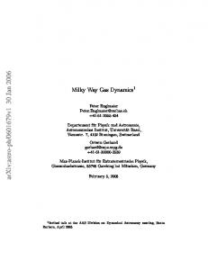
where Ω is a constant. Integrating (4.4) yields the solution u ¯®L Ω} (1, 0, 0)u (4.25) ! ! for the velocity field. The vorticity vector of the field from (4.5) has the form ω ¯ ¡¬u ¯ L r¡} r(0, 0, Ω). (4.26) ! By choosing f(} ) ¯ L } in Boillat’s simple-wave solution ansatz (4.3), for the " wave phase } we obtain ya , ya ¯ y®u y t, (4.27) ! L " where u y is the y component of u . From (4.24) and (4.25), ! ! L Ωya L Ω ex, u ¯® ! ω ¯ ! ez, (4.28) L L " " are the solutions for u and ω. This solution corresponds to a simple shear flow in which u ¯ ux(y, t)ex varies linearly with y, and which reverses direction as ya changes sign. This flow is depicted schematically in Fig. 1 (a). The left panel shows the variation of ux with ya , whereas the right panel shows the vorticity ω as a function of ya . Figures 1 (b, c) show further examples of shear flows that correspond to different choices of f(} ). In Fig. 1 (b), }¯

0Lya"1 ,

} ¯ tan−" whereas in Fig. 1 (c),

} ¯ sgn(ya )

f(} ) ¯ L tan } , "

(4.29)

0Lrya"r1"/#,

(4.30)

where sgn(ya ) denotes the sign of ya . In the solution (4.30), f(} ) ¯ } #L if ya " 0 and "

434

G. M. Webb et al.

1.0

1.2 1.0

0.5 0.8 ω

y 0

(a)

0.6 0.4

– 0.5 0.2 0 –1.0

– 0.5

0

0.5

0 –1.0

1.0

– 0.5

0

0.5

1.0

1.2 4 1.0 2

0.8 ω

y 0

0.6

–2

0.4

(b)

0.2 –4 –1

0

0 –1.0

1

1.0

– 0.5

0

0.5

1.0

10 8

0.5 ω

y

6

0

(c) 4

– 0.5

–1.0 –1.0

2

– 0.5

0 ux

0.5

1.0

0 –1.0

– 0.5

0 y

0.5

1.0

Figure 1. Examples of fluid velocity profiles u ¯ u(y)ex ¯®L Ω} ex (Ω ¯ const) and the ! vorticity ω ¯ ωez for the simple shear waves of (4.24)–(4.31), for which (a) } ¯ ya }L ; " (b) } ¯ tan−" (ya }L ) and (c) } ¯ ya }(L rya r)"/#, where ya ¯ y®u y t and } is the wave phase. " " !

f(} ) ¯ } #L if ya ! 0. Note that there is a possible ambiguity in the solution in " this case, depending on whether one chooses the positive or negative square root of rf(} )r. This last example shows that not all choices of f(} ) lead to analytic behaviour, because the vorticity ω¯ diverges at ya ¯ 0 in this case.

0 1

ΩL L "/# ! " e z 2L rya r "

(4.31)

435

Multidimensional simple waves in gas dynamics 4.2. Two-dimensional vortex flows The simple waves of interest are governed by (4.1)–(4.4), in which n(} ) ¯ (®sin } , cos } , 0),

Ω ¯ (0, 0, Ω(} ))

(4.32)

are the forms assumed for n(} ) and Ω(} ). These solutions turn out to be related to the two-dimensional vortex flows governed by (4.16)–(4.19), in which the streamfunction ψ(x, y, t) plays a central role. From (4.4) and (4.32), the fluid velocity u(} ) in these solutions is given by u(} ) ¯®L !

0&

}

}

Ω(} «) cos } «d} «, !

&

}

}

!

1

Ω(} «) sin } «d} «, 0 u , !

(4.33)

where u ¯ u at } ¯ } . ! ! Now consider the streamline equations (3.54) for the solution (4.33). Using the Frenet frame, in which the basis vectors ²e , e , e ´ framing the curve with " # $ tangent vector e 3 n(} ) are defined in (3.43), we obtain the streamline " equations in the form

0

where

1

0

1

¦q u u df du $ ¯® τκ $ q $ t " , # ¦} u u d} d} " " ¦q u u df du # ¯®τq ®κ # q # t " ®κ( fu t), $ " ¦} u # u d} d} " "

0

1

(4.34) (4.35)

e ¯ (®sin } , cos } , 0), e ¯ (®cos } , ®sin } , 0), e ¯ (0, 0, 1) (4.36) " # $ are the basis vectors for the Frenet frame. The curvature and torsion coefficients of the curve (3.36) with tangent vector e ¯ n(} ) are κ ¯ 1 and τ ¯ " 0. In this case, the curve (3.36) consists of the unit circle centred on X . In (4.34) ! and (4.35), q ¯ r[e ¯®x sin } y cos } , 5 " " q ¯ r[e ¯®x cos } ®y sin } , 67 (4.37) # # q ¯ r[e ¯ z, 8 $ $ The fluid velocity components in the Frenet frame may be written in the form

& u ¯L & # !

u ¯L " !

}

}

!

}

}

!

Ω(} «) sin (} ®} «) d} «u y cos } ®u x sin } , ! !

5

Ω(} «) cos (} ®} «) d} «®(u x cos } u y sin } ), ! !

6 7

(4.38)

u ¯ u z ¯ 0. 8 $ ! In (4.38) and in the following analysis, we restrict our attention to flows with u z ¯ 0. ! Taking into account that κ ¯ 1 and τ ¯ 0, the streamline equations (4.34) and (4.35) integrate to yield the solutions q ¯ z ¯ z ¯ const, $ ! 1 [u q ]}} ψ®L q ¯ # " ! ! # u "

0

(4.39)

&

}

}

!

Ω(} «) q (} «, t) d} « "

1

(4.40)

436

G. M. Webb et al.

for q and q , in which $ #

q ¯ f(} )tu (} ) (4.41) " " is the component of r parallel to e . The integration constant ψ in (4.40) may " be identified with the streamfunction ψ(x, y, t) for the flow. The form of the streamlines in terms of (x(} , t), y(} , t), z) may be obtained by inverting (4.37) to yield x ¯®q (} , t) sin } ®q (} , t) cos } , 5 " # (4.42) y ¯ q (} , t) cos } ®q (} , t) sin } , 67 " # z¯z , 8 ! where q and q are given by (4.39)–(4.41). " # A discussion of the streamline equations (4.39)–(4.42) from the perspective of the Hamiltonian streamline formulation of Sec. 3.2.1 is given in Appendix C. In Appendix C we also show that the streamfunction ψ in (4.40) satisfies the vorticity-advection equation (4.15). Example 1. A simple example of a two-dimensional (2D) vortex simple wave is obtained by considering the case where n ¯ (®sin } , cos } , 0),

Ω ¯ (0, 0, Ω ), !

and Ω is a constant. By choosing ! u y ¯ L Ω cos } , u x ¯®L Ω sin } , ! ! ! ! ! ! ! ! (4.33) and (4.38) yield the results

u z ¯ 0, !

(4.43)

(4.44)

uy ¯ L Ω cos } , uz ¯ 0, 5 ux ¯®L Ω sin } , ! ! ! ! 6 (4.45) 7 u ¯ L Ω , u ¯ 0, u ¯ 0, 8 " ! ! # $ for the velocity components in rectangular Cartesian coordinates, and in the Frenet frame. Consider the case of a centred simple wave in which f(} ) ¯ 0. Boillat’s ansatz for the wave phase may be written as ®x sin } y cos } ®L Ω t ¯ 0. (4.46) ! ! Alternatively, using cylindrical polar coordinates (r, θ, z), (4.46) for the wave phase } may be written as Because

r sin (θ®} )®L Ω t ¯ 0. ! !

F ¯ r cos (θ®} ) ¯ [r#®(L Ω t)#]"/# ! ! must be positive, it follows that } ¯ θ®sin−"

0L! rΩ! t1

(4.47) (4.48)

(4.49)

is the required solution for } (modulo 2π). Equation (4.48) shows that the solution of interest is restricted to the region r " rcrit ¯ L Ω t. ! !

(4.50)

437

Multidimensional simple waves in gas dynamics From (4.5), the vorticity of the flow is given by L Ω ! ! e, [r#®(L Ω t)#]"/# z ! ! and hence the vorticity diverges at r ¯ rcrit. Equations (4.39)–(4.41) now yield the solutions ω¯

(4.51)

ψ q ¯ ®tL Ω (} ®} ), q ¯z¯z (4.52) # L Ω ! ! ! $ ! ! ! for the fluid-velocity streamlines, where the streamfunction ψ is constant on the streamlines. Using the transformations (4.42) and (4.52), the streamline equations for (x, y, z) reduce to q ¯ tL Ω , " ! !

9

:

ψ x ¯®tL Ω sin } ® ®tL Ω (} ®} ) cos } , ! ! ! ! ! L Ωο !

9

5

:

6 (4.53) ψ 7 y ¯ tL Ω cos } ® ®tL Ω (} ®} ) sin } , ! ! ! ! ! L Ω ! ! z¯z . 8 ! Note that } plays the role of the parameter along the streamline. In order that F 3®q be positive, it is necessary to choose } " } ψ}(L# Ω# t) in the ! ! # ! streamline equations (4.53). From (4.52),

ψ ¯ L Ω ²tL Ω (} ®} )®[r#®(L Ω t)#]"/#´ ! ! ! ! ! ! ! L Ω t 3 L Ω tL Ω θ®sin−" ! ! ®} ®[r#®(L Ω t)#]"/# ! ! ! ! ! ! ! r

(

9

0

1 :

*

(4.54)

is the streamfunction ψ(r, θ, t) for the vortex simple-wave solution. Figure 2 shows the vortex simple-wave streamline (4.53) for the parameter values L Ω ¯ 1, } ¯ 0 and t ¯ 1, where we choose } & ψ}t to ensure that ! ! ! F & 0. The streamlines (the solid lines) consist of spirals in the (x, y) plane that are radial at the innermost radius r ¯ rcrit ¯ L Ω t and become azimuthal as ! ! r U¢. The solution (4.53) only applies for r & rcrit. The vorticity ω for the solution diverges at r ¯ rcrit, and ω C L Ω }r as r U¢. Also shown in Fig. 2 are ! ! examples of constant-phase fronts for the simple wave (the straight dashed lines). The envelope of the family of plane-wave fronts obtained by varying } is the circle r ¯ rcrit. This circle is the group-velocity surface r ¯ ut, where u ¯ L Ω (®sin } , cos } , 0) is the group velocity. ! ! Burnat (1971) presented a solution of the magnetohydrodynamic equations in which the streamlines and the magnetic field lines are identical and consist of spirals similar to those depicted in Fig. 2. Burnat’s solutions, like those in Fig. 2, have unbounded derivatives on the wave envelope. Using the solution (4.12), or integrating (4.11), yields r ¯ (r#L# Ω# t#)"/#, ! ! !

0L!rΩ! ! t1

θ ¯ θ tan−" !

(4.55)

438

G. M. Webb et al. 4

2

y 0

–2

–4 –4

–2

0 x

2

4

Figure 2. Streamlines for the time-dependent 2D simple vortex wave described by (4.43)–(4.46), in which Ω ¯ Ω ez is a constant vector along the z axis and n ¯ (®sin } , cos ! } , 0) is the wave normal. The outward spiral flow lines (4.53) are restricted to the (x, y) plane. The dashed straight lines are representative constant phase fronts (i.e. } ¯ const). The envelope of the family of phase fronts is given by the circle. The vorticity and fluid gradients diverge on the wave envelope.

for the fluid-particle paths, where r ¯ r and θ ¯ θ at t ¯ 0. Solving (4.55) for ! ! r and θ yields the equations ! ! L Ω t ! ! r ¯ (r#®L# Ω# t#)"/#, . (4.56) θ ¯ θ®tan−" ! ! ! ! (r#®L# Ω# t#)"/# ! ! From (4.56), one can show that θ 3 } (r, θ, t) is the simple-wave phase (4.49). It ! is of interest to note that the vorticity for the simple vortex wave, ω ¯ L Ω }r , ! ! ! is a function of the Lagrangian variable r . Hence, both ω and } 3 θ are ! ! Lagrangian variables. The streamfunction ψ in (4.54) may be written in the form ψ ¯ L Ω [L Ω tθ (r, θ, t)®r (r, t)], (4.57) ! ! ! ! ! ! where we have set } ¯ 0 in (4.54). This shows that the streamfunction is most ! naturally expressed in terms of the Lagrangian variables θ and r . The fluid! ! particle paths (4.12) consist of straight lines in the (x, y) plane. The fluid velocity u ¯ L Ω n in this example is normal to the wave fronts. One can ! ! construct the streamlines at time t from the streamlines at time t by displacing # " the wave fronts a distance L Ω (t ®t ) normal to the front. Equation (4.57) for ! ! # " ψ shows that ψ ¯ ψ (L Ω )#θ (t ®t ) is the change of ψ induced by following # " ! ! ! # " the particle paths. The fluid velocity for the vortex simple wave may be written in the form

9

:

u ¯ L Ω r ¡θ ¯ L Ω n. (4.58) ! ! ! ! ! ! The result (4.58) for u in terms of r and θ shows that r and θ are Clebsch ! ! ! ! variables for the solution (see e.g. Holm and Kuperschmidt 1983 ; Zakharov and


439

Kuznetsov 1984). The relationship between the advection equation for r and ! θ and the Hamiltonian Poisson bracket (4.22) is considered in Appendix D. It ! is straightforward to generalize the above solution to the case where u z 1 0, ! when one obtains helical-spiral-type streamlines for the flow. Example. 2. As a second example of a vortex simple wave, consider a solution of the form (4.33) for u(} ) in which the angular velocity Ω ¯ Ω(} )ez is not constant. In particular, the choice n ¯ e ¯ (®sin } , cos } , 0) (4.59) Ω ¯ (} c®} )e , $ " leads to the solution (4.60) u(} ) ¯ (} c®} )e ®e " # for the fluid velocity, where the orthonormal triad ²e , e , e ´ is defined in (4.36), " # $ } c is a constant, and dimensionless variables have been adopted. We consider the case of a centred simple wave in which f(} ) ¯ 0. Boillat’s ansatz (4.3) for the wave phase } reduces to G 3 x sin } ®y cos } (} c®} )t ¯ (} c®} )t®r sin (θ®} ) ¯ 0.

(4.61)

Thus, in polar coordinates (r, θ, z), the wave-front equations are

9(} c®}r )t: ,

θ ¯ } sin−"

z ¯ z ¯ constant. !

(4.62)

It is of interest to note that the curve X* ¯ u(} ) in (4.60) is the involute of the circle X ¯ (cos } , sin } , 0) (see Lipschutz 1969). Equations (4.34)–(4.37) integrate to yield the streamlines x ¯®q sin } ®q cos } , " # where

y ¯ q cos } ®q sin } , " #

z¯z , !

(4.63)

5 q ¯ r sin (θ®} ) ¯ (} c®} )t, " t["(} ®} c)$®} ]®ψ 67 q ¯®r cos (θ®} ) ¯ $ . # } ®} c 8

(4.64)

[(} c®} )%t#²t["(} ®} c)$®} ]®ψ´#]"/# $ r} ®} cr

(4.65)

The equation r¯

and (4.62) give the streamlines in polar coordinates. The integration constant ψ in the streamline equations (4.64) is the streamfunction for the solution, so that u ¯ ¡ψ¬ez is the fluid velocity (4.60) for the simple wave. The simple wave is restricted to regions where F 3 1}r¡} r, (4.6), is positive. In the present example, (4.66) F ¯®q ®t ¯ x cos } y sin ®t ¯ r cos (θ®} )®t. # The envelope of the family of phase fronts (4.61), satisfying the equations G(} , r, t) ¯ 0 and G} 3 F ¯ 0, yields the group-velocity surface r ¯ u(} )t of the simple wave. Note, however, that the envelope of the family of phase fronts for a non-centred wave in which f(} ) 1 0 does not in general coincide with the group-velocity surface. There are two possible solution branches for the

440

G. M. Webb et al.

envelope, obtained by eliminating } between (4.62) and the equation F ¯ 0. If 0 ! θ®} ! "π, the envelope may be written as # 5 t (r#®t#)"/# θ ¯ θ−b 3 } ccos−" ® , r t 6 (4.67) 7 (r#®t#)"/# , } ¯ } −b 3 } c® t 8

01

whereas if ®"π ! θ®} ! 0, the envelope is described by # 5 (r#®t#)"/# t θ ¯ θ+b 3 } c , ®cos−" r t

01

(4.68) 6

(r#®t#)"/#

} ¯ } +b 3 } c

t

7

. 8

It is straightforward to show that θ+b " θ−b for the wave envelope boundaries

(4.67) and (4.68). Note that r " t is required for the envelopes to be well defined. Since } may be used as a parameter along the streamlines, it is of interest to know the behaviour of F as a function of } on the streamline. From (4.64) and (4.66), t[} ®"(} ®} c)$]ψ , (4.69) F¯ c $ } ®} c on the streamline ψ ¯ const. Alternatively, F may be expressed in the form F¯ where

t(} b®} ) ²[} ®} c"(} b®} c)]#$(} b®} c)#´, # % 3(} ®} c) } b ¯ } c[3(} cψ}t)]"/$.

(4.70) (4.71)

Equations (4.70) and (4.71) show that there are two cases of interest in which F & 0, namely } c ! } ! } +b : } −b ! } ! } c :

} +b ¯ } c[3(} cψ}t)]"/$, } −b ¯ } c®(3r} cψ}tr)"/$,

5

(4.72) 7

6

8

where } cψ}t " 0 for the } +b branch, and } cψ}t ! 0 for the } −b branch. , Equation (4.65) shows that r U¢ along the streamline as } U } c. As } U } ³ b F U 0 and the streamline meets the envelope curves (4.67) and (4.68) respectively. Figures 3 and 4 illustrate the streamlines (4.63) for the simple wave for the case } c ¯ "π at time t ¯ 1. The example in Fig. 3 corresponds to the θ−b branch # solution for the wave envelope. The streamlines are the solid curves, while the dashed curve represents the wave envelope. The streamlines are restricted to the region r " rb(θ, t), where rb denotes the wave-envelope boundary. The straight-line tangents to the envelope represent wave fronts on which } is constant. Note that the wave envelope meets the circle r ¯ t as } U } c ¯ "π and # θ U "π. The streamline for ψ U®t} c corresponds to the straight-line segment # y & t along the y axis. The streamline representation in terms of } is problematical for ψ ¯®t} c, since } b ¯ } c in this case. The range of θ has been restricted


441

15

10

5

y 0

–5

– 10

–15 –15

– 10

–5

0 x

5

10

15

Figure 3. Streamlines for the time-dependent 2D simple vortex wave described by (4.59)–(4.61), for which Ω ¯ (} c®} )ez and n ¯ (®sin } , cos } , 0). The streamlines are restricted to the region outside the wave envelope (the dashed spiral). The parameter } c ¯ "π and γ ¯ &. # $ 15

10

5

y 0

–5

– 10

–15 –15

– 10

–5

0 x

5

10

15

Figure 4. Same as Fig. 3, except that the sense of rotation of the envelope and fluid streamlines is reversed.

to the range ®$π ! θ ! "π in Fig. 3 to ensure a single-valued solution for the # # streamfunction. Figure 4 shows a similar plot of the streamlines for the θ+b solution for } c ¯ "π. The solution in Fig. 4 is similar to that in Fig. 3, except that # the sense of rotation of the spirals is opposite to that in Fig. 3. One can show

442

G. M. Webb et al. 15

10

5

y 0

–5

– 10

–15 –15

– 10

–5

5

0 x

10

15

Figure 5. The wave envelope of Figure 4, for a case where the range of θ has not been truncated to ensure a single-valued solution.

that as } U } c and r U¢, the streamlines in both figures become parallel to the y axis. Figure 5 illustrates the wave-envelope boundary θ ¯ θ+b for a case where the range of θ has not been truncated to ensure a single-valued streamfunction ψ. The Lagrangian particle paths (4.12) in cylindrical polar coordinates are r ¯ [(r t)#(θ ®} c)#t#]"/#, ! !

θ ¯ θ sin−" !

9(} c®θr !)t: ,

(4.73)

where θc 3 } and r 3 F are the Lagrangian variables. The fluid velocity (4.60) ! admits the Clebsch representation µ ¯ "(} ®} c)#. (4.74) # It is possible to relate the advection equations for } and F to the Hamiltonian formulation (4.20)–(4.22) in a way similar to that in Appendix D for the first example. One can also develop a Clebsch representation for u using the rectangular Cartesian coordinates x ¯ F cos } and y ¯ F sin } representing the ! ! initial fluid-particle position. u ¯®(F®t)¡µ¡F,

5. Simple sound waves In this section, we consider simple sound waves. The eigenequations (3.20) for the sound waves reduce to du ρ« ¯ c n(} ), d} ρ where

dS ¯ 0, d}

λ ¯ u[n(} )c

(5.1) (5.2)


443

is the characteristic speed of the phase front. Without loss of generality, we have chosen the ‘ forward ’ sound-wave eigenmode. Because u ¯ u(} ), we obtain ω ¯ ¡¬u ¯ c

ρ« n¬¡} ¯ 0 ρ

(5.3)

for the fluid vorticity, where n ¯ ¡} }r¡} r is the normal to the wave front. Similarly, d cρ« 1 d cρ« ¡[u ¯ r¡} r 3 . (5.4) d} ρ F d} ρ

0 1

0 1

The remaining equation needed to determine the simple sound wave is Boillat’s equation (3.25) for the wave phase } : G 3 f(} )λ(} )t®r[n(} ) ¯ 0.

(5.5)

The group velocity for the wave from (3.28) is Vg ¯ ucn. Equations (5.1) may be integrated to yield u¯

&

}

}

c !

ρ« n(} *) d} *u , ! ρ

ρ ¯ ρ(} ),

S¯S !

(5.6)

for the velocity u and entropy S, where u and S are integration constants. ! ! Equations (5.1)–(5.6) show that simple sound waves are compressible, irrotational isentropic flows. Since ¡¬u ¯ 0, u ¯ ¡Φ, where Φ is the velocity potential. By using the Frenet frame, one can show that the velocity potential Φ has the form } ρ« (5.7) Φ ¯ r[u® d} q c g(t), " ρ } ! where q ¯ r[n ¯ f(} )λ(} )t (5.8) " (see Appendix E) and g(t) is a linear function of t determined below. The fluid equations for irrotational, compressible isentropic flows may be reduced to the mass-continuity equation and Bernoulli’s equation,

&

¦ρ ¡[( ρ¡Φ) ¯ 0, ¦t

¦Φ "r¡Φr#W ¯ 0, ¦t #

(5.9)

for ρ and Φ, where W( ρ) is the gas enthalpy (W ¯ γp}[(γ®1)ρ] ¯ c#}(γ®1 for an adiabatic gas). In order to satisfy Bernoulli’s equation, the function g(t) in (5.7) must be of the form (5.10) g(t) ¯®("rur#W) tk , # ! " where the subscript 0 denotes evaluation at } ¯ } , and k is an arbitrary ! " constant. Equations (5.9) may be written in the Hamiltonian form (see e.g. Zakharov and Kuznetsov 1984) ¦ρ δH ¯ , ¦t δΦ

¦Φ δH ¯® , ¦t δρ

(5.11)

H ¯ ["ρr¡Φr#ε( ρ)] d$x #

(5.12)

where the Hamiltonian functional

&

444

G. M. Webb et al.

consists of the kinetic plus internal energy of the gas. For an adiabatic gas, the internal energy density ε ¯ p}(γ®1). Thus the velocity potential in (5.7) plays a central role in the Hamiltonian formulation of simple sound waves. In Sec. 5.1, we discuss time-dependent simple waves in one Cartesian space dimension, in which n ¯ (1, 0, 0) is a constant vector along the x axis. Although this solution has been discussed extensively in standard texts (e.g. Whitham 1974 ; Courant and Friedrichs 1976 ; Landau and Lifshitz 1987), our main aim is to show the central role of the envelope of the family of wave fronts in the (x, t) plane for wave breaking. In Sec. 5.2, we present an explicit example of a two-dimensional simple sound wave, where the basic properties of the solution depend critically on the envelope of the family of wave fronts. Unlike the onedimensional simple sound wave, the 2D sound wave has unbounded derivatives at all times t " 0 on the envelope. In Sec. 5.3, we make some brief comments on time-independent simple waves in two Cartesian space dimensions and discuss the role of Boillat’s ansatz (5.5) for the wave phase in this case. 5.1. One-dimensional simple sound waves For n ¯ (1, 0, 0), (5.1) integrates to yield the solution u ¯ R−

&

ρ

ρ

!

c 2 dρ 3 u (c®c ), ! ! ρ γ®1

(5.13)

and S ¯ S ¯ const for the one-dimensional simple sound wave, where uex is the ! fluid velocity along the x axis. In (5.13),

01

ρ 0γ−")/# (5.14) c¯c ! ρ ! is the gas sound speed for a polytropic equation of state p ¯ p ( ρ}ρ )γ, and ! ! c ¯ (γp }ρ )"/# is the sound speed for ρ ¯ ρ . Choosing f(} ) ¯ } in (5.5), the ! ! ! ! equation for the wave phase reduces to } ¯ x®λ+(} )t,

λ+ ¯ uc,

(5.15)

corresponding to the forward sound wave. The constant of integration R− in (5.13) may be identified as the Riemann invariant for the backward sound wave, i.e. R− is constant on the backward sound-wave characteristic : ¦R− ¦R− (u®c) ¯ 0. ¦t ¦x

(5.16)

To obtain the simple-wave solution, one specifies the initial density profile at time t ¯ 0 : (5.17) ρ(x, 0) ¯ ρi(x). The solution for ρ at time t is ρ ¯ ρi(} ). The solution for c is given by (5.14), and (5.13) gives the solution for u. A straightforward calculation shows that ρx ¯

dρ}d} , F

ρt ¯®λ+

dρ}d} , F

(5.18)


445

where F 3 G} ¯ 1t

dλ+ , d}

G ¯ } λ+ t®x ¯ 0.

(5.19)

Thus, at points where F 1 0, ρ and u satisfy the forward sound-wave equation ¦ρ ¦ρ (uc) ¯ 0, ¦t ¦x

(5.20)

and a similar equation applies for the evolution of u. The derivatives ρx and ρt diverge on the phase-front envelope G ¯ G} ¯ 0. Thus, the wave breaks when F ¯ G} ¯ 0 at time t ¯ tB, where 1 . tB ¯® dλ+}d}

(5.21)

The time tB " 0 if dλ+}d} ! 0. As an example of wave breaking, consider the initial conditions

0 1

x# ρ(x, 0) ¯ ρi(x) ¯ ρ exp ® ! L#

(5.22)

for the density profile. In this case, the wave breaks at time tB ¯

L# . (γ1) } c(} )

(5.23)

From (5.19) and (5.23), one finds that the minimum value of tB occurs when } ¯ L}(γ®1)"/#, and the value of x at the minimum break time follows from (5.15). The above analysis indicates that the envelope of the family of phase fronts G ¯ G} ¯ 0 plays a central role in the evolution of the one-dimensional simple sound wave. The envelope consists of a curve in the (x, t) plane. From the envelope, it is straightforward to generate the family of phase fronts by drawing straight-line tangents x ¯ λ+(} )t} to the envelope for each fixed value of } . The envelope of the family of phase fronts also plays a central role in the 2D simple sound waves considered in the next section. 5.2. Multidimensional simple sound waves In the general multidimensional case, the eigenequations (5.1) have solutions of the form (5.6). Consider a two-dimensional simple sound wave in which the wave normal n(} ) 3 e corresponds to the tangent vector to a space curve x ¯ " X(} ), and for which the Frenet frame for the curve consists of the orthonormal triad ²e , e , e ´ defined by the equations " # $ n 3 e ¯ (®sin } , cos } , 0), e ¯ (®cos } , ®sin } , 0), e ¯ (0, 0, 1). (5.24) " # $ The curvature and torsion coefficients for the curve are κ ¯ 1 and τ ¯ 0 (i.e. X(} ) is a circle). Choosing the functional forms ρ ¯ ρ (cos# } )α, !

01

ρ (γ−")/# , c¯c ! ρ !

α¯

2 γ®1

(5.25)

446

G. M. Webb et al.

yields solutions (5.6) for u of the form ux ¯ ux #αco(sin$ } ®sin$ } ), 5 ! $ ! 67 (5.26) uy ¯ uy #αc (cos$ } ®cos$ } ). 8 ! ! $ ! For the sake of simplicity, we further restrict our attention to the case uy ¯ #αc cos$ } (5.27) ux ¯ #αc sin$ } , $ ! $ ! by appropriate choice of u and } in (5.26). From (5.25), the sound speed in the ! ! model varies as c ¯ c cos# } . (5.28) ! For the case of an adiabatic gas with adiabatic index γ ¯ & and α ¯ 3, and the $ gas is supersonic throughout the flow (rur#®c# " 0). By appropriate choice of u ! and } in (5.26), one can obtain both subsonic and supersonic flows. ! The components of the fluid velocity relative to the Frenet frame (5.24) are and

u ¯ #αc cos (2} ), " $ !

u ¯®"α c sin (2} ), # $ !

u ¯ 0, $

(5.29)

λ ¯ u c ¯ "c (Λ cos 2} 1), Λ ¯ "(4α3), (5.30) " #! $ is the phase speed of the wave. Note Λ ¯ 5 if γ ¯ & and α ¯ 3. $ We consider the case of a centred simple wave, for which Boillat’s phase ansatz (5.5) reduces to G 3 λ(} )t®(®x sin } y cos } ) ¯ 0.

(5.31)

The envelope of the family of plane-wave fronts obtained by varying } in (5.31) yields the equations G ¯ λ(} )t®q ¯ 0, "

G} 3 F ¯ t

dλ ®q ¯ 0 # d}

(5.32)

for the envelope, where q ¯®x sin } y cos } , q ¯®x cos } ®y sin } (5.33) " # are the position-vector components q ¯ r[e and q ¯ r[e relative to the " " # # Frenet frame base (5.24). By inverting (5.33) it follows that the envelope of the family of plane-wave fronts (5.32) is given by the equations where

x(} ) ¯®q sin } ®q cos } , " #

y(} ) ¯ q cos } ®q sin } , " #

q ¯®c Λt sin 2} . q ¯ λ(} )t ¯ "c t(Λ cos 2} 1), #! # ! " The non-normalized tangent vector to the envelope (5.34) is given by T¯

0d}dx , d}dy , d}dz 1 ¯ t0d}d#λ#λ1 e# ¯ "#c! t(1®3Λ cos 2} )e#.

(5.34) (5.35)

(5.36)

From (5.36), the tangent vector T vanishes when

9

0 1:

1 1 } ¯ } c ¯ 2nπ³cos−" , 2 3Λ where n is an integer.

(5.37)


447

4

2

y 0

–2

–4 –4

–2

0 x

2

4

Figure 6. The envelope (5.34), (5.35) of the family of phase fronts (5.31) for the simple soundwave solution described by (5.24)–(5.31). The cusps in the envelope occur when } has the values (5.38). The time t ¯ 1, γ ¯ & and } c ¯ 43.089°. $ "

The form of the envelope (5.34), (5.35) in the (x, y) plane obtained by varying the parameter } at time t ¯ 1 and with γ ¯ & is displayed in Fig. 6. The envelope $ consists of a four-cornered, distorted rectangle with cusped corners where the tangent vector (5.36) vanishes. The cusps occur at

0 1

1 } ¯ } c ¯ cos−" , " 3Λ

} c ¯ π®} c , # "

} c ¯ π} c , $ "

} c ¯ 2π®} c . % " (5.38)

The point on the envelope where x ¯ 0 and y " 0 corresponds to } ¯ 0. At the cusp in the first quadrant (x " 0, y " 0), } ¯ } c ¯ 43.089°, and } increases in a " clockwise fashion as one proceeds around the envelope. Figures 7 (a, b) illustrate the possible wave phase fronts associated with a fixed field point P. In Fig. 7 (a), the P is outside the wave envelope, whereas P lies inside the wave envelope in Fig. 7 (b). The wave fronts consist of the straight-line tangents (5.31) to the wave phase envelope. In Fig. 7 (a), there are apparently two possible tangents to points on the wave envelope corresponding to a fixed point P outside the envelope. However, it turns out that only the tangent QP is applicable, because we require that F ¯ 1}r¡} r 3 G} be positive in (3.26) at points off the envelope. Consider, for example, the tangent QP in Fig. 7 (a), in which Q has coordinates (x , y ) and for ! ! which } ¯ } . The general point (x, y) on the straight-line tangent satisfies the ! equation λ(} )tx sin } ®y cos } ¯ 0, (5.39) ! ! ! and, in particular, the point (x , y ) satisfies (5.39). As a consequence, the ! ! equation of the tangent (5.39) may be expressed in the form (x®x ) sin } ®(y®y ) cos } ¯ 0. ! ! ! !

(5.40)

448

G. M. Webb et al.

6

6 (a) 4

4

(b)

Q 2

2

P

P y 0

y 0

–2

–2

–4 –6 –6

–4

R

–4

–2

0 x

2

4

6

–6 –6

–4

–2

0 x

2

4

6

Figure 7. Constant phase fronts that are tangent to the wave envelope (5.34), (5.35) for the simple sound wave (5.24)–(5.31). In (a), there are two possible tangents to the wave envelope passing through a point P located outside the envelope. In (b), the point P is located inside the envelope. For points P inside the envelope, up to four tangents may be drawn. The values of } associated with each tangent are possible for } at point P.

On the tangent QP, F 3 G} ¯ t

0d}dλ1!x cos } !y sin } !.

(5.41)

Because F 3 F (x , y , } , t) ¯ 0 on the wave envelope, (5.40) and (5.41) yield ! ! ! ! the results F 3 F®F ¯ (x®x ) cos } (y®y ) sin } ! ! ! ! ! x®x y®y !¯ ! (5.42) ¯ cos } sin } ! ! at any point P(x, y) on the tangent QP. It follows from the results (5.42) that if cos } " 0 and x " x or if cos } ! 0 and x ! x then F " 0. Similarly, if ! ! ! ! (y®y ) sin } " 0 then F " 0. For the point P in Fig. 7 (a), only the tangent QP ! ! has F " 0, whereas F ! 0 for the tangent RP. Thus, for points outside the wave envelope, the solution of (5.39) for } 3 } is unique, since we require F " 0. ! Hence the flow is single-valued and the physical variables are continuous and differentiable outside the wave envelope. The derivatives of } and the physical variables become unbounded on the wave envelope owing to a jump in the value of } on the envelope. A similar argument applied to points P inside the wave envelope (as illustrated in Fig. 7 b), does not lead to a unique solution for } inside the wave envelope, unless one or more sides of the envelope are deleted. Now consider the character of the fluid streamlines (3.34) in the region outside the envelope. In terms of q , q and q , the streamline equations (3.54) " # $ reduce to dq u u dq # # q ¯ # q! ®q , $¯0 (5.43) d} u # u " " d} " "

449

Multidimensional simple waves in gas dynamics 10

5

y 0

–5

– 10 – 10

–5

0 x

5

10

Figure 8. The streamlines (5.48) at time t ¯ 0 for the simple sound wave (5.24)–(5.31). The straight-line separatrices at 45° correspond to the constant-phase fronts } ¯ "π, $π, &π and (π. % % % %

in the present example. Using the results (5.30) and noting that q ¯ λ(} )t, " (5.43) may be integrated to yield the solutions

9

where

1 q ¯ q! cs®"c t #! # " I # q 3 z ¯ z ¯ const, $ !

&

}

}

s

:

5

I (} «) (1®3Λ cos 2} «) d} « , # 6

(5.44) 7

8

(5.45) I (} ) ¯ r cos 2} r"/%, q ¯ "c t(Λ cos 2} 1). # " #! The function I (} ) is the integrating factor for (5.43), and cs is related to } s by # the equation (5.46) cs ¯ I (} ) [q (} , t)®q!t(} , t)]r} =} , # # s and } ¯ } s corresponds to a fixed point on the streamline. The streamlines x ¯ X(} , t) and y ¯ Y(} , t) now follow from the transformations (5.34) between (q , q ) and (x, y). The wave phase } plays the role of a parameter along the " # streamlines. At time t ¯ 0, the streamline solutions (5.44)–(5.46) reduce to c cs ¯ q s I s, (5.47) q ¯ s, # # # I # where the subscript s denotes that } ¯ } s. In terms of x and y, the streamlines at time t ¯ 0 have the forms q ¯ 0, "

cos } sin } , y ¯®q s I s . (5.48) x ¯®q s I s # # I (} ) # # I (} ) # # Figure 8 illustrates the streamlines (5.48) at time t ¯ 0. The flow consists of four

450

G. M. Webb et al.

flows separated by the straight-line wave fronts : } ¯ "π, $π, &π and (π. The % % % % phase fronts for } ¯ "π, $π, &π and (π are also streamlines, but are not described % % % % by (5.48), since cos 2} ¯ 0 in these cases. The form of the streamlines at time t ¯ 1 is illustrated in Fig. 9 The flow separates into four distinct regions corresponding to the top, left-hand side, bottom and right-hand side of the wave envelope. Some of the incoming streamlines from infinity impinge on the wave envelope. For this simple wave flow to be used in a physical application would require matching the flow to another solution of the fluid equations before the flow hits the wave envelope. The flow near the cusps either flows inward toward the cusps or diverges to infinity. From (5.44) and (5.45), rq r U¢ as } U "π, $π and (π. The solution (5.44) % % % # for q does not apply for } an odd multiple of "π. For } ¯ "π, $π, &π and (π, the % % % % % # streamlines coincide with the straight-line wave fronts, and correspond to flows emanating or diverging from near the cusps in Figs 6 and 9. Thus, for example, for } ¯ "π, the streamline equations % dx dy ¯ (5.49) ux uy have solutions c y ¯ x ! t, (5.50) 2"/# and similar results hold for } ¯ $π, &π and (π. As time increases, the wave % % % envelope and flow pattern move outward in such a way that the pattern is preserved. 5.3. Steady, simple sound waves In this section, we discuss steady, two-dimensional (2D) simple sound waves treated in standard texts (e.g. Courant and Friedrichs 1976, Chap. 4) from the perspective of Boillat’s simple-wave formalism. For time-independent simple waves, λ ¯®} t}r¡} r ¯ 0. Hence the eigenvalue equations for simple sound waves reduce to u[n³c ¯ 0,

(5.51)

and du ρ« ¯³c n, d} ρ

dS ¯0 d}

(5.52)

are the eigenvector relations. Because n ¯ ¡} }r¡} r, the eigenvalue equations (5.51) for 2D sound waves may be written in the form H ¯ (u#®c#)} #x2uv} x } y(v#®c#)} #y ¯ 0,

(5.53)

where the fluid velocity u ¯ uexvey and c are functions of } only. Since u ¯ u(} ) and v ¯ v(} ), J ¯ ¦(u, v)}¦(x, y) ¯ 0. The vanishing Jacobian condition J ¯ 0 indicates that the hodograph transformation is singular for simple waves. The characteristics of the partial differential equation (5.53), dx dy d} ¯ ¯ , 2[(u#®c#)} xuv} y] 2[(v#®c#)} yuv} x] 2Η

(5.54)


451

10

5

y 0

–5

– 10 – 10

–5

5

0 x

10

Figure 9. The streamlines and wave envelope at time t ¯ 1 for the simple sound-wave solution of (5.24)–(5.31).

imply that } is constant on the characteristics. Equations (5.54) lead to the equations dy (v#®c#)} yuv} x dy } ¯ ¯® x . , (5.55) dx (u#®c#)} xuv} y dx }y From (5.55), y« ¯ dy}dx satisfies the quadratic equation (y«)#(u#®c#)®2uvy«v#®c# ¯ 0,

(5.56)

with solutions y« ¯ ζ³ ¯

uv³c(u#v#®c#)"/# u#®c#

(5.57)

for y«. The eigenequations (5.52) for du}d} may be written in the form du ρ«} x , ¯c d} ρr¡} r

dv ρ«} y . ¯c d} ρr¡} r

(5.58)

Equations (5.58) imply that du } x ¯ ¯®y«. dv } y

(5.59)

Substitution of the result (5.59) for y« into (5.56) yields the characteristics in the (u, v) hodograph plane in the form (u duv dv)#®c#(du#dv#) ¯ 0, with integrals

&

θ³ (M#®1)"/#

dq ¯ Γ³, q

(5.60) (5.61)

452

G. M. Webb et al.

where q and θ are polar coordinates for u and v : u ¯ q cos θ,

v ¯ q sin θ,

q# ¯ u#v#,

M# ¯

q# , c#

(5.62)

and M is the sonic Mach number. The above development shows how Boillat’s formalism yields the characteristics for steady 2D simple sound waves in two Cartesian space coordinates x and y. The eigenvalue equation (5.51) was interpreted as a first-order partial differential equation for } , with characteristics (5.57) in the (x, y) plane. The characteristics in the (u, v) hodograph plane follow from the eigenvector relations (5.52).

6. Summary and discussion In this paper, we have studied some of the ramifications of Boillat’s (1970) formulation of multidimensional simple waves for hyperbolic systems of equations of type (3.1). The phase ansatz (3.25) derived by Boillat consists of planar wave fronts for constant wave phase } , which move with constant phase speed λ(} ) along the normal n(} ) to the front. The ansatz (3.25) for } (x, y, z, t) implicitly determines the wave phase for a given wave normal n(} ) and wave mode, and in which the arbitrary function f(} ) determines whether the wave is a centred or non-centred wave. The envelope of the family of phase fronts obtained by varying the wave phase } plays a central role in the solution examples for vortex simple waves (Sec. 4) and simple sound waves (Sec. 5). On the envelope, the gradients of } and the physical variables diverge. The phase fronts can readily be reconstructed once the envelope is specified. Perhaps the prototypical example of wave breaking, shock formation and gradient ‘ blow-up ’ is that for the inviscid Burgers equation, or that for timedependent simple sound waves in one Cartesian space dimension (see e.g. Whitham 1974). For appropriate initial conditions, the gradients blow up in a finite time t ¯ tB. If one considers the time t and space coordinate x to be complex variables, the singularity formation at time t ¯ tB corresponds to the instant when the singularity in the complex time domain first hits the real time axis (Caflisch et al. 1993). The break time t ¯ tB(x) corresponds to the envelope of the family of phase fronts (or characteristics) in the (x, t) plane. For time-dependent simple waves in two or more space dimensions, the examples of simple vortex waves (Sec. 4) and sound waves (Sec. 5) exhibit singular behaviour on the wave envelope at all times t (where t is taken to be a real variable). The examples studied in the present paper have a singularity at the origin of the (x, y) plane at time t ¯ 0. As time increases, the envelope of the family of phase fronts expands away from the origin. If one extrapolates the solutions to t ! 0, then the wave envelope converges toward the origin as t increases. The envelope can consist of a closed curve in the (x, y) plane (see e.g. Figs 1 and 9) or an open curve (see e.g. Figs 3 and 4). For the simple sound wave in Fig. 9, the physical solution is not well defined inside the envelope where the solution is multivalued, indicating that the solution must be matched onto another solution of the fluid equations on some boundary outside the envelope. The singularities that form in two or more space dimensions are similar to


453

caustics in geometrical optics, or the singularities that occur in linear wave equations in two or more space dimensions, in which caustics occur on the envelope of the family of plane-wave fronts. In Boillat’s formulation of simple waves, one is free to specify the wave normal n(} ) ¯ (nx, ny, nz). One can regard n(} ) 3 e as the tangent vector to a " three-dimensional space curve x ¯ X(} ). The twisting and turning of the curve x ¯ X(} ) may be conveniently described in terms of an orthonormal triad of vectors ²e , e , e ´ attached to the curve. In general, the frame vectors ²ei´ rotate " # $ as one progresses along the curve according to the twist equations dei}d} ¯ κ¬ei, where κ ¯ 3i κi ei is the twist vector (see e.g. Bishop 1975 ; Goriely and Tabor 1996 ; see also (3.36) et seq.). The twist equations are a natural generalization of the Serret–Frenet equations of classical differential geometry. The twist equations play an important role in the theory of knots, and in particular of knotted vortices in fluid dynamics (see e.g. Moffatt 1969 ; Moffatt et al. 1992) and knotted magnetic field lines in magnetohydrodynamics (Berger and Field 1984 ; Moffatt and Ricca 1992). One intriguing question left unanswered by the present paper is : What are the properties of simple waves in which n(} ) ¯ X«(} )}rX«(} )r is the tangent vector to a knotted space curve x ¯ X(} ) ? The wave phase } turns out to be a natural parameter for the fluid streamlines and the vortex streamlines (Sec. 3.2). The streamlines for the simple waves reduce to two coupled first-order ordinary differential equations in the independent variable } and the dependent variables q ¯ r[e and q ¯ r[e . # # $ $ The equation q 3 r[e ¯ f(} )λ(} )t corresponds to Boillat’s ansatz (3.25) for " " } . The equations may be expressed in terms of Lagrangian and Hamiltonian variational principles. The coefficients and source terms in the equations depend on the detailed form of the fluid velocity u(} ), Boillat’s ansatz (3.25) for the wave phase, and the curvature and torsion coefficients of the curve x ¯ X(} ). In Sec. 3.3 we discussed the link between characteristic surfaces and simple waves (see e.g. Burnat 1965, 1971 ; Courant and Hilbert 1989). The simple-wave phase surfaces } ¯ const correspond to a special class of characteristic surfaces in which the fluid variables are solely functions of } . For more general solutions of the fluid equations, the physical variables will depend on more than one independent variable. The eigenvalue equation for λ ¯®} t}r¡} r for a specific wave mode may be written as a first-order partial differential equation for } in the form } tλr¡} r ¯ 0. The characteristics of this equation are dx}dt ¯ Vg, d} }dt ¯ 0, where Vg is the group velocity of the wave, from which it follows that } tVg[¡} ¯ 0. The characteristics are directly related to the Monge cone for the wave mode under consideration. The vortex eigenmodes contain as a special case one-dimensional shear flows. In two or more space dimensions, one obtains spiral flows. Since the vortex eigenmodes and the entropy wave (contact discontinuity) have the same phase speed λ ¯ u[n and group velocity Vg ¯ u, it is possible to obtain compressible vortex simple waves in which the gas pressure p is constant and the entropy variations are linked to the density variations via the equation of state (2.4). For incompressible simple vortex flows, the density, pressure and entropy are all constant. In a vortex simple wave, ¡[u ¯ 0 and ω ¯ ¡¬u 1 0. The vortex simple waves do not allow vortex-tube stretching (ω[¡u ¯ 0), and the vorticity

454

G. M. Webb et al.

is advected with the flow. It is useful to employ Lagrangian fluid variables in the discussion of vortex simple waves. Clebsch representations of the velocity field and Hamiltonian aspects of vortex dynamics have been discussed in Sec. 4. Simple sound waves are compressive ( ρ is variable and ¡[u 1 0), and are characterized by zero vorticity (ω ¯ 0) and zero entropy variations (S ¯ S ¯ ! const). Simple sound waves are potential flows, in which u ¯ ¡Φ gives the fluid velocity in terms of the velocity potential Φ. The explicit form of Φ for a simple sound wave is given by (5.7)–(5.10). The equations coupling ρ and Φ are the mass-continuity equation and Bernoulli’s equation. The latter equations may be cast in a Hamiltonian form in which the Hamiltonian consists of the fluid kinetic energy plus the internal energy of the gas, and the canonical variables are ρ and Φ (see e.g. Zakharov and Kuznetsov, 1984). The solution for the twodimensional (2D) simple sound wave in Sec. 5 was obtained by using the fact that the plane-wave fronts for } ¯ const are tangent to the wave envelope. Since ρ ¯ ρ(} ), the density contours coincide with the plane wave fronts for } ¯ const. The streamlines in the 2D sound wave in Sec. 5 corresponded to a supersonic flow consisting of four flows with concave-shaped streamlines separated by straightline wave fronts for which } ¯ "π, $π, &π and (π (see Figs % % % % 6–9). The characteristics of steady 2D simple sound waves in two Cartesian space dimensions treated in standard texts have been discussed here from the perspective of Boillat’s simple-wave formulation. In the present paper, only a limited number of simple-wave examples have been considered. These examples have been restricted to one- and twodimensional flows, and the majority of them are centred simple waves. It would be of interest to explore three-dimensional simple waves. Further work is planned on multidimensional simple waves in magnetohydrodynamics by extending the preliminary results of Webb et al. (1995). Acknowledgements We acknowledge stimulating discussions with A. Goriely on knotted space curves. The work of G. M. W. is supported in part by NASA Grants NAGW-1931 and NAGW-5055. The research of R. R. was supported in part as a national Research Associate at NASA Ames. M. B. is supported in part by AFOSR under Grant F49620 92 J0054, and G. P. Z. is supported in part by NASA Grant NAGW-2076 and NSF Grant ATM 9357861.

Appendix A In this appendix, we provide a derivation of the solution (3.25) for } of the differential equations (3.24). An alternative derivation is given by Boillat (1970). To solve (3.25), we first introduce the notation q ¯ } y, r ¯ } z, s ¯ } t, (A 1) p ¯ } x, so that (p, q, r) s n(} ) ¯ , λ(} ) ¯® . (A 2) / (p#q#r#)" # (p#q#r#)"/# To analyse the constraints imposed on } by the first of (A 2) it is useful to note that n¬¡} ¯ 0. (A 3)


455

In component form, (A 3) yields three first-order partial differential equations for } : (A 4) H" 3 rny®qnz ¯ 0, H# 3 pnz®rnx ¯ 0,

(A 5)

H$ 3 qnx®pny ¯ 0.

(A 6)

In (A 4)–(A 6), we use the notation n ¯ (nx, ny, nz). In general, only two of (A 4)–(A 6) are independent. Consider the constraint imposed on } by (A 6). The Cauchy characteristics (see e.g. Sneddon 1957, Chap. 2) for (A 6), dx dy d} dp dq ¯ , ¯ ¯ ¯ Hp Hq pHpqHq ®(HxpH} ) ®(HyqH} )

(A 7)

with H 3 H$, reduce to dx dy d} dp dp ¯ ¯ ¯® ¯® . ®ny(} ) nx(} ) 0 pH} qH}

(A 8)

In (A 8), the expression d} }0 is to be interpreted as } is constant on the characteristics. More precisely, we could have written d} }dτ ¯ 0, where τ is a parameter along the characteristics. Straightforward integrals of the first three equations in (A 8) are (A 9) } ¯c , xnx(} )yny(} ) ¯ c , # " where c and c are integration constants. Equations (A 9) imply that the " # general solution of (A 6) is of the form (A 10) g (} , z, t) ¯ xnx(} )yny(} ), " where g is an arbitrary differentiable function of } , z and t. Differentiation of " (A 10) implicitly with respect to x and z yields expressions for r 3 } z and p 3 } x : ¦g }¦z r ¯® " , D

p¯

nx , D

D¯

¦g dnx dny "®x ®y . ¦} d} d}

(A 11)

Substitution of the results (A 11) for r and p into (A 5) leads to the solution form (A 12) g ¯®nz(} )zg (} , t) # " for g . Combining (A 10) and (A 12) gives " (A 13) g (} , t) ¯ xnx(} )yny(} )znz(} ) 3 r[n(} ) # as the general solution of (A 4)–(A 6). Now consider the constraint imposed on the solution by the second equation in (A 2). Implicit differentiation of (A 13) yields expressions for ¡} and } t : ¦g }¦t } t ¯® # , F

n ¡} ¯ , F

F¯

¦g dn #®r[ . ¦} d}

(A 14)

Substitution of the results (A 14) into the second equation of (A 2) leads to the solution g ¯ λtf(} ), f(} ) ¯ r[n®λt, (A 15) # which is the solution (3.25).

456

G. M. Webb et al.

Appendix B In this appendix, we consider generating functions for canonical transformations relating the Hamiltonians H (P , Q , } ), H (P , Q , } ) and H (P , Q , } ) ! ! ! " " " # # # for the streamline equations of Sec. 3.2.1. From Goldstein (1980, Chap. 9), two Hamiltonians H (P , Q , t) and H (P , Q , t) " " " # # # yield the equivalent dynamical equations if their corresponding Lagrangian densities L and L differ by a perfect derivative, i.e. " # dF (B 1) L ¯L . " # dt The function F may then be identified as being related to the generating function of the canonical transformation linking the two Hamiltonians. In particular, if F ¯ F (Q , Q , t) (B 2) " " # then the equations ¦F ¦F ¦F H ¯H " (B 3) P ¯ " , P ¯® " , # # " ¦t " ¦Q ¦Q " # relate the two sets of canonical variables and Hamiltonians. Similarly, if F has the form F ¯ F (Q , P , t)®Q P (B4) # " # # # then the equations ¦F ¦F Q ¯ #, P ¯ #, # ¦P " ¦Q " # describe the canonical transformations. From (3.56), (3.64), (3.66) and (3.67),

¦F H ¯H # # " ¦t

(B 5)

Q ¯I q , P ¯I q , Q ¯q , P ¯I I q , 5 ! # # ! $ $ " # " # $ $ 6 (B 6) 7 H ¯ H a I I q q " ! ## # $ # $ 8 are the basic equations connecting the streamline Hamiltonians H and H in ! " Sec. 3.2.1. From (B 6), Q (B 7) P ¯I P, Q ¯ ! " # ! " I # relate P and Q to P and Q . From the general results (B 4) and (B 5), one finds ! ! " " that the choice Q P (B 8) F ¯ F (Q , P , } )®Q P , F¯ ! " # ! " " " # I # for F and F generates the canonical transformations (B 6) and (B 7). Similarly, # using (3.66), (3.67), (3.69) and (3.70), we obtain P ¯I I Q , # # $ "

P Q ¯® " , # I I # $

d H ¯ H (I I )q q # " d} # $ # $

(B 9)

457


as the canonical transformations linking H and H . Using (B 2) and (B 3), it " # follows that F ¯ F (Q , Q , } ) ¯®I I Q Q (B 10) " " # # $ " # is the canonical generating function in this case.

Appendix C In this appendix, we discuss the streamline equations (4.39)–(4.42) from the perspective of the Hamiltonian streamline formulation of Sec. 3.2.1. We also demonstrate that the streamfunction ψ of (4.40) satisfies (4.19). Using the results (3.69) and (3.70), the streamline equations take the forms dP ¦H # ¯® # , d} ¦Q #

dQ ¦H # ¯ #, d} ¦P #

(C 1)

in which the equations P ¯u q , Q ¯®q , H ¯®u S Q , 5 # " # # $ # " # # 6 (C 2) 7 u S ¯ #( f «tu! )®( fu t), # u " " 8 " define the Hamiltonian H and the canonical variables P and Q . Using (C 2) in # # # (C 1) results in the equations dQ # ¯ 0, d}

dP #¯u S , " # d}

(C 3)

with integrals Q 3®z ¯®z , # !

&

P 3u q ¯ # " #

}

}

!

u (} «) S (} «, t) d} «ψ, " #

(C 4)

where z and ψ are the integration constants. The integrals (C 4) are readily ! shown to be equivalent to the integrals (4.39) and (4.40) for q and q , in which # $ ψ may be identified as the streamfunction. One can show explicitly that ψ(} , q , t) obtained by solving (4.40) for ψ, # namely ψ ¯ q u ®[q u ]}} L ! # " " # !

&

}

}

!

Ω(} «) q (} «, t) d} «, "

(C 5)

satisfies the streamfunction equation (4.19) by noting that

0

1

1 ¦ψ ¦ψ ¦ψ ®q e e, " ¦q " ¦q # F ¦} # # ¦ψ 1 ¦ψ ¦ψ u ¯ ¡ψ¬ez ¯ e q ® e, ¦q " F " ¦q ¦} # # # ω ¯®∆v ψ

¡ψ ¯

0

1

5

¦ψ ¦#ψ 1 ¦ψ ® ®q . (F1 0¦}¦ ®q" ¦q¦#19F1 0¦ψ " ¦q 1: ¦q# F ¦q * ¦} # # #

(C 6)

¯®

7

6

8

458

G. M. Webb et al.

Equations (C 6) imply u ¯ u e u e , " " # #

Ω ω ¯ L 3 L r¡} rΩ, ! !F

(C 7)

and that ω satisfies the vorticity-advection equation (4.15).

Appendix D In this appendix, we show that although θ 3 } is a Clebsch variable for the ! velocity u in the vortex simple wave of Example 1 in Sec. 4, the advection equation for θ cannot be cast in Hamiltonian form with Poisson bracket (4.22). ! However, µ ¯ tθ does obey an evolution equation of Hamiltonian form with ! bracket (4.22). We adopt a dimensionless formulation of the equations in the following analysis. From the streamfunction equation (4.57), 1 µ ¯ tθ ¯ ψr ¯ ∆−"(ω) ! ! ω gives µ and θ in terms of the vorticity ω, where ! 1 ω« ln rx®x«r dx« dy« ψ ¯ ∆−"(ω) ¯® 2π

&&

(D 1)

(D 2)

gives the solution of Poisson’s equation (4.17) for ψ. From (D 2) and (4.21), we find 5 δH δH ¯®∆−"(ω«) ¯®ψ«, ez ¯®v«, ¡«¬ δω« δω« 6 (D 3) 7 δµ ln rx®x«r δ(x®x«) ¯® ® . δω« 2π ω# 8

0 1

Using the definition (4.22) of the Poisson bracket, and (D 3) and (4.15), we find ² µ, H´ ¯

¦µ . ¦t

(D 4)

Thus µ satisfies Hamilton’s equations, but θ does not. From the fact that θ is ! ! advected with the fluid, it follows that µ satisfies the equation ¦µ µ u[¡µ ¯ . ¦t t

(D 5)

Similarly, ψ, r and ω satisfy Hamilton’s equations. !

Appendix E In this appendix, we derive the formula (5.7) for the velocity potential Φ for simple sound waves. Using the Frenet frame equations (3.44), the eigenfunctions (5.1) for du}d} may be written in the form du ρ« " ¯ κu c , # d} ρ

du # ¯®κu τu , " $ d}

du $ ¯®τu , # d}

(E 1)


459

where κ and τ are the curvature and torsion coefficients of the curve X(} ) with tangent vector n(} ). Using q 3 r[e , q ¯ r[e and } as independent # # $ $ coordinates, we obtain

9

:

1 ¦Φ ¦Φ ¦Φ (τq ®κq ) ®τq , u ¯ $ " ¦q # ¦q " F ¦} # $ 6 (E 2) 7 ¦Φ ¦Φ df dλ , u ¯ , F ¯ t ®κq u ¯ $ ¦q # # ¦q d} d} # $ 8 for the velocity components in the Frenet frame. Equations (E 2) may be integrated to yield the expression

& (κu# q"u" q!") d} g(t)

Φ ¯ q u q u # # $ $

5

}

(E 3)

for the velocity potential Φ. Using the result in (E 1) for du }d} and integrating " by parts in (E 3) yields the expression

&

Φ ¯ q u q u q u ® " " # # $ $

&

3 r[u®

}

}

c !

}

}

c !

ρ« q d} g(t) ρ "

ρ« q d} g(t) ρ "

(E 4)

for the velocity potential Φ. The expression (E 4) is equivalent to the result (5.7) for Φ. Note that Bernoulli’s equation (5.9) for simple sound waves depends on the results } ¦Φ ρ« ¯® λc d} g«(t), (E 5) u ¯ ¡Φ, ¦t ρ }

&

!

d ρ« ("rur#W) ¯ λc , # d} ρ

(E 6)

where W is the gas enthalpy. The function g(t) is the linear function of t given in (5.10).

References Berger, M. and Field, G. B. 1984 J. Fluid Mech. 147, 133–148. Bishop, R. L. 1975 Am. Math. Monthly 82, 246–251. Bluman, G. W. and Kumei, S. 1989 Symmetries and Differential Equations. Springer-Verlag, New York. Boillat, G. 1970 J. Math. Phys. 11, 1482–1483. Burnat, M. 1965 Fluid Dyn. Trans. 3, 23–40. Burnat, M. 1971 Fluid Dyn. Trans. 6, 115–186. Cabannes, H. 1970 Theoretical Magnetofluiddynamics. Academic Press, New York. Caflisch, R. E., Ercolani, N., Hou, T. Y. and Landis, Y. 1993 Commun. Pure Appl. Maths 56, 453–499. Chorin, A. J. and Marsden, J. E. 1979 A Mathematical Introduction to Fluid Mechanics Springer-Verlag, New York.

460

G. M. Webb et al.

Courant, R. and Friedrichs, K. O. 1976 Supersonic Flow and Shock Waves. Springer-Verlag, New York. Courant, R. and Hilbert, D. 1989 Methods of Mathematical Physics, Vol. 2. Wiley, New York. Doyle, P. W. and Grundland, A. M. 1996 J. Math. Phys. 37, 2969–2678. Giese, J. H. 1951 Q. Appl. Maths 51, 237–246. Goldstein, H. 1980 Classical Mechanics, 2nd edn. Addison-Wesley, Reading, MA. Goriely, A. and Tabor, M. 1996 Nonlinear dynamics of filaments I. Dynamical instabilities. Preprint, University of Arizona, Program in Applied Mathematics. Grundland, A. M. and Lalague, L. 1994 Can. J. Phys. 72, 362–374. Grundland, A. M. and Lalague, L. 1995 Can. J. Phys. 73, 463–477. Grundland, A. M. and Lalague, L. 1996 J. Phys. A : Math. Gen. 29, 1723–1739. Grundland, A. M. and Tafel, J. 1996 J. Math. Anal. Applics 198, 879–892. Heinemann, M. and Olbert, S. 1980 J. Geophys. Res. 85, 1311–1327. Holm, D. D. and Kuperschmidt, B. A. 1983 Physica 6D, 347–363. Jeffrey, A. and Taniuti, T. 1964 Nonlinear Wave Propagation with Application to Physics and Magnetohydrodynamics. Academic Press, New York. Landau, L. D. and Lifshitz, E. M. 1987 Fluid Mechanics, 2nd edn. Pergamon, Oxford. Lipschutz, M. M. 1969 Theory and Problems of Differential Geometry. Schaum’s Outline Series, McGraw-Hill, New York. Ludford, G. S. S. 1955 Pacific J. Maths 5, 441–450. Marsden, J. and Weinstein, A. 1983 Physica 7D, 305–323. Martin, M. H. Pacific J. Maths 3, 165–187. Moffatt, H. K. 1969 J. Fluid Mech. 35, 117–129. Moffatt, H. K. and Ricca, R. L. 1992 Proc. R. Soc. Lond. A439, 411–429. Moffatt, H. K., Zaslavsky, G. M., Comte, P. and Tabor, M. (eds) 1992 Topological Aspects of the Dynamics of Fluids and Plasmas. Kluwer, Dordrecht. Nutku, Y. 1987 J. Math. Phys. 28, 2579–2585. Olver, P. and Nutku, Y. 1988 J. Math. Phys. 29, 1610–1619. Ovsjannikov, L. V. 1982 Group Analysis of Differential Equations. Academic Press, New York. Rozdestvenskii, B. L. and Janenko, N. N. 1980 Systems of Quasilinear Equations and their Applications to Gas Dynamics. Translations of Mathematical Monographs, Vol. 55, American Mathematical Society, Providence, RI. Saffman, P. G. 1993 Vortex Dynamics. Cambridge University Press. Sneddon, I. N. 1957 Elements of Partial Differential Equations. McGraw-Hill, New York. Von Mises, R. 1958 Mathematical Theory of Compressible Flow. Academic Press, New York. Webb, G. M., Ratkiewicz, R., Brio, M. and Zank, G. P. 1995 Solar Wind 8 (ed. D. Winterhalter, J. T. Gosling, S. R. Habbal, W. S. Kurth and M. Neugebauer), pp. 335–338. AIP Conf. Proc. Vol. 382. American Institute of Physics, New York. Webb, G. M., Brio, M., Zank, G. P. and Story, T. R. 1997 J. Plasma Phys. 57, 631–676. Whitham, G. B. 1974 Linear and Nonlinear Waves. Wiley, New York. Zajaczkowski, W. 1979 Demonstratio Math. 12, 543–563. Zajaczkowski, W. 1980 Demonstratio Math. 13, 317–333. Zakharov, V. E. and Kuznetsov, E. A. 1984 Soviet Scientific Reviews, Section C : Mathematical Physics Reviews (ed. S. P. Novikov), Vol. 4, pp. 167–220. Harwood Academic Publishers, Chur. Zeitlin, V. 1992 J. Phys. A : Math. Gen. 25, L171–L175. Zucrow, M. J. and Hoffman, J. D. 1976 Gas Dynamics, Vol. 2. Wiley, New York. Zvg! alov, Ju S. 1955 Dokl. Akad. Nauk. SSSR 103, 781–782 (in Russian).

Multidimensional simple waves in gas dynamics

Multidimensional simple waves in gas dynamics

Suggest Documents

Multidimensional Poverty Dynamics in Indonesia

Alfvén simple waves

Multidimensional Human Dynamics in Mobile Phone ... - CiteSeerX

Multidimensional hydrogen tunneling dynamics in ... - Caltech Authors

Waves in strong centrifugal fields: dissipationless gas

advancements in nonclassical gas dynamics

Simple, efficient maxima-finding algorithms for multidimensional

Dynamics of localized structures in vector waves

Dynamics of droplet breakup in shock waves

Stability and Dynamics of Solitary Waves in

Dynamics of inertial waves in rotating fluids

Diversity waves in collapse-driven population dynamics

Diversity waves in collapse-driven population dynamics

The Dynamics of Invasion Waves

rarefied gas dynamics

Granular Gas Dynamics

Granular Gas Dynamics

Milky Way Gas Dynamics

ARTICLES Multidimensional classical Liouville dynamics with

Continuous opinion dynamics of multidimensional allocation problems ...

Multidimensional modeling of coronal rain dynamics

Multidimensional Opinion Dynamics when Confidence ... - CiteSeerX

chemical dynamics versus transport dynamics in a simple model

DYNAMICS OF A SIMPLE QUANTUM SYSTEM IN