Multifrontal Sparse Matrix Factorization on Graphics Processing Units Robert F. Lucas, Gene Wagenbreth, John J. Tran∗, and Dan M. Davis Information Sciences Institute University of Southern California Marina del Rey, California January 13, 2012
Abstract For many finite element problems, when represented as sparse matrices, iterative solvers are found to be unreliable because they can impose computational bottlenecks. Early pioneering work by Duff et al, explored an alternative strategy called multifrontal sparse matrix factorization. This approach, by representing the sparse problem as a tree of dense systems, maps well to modern memory hierarchies. Furthermore, it promotes the effective use of highly-tuned dense matrix arithmetic kernels, especially on novel and specialized hardware. The graphics processing units (GPUs) are architected differently than general-purpose hosts and offer an order of magnitude more processing power. This paper explores the hypothesis that GPUs can accelerate the speed of a multifrontal linear solver, even when only processing a small number of the largest frontal matrices. We show that GPUs can more than double the throughput of the sparse matrix factorization. This, in turn, promises to offer a very cost-effective speedup to many science and engineering problems in disciplines such as Mechanical Computer Aided Engineering (MCAE).
1
Introduction
Solving the system of linear equations Ax = b, where A is both large and sparse, is a computational bottleneck in many scientific and engineering applications. Therefore, over the past forty years, a tremendous amount of research has gone into this ∗
Corresponding author: John J. Tran, Information Sciences Institute, 4676 Admiralty Way, Ste 1001, Marina del Rey, CA 90292. Phone: +1 310 448–8789, e-mail:
[email protected]
1
problem, exploring both direct and iterative methods [1]. This paper focuses on a subset of this large space of numerical algorithms, factoring large sparse symmetric indefinite matrices. Such problems often arise in Mechanical Computer Aided Engineering (MCAE) applications. For decades researchers have sought to exploit novel computing systems to accelerate the performance of sparse matrix factorization algorithms. This paper continues that trend, exploring whether or not one can accelerate the factorization of large sparse matrices by exploiting graphics processing units (GPUs). The GPU is a very attractive candidate as an accelerator for a computational bottleneck such as sparse matrix factorization. Unlike previous generations of accelerators, such as those designed by Floating Point Systems [2] for the relatively small market of scientific and engineering applications, GPUs are designed to improve the end-user experience in mass-market arenas such as gaming and video production. Together with other niche chips, such as Sony, Toshiba, and IBM’s (STI) Cell [3], they are a new generation of devices whose market share is growing rapidly, independently of science and engineering. Given the extremely high peak floating point performance, the question arises as to whether or not they can be exploited to increase the throughput and/or reduce the cost of applications beyond the markets for which they are targeted. The quest to explore broader use of GPUs is often called GPGPU, which stands for General Purpose computation on GPUs [4]. While there are many algorithms for factoring large sparse linear systems, the multifrontal method [5] is particularly attractive, as it transforms the sparse matrix factorization into a hierarchy of dense matrix factorizations. Multifrontal codes can effectively exploit the memory hierarchies of cache-based microprocessors, routinely going out-of-core to disk as needed. With the right data structures, the vast majority of the floating point operations can be performed with calls to highly tuned BLAS3 routines, such as the SGEMM matrix-matrix multiplication routine [6], and near peak throughput is expected. Not surprisingly, all of the major commercial MCAE applications use multifrontal solvers. Recent GPGPU work has demonstrated that dense, single-precision linear algebra computations, e.g., SGEMM, can achieve very high levels of performance on GPUs [7] [8] [9]. This then begs the question as to whether such performance can be achieved in a multifrontal sparse solver. If so, then GPUs can be readily and cost-effectively used to accelerate MCAE codes. This paper reports on an experiment designed to test this hypothesis. The remainder of the paper is organized as follows. Section 2 provides a brief overview of the multifrontal method and illustrates how it turns a sparse problem into a tree of dense ones. Section 3 summarizes the architecture and design of the NVIDIA GeForce 8800 GPU used in this experiment. We discuss both the unique nature of its architecture as well as the Compute Unified Device Architec2
ture (CUDA) programming construct. Section 4 presents our strategy for factoring individual frontal matrices on the GPU. Section 5 provides results of performance when using the GPU, and presents the impact on the overall performance of the multifrontal sparse solver that utilizes the GPU. Finally, we summarize the results of our experiment and suggest directions for future research.
2
Overview of a Multifrontal Sparse Solver
Figure 1 depicts the non-zero structure of a small sparse matrix. Coefficients that are initially non-zero are represented by an ‘x’, while those that fill-in during factorization are represented by a ‘*’. Choosing an optimal order in which to eliminate these equations is in general an NP-complete problem, so heuristics, such as METIS [10], are used to try to reduce the storage and operations necessary. The multifrontal method treats the factorization of the sparse matrix as a hierarchy of dense sub-problems.
Figure 1: Sparse matrix with symetric non-zero structure.
Figure 2 depicts the multifrontal view of the matrix in Figure 1. The directed acyclic graph of the order in which the equations are eliminated is called the elimination tree. When each equation is eliminated (i.e., used as the pivot), a small dense matrix called the frontal matrix is assembled. In Figure 1, the numbers to the left of each frontal matrix are its row indices. Frontal matrix assembly proceeds in the following fashion: the frontal matrix is cleared, it is loaded with the initial values from the pivot column (and row if it is asymmetric), then any updates generated when factoring the pivot equation’s children (in the elimination tree) are accumulated. Once the frontal matrix has been assembled, the variable is eliminated. Its Schur complement (the shaded area in Figure 2) is computed as the outer product of the pivot row and pivot column from the frontal matrix. Finally, the pivot equations factor (a column of L) is stored and its Schur complement is placed where it 3
can be retrieved when needed for the assembly of its parent’s frontal matrix. If a post-order traversal of the elimination tree is used, the Schur complement matrix can be placed on a stack of real values.
Figure 2: Multifrontal view of this sparse matrix in Figure 1. The cost of assembling frontal matrices is reduced by exploiting supernodes. A supernode is a group of equations whose non-zero structures in the factored matrix are indistinguishable. For example, zeros filled-in during the factorization of the matrix in Figure 1 turn its last four equations into a supernode. The cost of assembling one frontal matrix for the entire supernode is amortized over the factorization of all the constituent equations, reducing the multifrontal matrices overhead. Furthermore, when multiple equations are eliminated from within the same frontal matrix, their Schur complement can be computed very efficiently as the product of two dense matrices. One can further reduce the frontal matrix assembly overhead by relaxing the definition of a supernode [11] (a process also known as supernode amalgamation [5]). A supernode is distinguished from its children by constituting a proper subset of its rows and columns. A relaxed supernode absorbs one or more of its children in the elimination tree, as long as doing so does not introduce too many zeroes into its factor or add too many operations computed using those zeroes (too many is a heuristic, usually set empirically). Updates from the children are now computed in place, within the parent’s frontal matrix. Supernode relaxation is a trade-off between floating point operations versus a reduction in sparse assembly operations. Figure 3 depicts a finite element grid generated by the LS-DYNA MCAE1 code. The matrix for the grid in Figure 3 is relatively small, having only 235,962 1
http://www.lstc.com/
4
Figure 3: Example of MCAE Finite Element Problem and Grid (courtesy LSTC).
equations. Matrices with two orders-of-magnitude more equations are routinely factored today. Factoring such large problems can take many hours, a time that is painfully apparent to the scientists and engineers waiting for the solution. Figure 4 illustrates the elimination tree for the matrix corresponding to the grid in Figure 3, as ordered by METIS. This particular elimination tree has 12,268 supernodes in it. There are thousands of leaves and one root. The leaves are relative small, O(10) equations being eliminated from O(100). The supernodes near the root are much bigger. Hundreds of equations are eliminated from over a thousand. Because dense factor operations scale as order N 3 , approximately two dozen supernodes at the top of the tree contain half of the total factor operations.
Figure 4: Supernodal elimination tree for problem in Figure 3 (courtesy Cleve Ashcraft).
The objective of the work reported here is to attempt to use GPUs as inexpensive accelerators to factor the large supernodes near the root of the elimination tree. This should in turn lead to a significant and cost-effective increase in the throughput of sparse matrix factorization. The next section gives a brief description of the 5
NVIDIA GeForce 8800 and its CUDA programming language, highlighting just those features used in this work to factor individual frontal matrices.
3
Overview of the GPU Architecture
The NVIDIA GeForce 8800 GPU architecture consists of a set of multiprocessors. Each multiprocessor has a set of Single Instruction Multiple Data (SIMD) architecture processors. NVIDIA provided us with an early model GTS card with 8 multiprocessors. We used the GTS card for code development and benchmarking. Newer GTX cards will have increasedingly large numbers of multiprocessors. Each multiprocessor of both models has 8 SIMD processors and newer models will have even larger number of processors. This GPU model supports single precision (32 bit) IEEE 754 [12] formatted floating point operations. Each SIMD processor can perform a multiply and an add instruction at every clock cycle. The clock rate on the GTS card we used is 675 MHz. Therefore, the peak performance is: 675M hz × 2results/op × 2op/clock × 8SIM D/mp × 8mp = 172.8GF LOP/s The GTX card, with a slightly higher clock rate and twice as many multiprocessors, has a peak performance of over 350 GFLOP/s. Memory on the GTS GPU is organized into device memory, shared memory and local memory. Device memory is large (768 MBytes), is shared by all multiprocessors, is accessible from both host and GPU and has high latency (over 100 clocks). Each GTS multiprocessor has a small (16 Kbytes) shared memory that is accessible by all the SIMD processors on the multiprocessor. Shared memory is divided into banks and, if accessed, so as to avoid bank conflicts, has a one clock latency. Shared memory can be thought of a user-managed cache or buffer between device memory and the SIMD processors. Local memory is allocated for each thread. It is small and can be used for loop variables and temporary scalars, much as registers would be used. There is also a constant memory and a texture memory that were not used in this effort. In our experience, there are two primary issues that must be addressed to use the GPU efficiently: 1. Code must use many threads, without conditionals, operating on separate data to keep the SIMD processors busy, and 2. Code must divide data into small sets, which can be cached in shared memory. Once in shared memory, data must be used in many (10 – 100) operations to mask the time spent transferring between shared and device memory.
6
It is not feasible to convert a large code to execute on the GPU. Instead, computebound subsets of the code must be identified that use a large percentage of the execution time. Only those subsets should be converted to run on the GPU. Their input data are transferred from the host to the GPU device memory before initiating computation on the GPU. After the GPU computation is complete, the output data are transferred back to the host from GPU device memory. To facilitate general purpose computations on their GPU, NVIDIA has announced a new CUDA programming language [13]. CUDA is a minimal extension of the C language and is loosely type-checked by the NVIDIA compiler (and preprocessor), nvcc, which translates CUDA programs (.cu) into C programs. These are then compiled with the gcc compiler and linked with an NVIDIA provided library. Within a CUDA program, all functions have qualifiers to assist the compiler with identifying whether the function belongs on the host of the GPU. For variables, the types have qualifiers to indicate where the variable lives. CUDA does currently not support recursion, static variables, functions with arbitrary numbers of arguments, or aggregate data types. CUDA supports the option of linking with an emulation library to test GPU code while executing only on the host. When emulated on the host GPU code can have printf’s for debugging. This is very convenient. There is also an option to create a log file with timing and other statistics for each kernel execution on the GPU. This, combined with a simple Perl script for aggregation of timings, is very useful for tuning and optimization and it was used extensively. The NVIDIA Software Development Kit (SDK) comes with several sample codes. One of these is a straightforward implementation of matrix multiply using CUDA. We compared timings of the CUDA matrix multiply routines with the highly optimized versions supplied in the CUBLAS library. The CUDA version was within a factor of two of the library version. Some of this difference is certainly due to use of a more efficient (and complex) algorithm in the library version. This demonstrates that it is possible to write reasonably efficient code using CUDA.
4
Algorithm for Factoring Individual Frontal Matrices on the GPU
The NVIDIA CUDA SDK includes a library of efficient linear algebra routines including Single Precision Matrix Multiply (SGEMM) from the BLAS3. Since matrix-matrix multiply can use most of the time in the multifrontal sparse solver, we initially thought to simply perform SGEMM calculations on the GPU. This early experience led to our second experiment, which is reported herein. We de7
termined that, to get meaningful speed-up using the GPU, we had to minimize interaction and data transfer between the host and the GPU. We decided to adopt the following strategy for factoring individual frontal matrices on the GPU: Algorithm Frontal Matrices on GPU (∗ Factoring Individual Frontal Matrices on GPU ∗) 1. Download the factor panel frontal matrix −→ GPU 2. Store symmetric data in a square matrix2 3. Use a left-looking factorization, proceed over panels from left to right: 4. Update a panel with SGEMM 5. Factor the diagonal block of the panel 6. Eliminate the off-diagonal entries from the panel 7. Update the Schur complement of frontal matrix in SGEMM 8. Return entire frontal matrix −→ host 9. Return error if the pivot threshold was exceeded or a diagonal entry was zero The SGEMM function we used was supplied by NVIDIA. In our testing, we found that it could achieve close to 100 GFLOP/s, over 50% of the peak performance of our GTS GPU. We focused our efforts on optimizing the functions for eliminating off-diagonal panels (GPUl) and factoring diagonal blocks (GPUd). Figure 5 contains model Fortran code for GPUl. Some relevant notes: The code is small, which made the optimization much easier than it might have been. Iterations of the I loop is are completely independent and may be performed in any order. The nesting of the I, J, and K loops may be changed safely. The data is processed in panels of width (JR − JL + 1). The width of the data panels is set on the host according to the value of the variable CACHEBLK. Larger values of CACHEBLK result in larger matrix multiplies that run more efficiently. On the other hand, smaller values of CACHEBLK require less shared memory to buffer access to device memory in other functions. In the loops in Figure 5 the array S is referenced in two disjoint sections. Indices J and K are always in the range JL to JR. Index I is always in the range JR + 1 to LD. Two blocks of shared memory are required for GPUl. The first is for the references to S indexed by I. The other is for references to S indexed by J or K, but not I. The routine is launched on the GPU with 96 threads on each of the 8 multiprocessors. It was experimentally determined that a value of 32 for CACHEBLK resulted in sufficiently fast matrix multiplies and allowed efficient use of shared memory in the GPUl and GPUd functions. tid is the sequential thread id, unique across multiprocessors. This is a strip-mined loop. The SIMD processor threads 2
This is done rather than the compressed triangular – although this wastes storage, it is significantly easier to implement.
8
c
c c
-- Eliminate the panel. do j = jl, jr do i = jr + 1, ld x = 0.0 do k = jl, j - 1 x = x + s(i, k) * s(k, j) end do s(i, j) = s(i, j) - x end do -- Scale and transpose the result. -- Each thread has local max_coef" do i = jr + 1, ld x = s(i, j) * s(j, j) s(j, i) = x max_coef = max(max_coef, abs(x)) end do end do Figure 5: Fortran model of GPUl code for eliminating off-diagonal panels.
act as an inner loop of length THREAD. The shared memory buffer for references to S(I, J) or S(I, K) is 96 × 32 = 3072 words. The shared memory buffer for S(K, J) requires space for a triangular section of the 32×32 block where J ranges from JL to JR and K ranges from JL to J − 1. This is an additional 496 words. The total used is 3568 words of the 4096 available on each multiprocessor. After considerable experimentation with loop nesting, shared memory usage and block sizes an efficient version of GPUl was verified. Figure 6 provides an abbreviated Fortran model for GPUd. Some relevant notes: The code is small, which again made the optimization much easier than it might have been. The K loop is recursive and must be performed sequentially. The K loop must be the outermost loop. Most of the time is spent in the nested J, I loops. The data is processed in panels of width (JR − JL + 1). The K loop must be synchronized. No thread can start iteration N of the K loop until all threads have finished iteration N − 1. Synchronization is not possible across multiprocessors, therefore GPUd is only called on a single multiprocessor. This is feasible because only a small portion of the computation is done in GPUd. It does not have to run at peak performance; it simply cannot execute so slowly as to create a bottleneck. When CACHEBLK is 32, JR − JL + 1 is equal to 32. The blocks of array S used in GPUD are of size CACHEBLK by CACHEBLK. Space 9
do k = jl, jr x = one / s(k, k) d(k) = x s(k, k) = x if (x .lt. zero) inertia = inertia + 1 c do j = k + 1, jr s(k, j) = x * s(j, k) end do c do j = k + 1, jr x = abs(s(k, j)) max_entry = max(x, max_entry) end do c do j = k + 1, jr do i = j, jr s(i, j) = s(i, j) - s(i, k) * s(k, j) end do end do end do Figure 6: Fortran model to GPUd code for factoring diagonal blocks.
10
is allocated in shared memory for 32 × 32 = 1024 words. A block of array S is copied from device to shared memory at the top of the routine. All calculations are then done from shared memory. At the end of the routine, the block is copied to device memory from shared memory. The I loop is distributed across the threads (matching the value of CACHEBLK). Shared memory access is efficient since each line of code is executed such that the threads access sequential items of S, from different banks.
5
Performance Analysis
This section compares and discusses performance of the multifrontal solver on the GPU implementation. The CUDA log for a run with the fully optimized code is in Table 1. This timing was taken when the GPU was eliminating 2048 equations from 4096. Half of the execution time on the GPU is spent in SGEMM. Eliminating off-diagonals (GPUl) and factoring diagonal blocks (GPUd) takes only 19% of the time. The rest of the time is spent realigning the matrices (15%) and copying data to and from the host (16%). A further 0.26 seconds are spent on the host, and not reflected in Table 1. The computation rate for the entire dense symmetric factorization is 37.8 GFLOP/s. Method sgemmMain GPUlMain compressGPU initFrontMat GPUd memcopy
No. Calls 95 64 6 2 64 136
GPU µ sec 586642.88 206905.76 113365.44 66318.24 16757.22 185024.58
% GPU time 49.93 17.61 9.65 5.64 1.43 15.75
Table 1: CUDA log of time spent factoring a frontal matrix.
5.1
Performance of the GPU Frontal Matrix Factorization Code
Performance results using the GPU to factor a variety of model frontal matrices are presented in Table 2. These range in the number of equations eliminated from the frontal matrix (size) as well as the number of equations left in the frontal matrix, i.e., its external degree (degree). As expected, the larger the frontal matrix gets, the more operations one has to perform to factor it, and the higher the performance of the GPU. 11
The multifrontal code factors frontal matrices of various sizes, ranging from very small to very large. For small matrices the host is faster than the GPU. Tests were run to determine where the relative performance of the host and the GPU for a range of frontal matrices. Figure 7 is a plot of the performance for various sizes and degrees, comparing the host and the GPU. Ultimately the criteria we chose in deciding to use the GPU to factor a frontal matrix was a size greater than 127 or its leading dimension (size plus degree) was greater than 1023. Performance for the GPU and host are very close near this boundary. Small adjustments of the criteria or attempts to tune it by adding complexity had little effect on performance.
5.2
Performance of the Accelerated Multifrontal Solver
In this section we examine the performance impact of the GPU on overall multifrontal sparse matrix factorization. We will use three matrices extracted from the LS-DYNA MCAE application. The first is hood, a two-dimensional problem. The second is ibeam, a three-dimensional structure built with two- dimensional shells. The final one is knee, a three-dimensional solid, extracted from a model of a prosthetic knee. Table 3 contains more information about the three matrices. |A| and |L| are the number of entries in the initial matrix (A) and its factor (L). GOPS is Size 512 1024 1536 2048 512 1024 1536 2048 512 1024 1536 2048 512 1024 1536 2048
Degree 1024 1024 1024 1024 2048 2048 2048 2048 3072 3072 3072 3072 4096 4096 4096 4096
Secs 0.204E+00 0.256E+00 0.334E+00 0.437E+00 0.272E+00 0.367E+00 0.490E+00 0.653E+00 0.386E+00 0.535E+00 0.752E+00 0.934E+00 0.553E+00 0.753E+00 0.101E+01 0.144E+01
FLOPS 0.417E+10 0.980E+10 0.157E+11 0.213E+11 0.101E+11 0.185E+11 0.255E+11 0.307E+11 0.147E+11 0.248E+11 0.305E+11 0.376E+11 0.176E+11 0.290E+11 0.364E+11 0.378E+11
Table 2: Performance of the GPU frontal matrix factorization kernel. 12
Figure 7: Comparison of the frontal matrix factorization performance of the GPU and its host.
the number of operations required to factor the matrix, in billions. As the problems go from two-dimensional to three-dimensional, the relative size of the frontal matrices near the root of the elimination tree increases, as does the fraction of work suitable for exploitation by the GPU. Matrix hood ibeam knee
Rank 235962 619600 69502
|A| 6511613 16845804 2611222
|L| 52707137 152999928 40059241
GOPS 26.11 101.39 41.07
Table 3: The sparse matrices factored in this experiment. Table 4 contains the time it takes to solve the three test problems. The first entry in each row is the time to reorder the matrix using METIS and to symbolically factor it. The next is the time to permute the matrix into the new order and ingest it into the memory of the solver. The third entry is the factorization time, both with and without the GPU. The final entry is the time to perform the triangular solves. Slight timing variations from one run to the next are apparent in the reordering, distribution, and solve columns. Note that for the hood, the sparsest of our three test cases, the GPU offers only a modest factorization speed-up of 1.28, and an 13
overall speed-up of 1.20. The denser 3D problems offer more opportunity for the GPU. For factorization, the knee and ibeam factor speed-ups are 1.97 and 1.92 respectively. End-to-end speed- ups of 1.86 and 1.75 are observed. Test cases ibeam gpu ibeam nogpu knee gpu knee nogpu hood gpu hood nogpu
Reorders 5.67 5.62 1.64 1.64 2.69 2.13
Loading 3.79 3.79 .63 .66 1.59 1.56
Factor 56.80 109.30 20.47 40.26 20.38 26.03
Solve 2.30 1.35 .32 .32 .46 .46
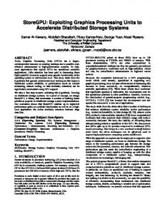
Table 4: Timing of the solution of the sparse linear systems introduced in Table reftable:sparseMatrices. To better understand the impact of the GPU on the overall multifrontal factorization, we take a closer look at the ibeam problem. The x-axis of Figure 8 represents different levels in the elimination tree of the ibeam matrix. The root is to the right at level 19 and the leaves to the left. The red curve is the sum of the number of frontal matrices at each level. It increases exponentially until it peaks near 7000 at level 7. A few leaves of the tree appear even deeper. The blue curve plots the sum of the floating point operations needed to factor the frontal matrices at each level of the tree. The integral of this curve is approximately 101 billion, the total number of operations needed to factor the ibeam problem. It is clear from the figure that the vast majority of the operations are in the top five levels. In fact 60 frontal matrices in the top six levels of the tree exceed the threshold for use of the GPU. Nevertheless, they comprise 65% of the operations. Figure 9 depicts the sum of the time spent at each level of the ibeam elimination tree. The red curve again represents the sum off all of the supernodes at each level. The yellow curve is the time spent assembling frontal matrices and stacking their Schur complements. These are the overheads associated with using the multifrontal method. The blue curve is the total time spent at each level of the tree when running on the host. The difference between the blue and yellow curves is the time spent factoring the frontal matrices. The brown curve is the time spent at each level of the elimination tree when using the GPU to factor the frontal matrices. The difference between the brown curve and the yellow one is the time spent on the GPU. It is clear from looking at Figure 9 that the GPU is very effective at reducing the time spent factoring the large frontal matrices near the root of the elimination tree. The difference between the brown and blue curves is the 52.5 seconds by which the 14
Figure 8: Number of supernodes and factor work at each level of the ibeam elimination tree.
GPU accelerated the overall factorization. Another way to look at he results is the throughput achieved, rather than the time reduced. Figure 10 also contains a red curve enumerating the frontal matrices at each level of the elimination tree. Instead of time spent, it plots the sustained performance achieved at each level. The blue curve is the performance achieved on the host. The purple curve is the factorization performance of the host, without the overheads of assembling and stacking. Notice that the performance of the host increases gradually as it climbs the tree and peaks at approximately 1 GFLOP/s. The brown curve in Figure 10 is the performance achieved at each level of the tree at which the GPU is used. The yellow curve is the factorization performance of the GPU. At level 14 in the tree, it is no faster than the host. But as it climbs the tree, it very quickly differentiates itself. The GPU factors the root at 14 GFLOP/s, and still sustains 13 GFLOP/s when one includes the time to assemble the frontal matrix.
6
Summary
This paper has demonstrated that a GPU can in fact be used to significantly accelerate the throughput of a multi-frontal sparse symmetric factorization code. We have demonstrated speed-ups as high as 1.97 for factorization, and 1.86 overall
15
Figure 9: Number of Supernodes and time spent factoring each level of the ibeam elimination tree.
Figure 10: Number of supernodes and throughput at each level of the ibeam elimination tree.
16
when accounting for preprocessing of the matrix and the triangular solves. This was done by designing and implementing a symmetric factorization algorithm for the GeForce 8800 in NVIDIA’s new CUDA language and then offloading a small number of large frontal matrices, containing over half the total factor operations, to the GPU. We believe that by demonstrating that the GPU can be successfully exploited in the multifrontal code, we have taken the next logical step beyond the pioneers who first implemented linear algebra kernels. Therefore, the authors consider the work described herein to be a major step on the road to exploiting GPUs in scientific and engineering applications such as MCAE. However, more work needs to be done before the use of GPUs will be common for the numerical aspects of such applications. The work reported here is in single precision, and most science and engineering sparse solvers operate in double precision. This could be addressed in several ways. Iterative refinement can also be used for well-conditioned problems [14] and [15]. Double precision can be emulated in software [16]. Ideally, future generations of GPUs will be extended to implement double precision in hardware. Similar devices, e.g., the Clearspeed [17], already do. The GPU frontal matrix factorization code implemented for this experiment should be revisited to make it more efficient in its use of memory on the GPU. It should be modified to implement pivoting so that indefinite problems can be factored entirely on the GPU. Further, it should be extended to work on frontal matrices that are bigger than the relatively small device memory on the GPU, much as the multifrontal code goes out-of-core when the size of a sparse matrix exceeds the memory of the host processor. And of course, the GPU ought to be integrated into the MCAE applications that use multifrontal solvers. Finally, if one GPU helps, why not more? Researchers have been implementing parallel multifrontal codes for over two decades [18]. In fact, the multifrontal code used in these experiments has both OpenMP and MPI constructs. Therefore exploiting multiple GPUs is not an unreasonable thing to consider. However, when one considers that one would have to simultaneously overcome both the overhead of accessing the GPU as well as the costs associated with communicating amongst multiple processors, it may be very challenging to efficiently factor one frontal matrix with multiple GPUs.
7
Acknowledgement
The authors wish to thank the following Norbert Juffa, Ian Buck, Ke-Thia Yao, Jacqueline Curiel for their helpful discussions, comments and edits. This material is based in part on research sponsored by the Air Force Research
17
Laboratory under agreement number FA8750-05-2-0204. The U.S. Government is authorized to reproduce and distribute reprints for Governmental purposes notwithstanding any copyright notation thereon. The views and conclusions contained herein are those of the authors and should not be interpreted as necessarily representing the official policies or endorsements, either expressed or implied, of the Air Force Research Laboratory or the U.S. Government.
References [1] M. T. Heath, E. Ng, and B. W. Peyton, “Parallel algorithms for sparse linear systems,” SIAM Rev., vol. 33, no. 3, pp. 420–460, 1991. [2] A. E. Charlesworth and J. L. Gustafson, “Introducing replicated vlsi to supercomputing: the fps-164/max scientific computer,” Computer, vol. 19, no. 3, pp. 10–23, 1986. [3] D. Pham, T. Aipperspach, D. Boerstler, M. Bolliger, R. Chaudhry, D. Cox, P. Harvey, P. Harvey, H. Hofstee, C. Johns, J. Kahle, A. Kameyama, J. Keaty, Y. Masubuchi, M. Pham, J. Pille, S. Posluszny, M. Riley, D. Stasiak, M. Suzuoki, O. Takahashi, J. Warnock, S. Weitzel, D. Wendel, and K. Yazawa, “Overview of the architecture, circuit design, and physical implementation of a first-generation cell processor,” IEEE Journal of SolidState Circuits, vol. 41, no. 1, pp. 179 – 196, 2006. [4] A. Lastra, M. Lin, and D. Manocha, Eds., ACM Workshop on GeneralPurpose Computing on Graphics Processors. Los Angeles, CA, USA: ACM SIGGRAPH, 2004. [5] I. S. Duff and J. K. Reid, “The multifrontal solution of indefinite sparse symmetric linear,” ACM Trans. Math. Softw., vol. 9, no. 3, pp. 302–325, 1983. [6] J. J. Dongarra, J. Du Croz, S. Hammarling, and I. S. Duff, “A set of level 3 basic linear algebra subprograms,” ACM Trans. Math. Softw., vol. 16, no. 1, pp. 1–17, 1990. [7] E. S. Larsen and D. McAllister, “Fast matrix multiplies using graphics hardware,” in Supercomputing ’01: Proceedings of the 2001 ACM/IEEE conference on Supercomputing (CDROM). New York, NY, USA: ACM, 2001, pp. 55–55.
18
[8] K. Fatahalian, J. Sugerman, and P. Hanrahan, “Understanding the efficiency of gpu algorithms for matrix-matrix multiplication,” in HWWS ’04: Proceedings of the ACM SIGGRAPH/EUROGRAPHICS conference on Graphics hardware. New York, NY, USA: ACM, 2004, pp. 133–137. [9] N. K. Govindaraju and D. Manocha, “Cache-efficient numerical algorithms using graphics hardware,” Parallel Comput., vol. 33, no. 10-11, pp. 663–684, 2007. [10] G. Karypis and V. Kumar, “A fast and high quality multilevel scheme for partitioning irregular graphs,” SIAM J. Sci. Comput., vol. 20, no. 1, pp. 359– 392, 1998. [11] C. Ashcraft and R. Grimes, “The influence of relaxed supernode partitions on the multifrontal method,” ACM Trans. Math. Softw., vol. 15, no. 4, pp. 291–309, 1989. [12] M. G. Arnold, T. A. Bailey, J. R. Cowles, and M. D. Winkel, “Applying aeatures of ieee 754 to sign/logarithm arithmetic,” IEEE Trans. Comput., vol. 41, no. 8, pp. 1040–1050, 1992. [13] I. Buck, “Gpu computing: Programming a massively parallel processor,” in International Symposium on Code Generation and Optimization, 2007, p. 17. [14] J. H. Wilkinson, Ed., The algebraic eigenvalue problem. USA: Oxford University Press, Inc., 1988.
New York, NY,
[15] A. Buttari, J. Dongarra, J. Kurzak, P. Luszczek, and S. Tomov, “Using mixed precision for sparse matrix computations to enhance the performance while achieving 64-bit accuracy,” ACM Trans. Math. Softw., vol. 34, no. 4, pp. 1–22, 2008. [16] Y. Hida, X. S. Li, and D. H. Bailey, “Algorithms for quad-double precision floating point arithmetic,” in ARITH ’01: Proceedings of the 15th IEEE Symposium on Computer Arithmetic. Washington, DC, USA: IEEE Computer Society, 2001, p. 155. [17] J. L. Gustafson, “The quest for linear equation solvers and the invention of electronic digital computing,” in JVA ’06: Proceedings of the IEEE John Vincent Atanasoff 2006 International Symposium on Modern Computing. Washington, DC, USA: IEEE Computer Society, 2006, pp. 10–16. [18] I. S. Duff, “Parallel implementation of multifrontal schemes,” Parallel Comput., vol. 3, no. 3, pp. 193–204, 1986.
19