Multilevel Projection Methods for Partial Differential ...

Downloaded 12/22/15 to 198.11.29.166. Redistribution subject to SIAM license or copyright; see http://www.siam.org/journals/ojsa.php

Stephen F. McCormick University of Colorado, Denver

Multilevel Projection Methods for Partial Differential Equations

SOCIETY FOR INDUSTRIAL AND APPLIED MATHEMATICS PHILADELPHIA, PENNSYLVANIA

1992


CBMS-NSF REGIONAL CONFERENCE SERIES IN APPLIED MATHEMATICS A series of lectures on topics of current research interest in applied mathematics under the direction of the Conference Board of the Mathematical Sciences, supported by the National Science Foundation and published by SIAM. The Numerical Solution of Elliptic Equations Bayesian Statistics, A Review R. S. VARGA, Functional Analysis and Approximation Theory in Numerical Analysis R. R. BAHADUR, Some Limit Theorems in Statistics PATRICK BILLINGSLEY, Weak Convergence of Measures: Applications in Probability J. L. LIONS, Some Aspects of the Optimal Control of Distributed Parameter Systems ROGER PENROSE, Techniques of Differential Topology in Relativity HERMAN CHERNOFF, Sequential Analysis and Optimal Design J. DURBIN, Distribution Theory for Tests Based on the Sample Distribution Function SOL I. RUBINOW, Mathematical Problems in the Biological Sciences P. D. LAX, Hyperbolic Systems of Conservation Laws and the Mathematical Theory of Shock Waves I. J. SCHOENBERG, Cardinal Spline Interpolation IVAN SINGER, The Theory of Best Approximation and Functional Analysis WERNER C. RHEINBOLDT, Methods of Solving Systems of Nonlinear Equations HANS F. WEINBERGER, Variational Methods for Eigenvalue Approximation R. TYRRELL ROCKAFELLAR, Conjugate Duality and Optimization SIR JAMES LIGHTHILL, Mathematical Biofluiddynamics GERARD SALTON, Theory of Indexing CATHLEEN S. MORAWETZ, Notes on Time Decay and Scattering for Some Hyperbolic Problems F. HOPPENSTEADT, Mathematical Theories of Populations: Demographics, Genetics and Epidemics RICHARD ASKEY, Orthogonal Polynomials and Special Functions L. E. PAYNE, Improperly Posed Problems in Partial Differential Equations S. ROSEN, Lectures on the Measurement and Evaluation of the Performance of Computing Systems HERBERI' B. KELLER, Numerical Solution of Two Point Boundary Value Problems J. P. LASALLE, The Stability of Dynamical Systems-Z. ARI'STEIN, Appendix A: Limiting Equations and Stability of Nonautonomous Ordinary Differential Equations D. GOTTLIEB and S. A. o RSZAG, Numerical Analysis of Spectral Methods: Theory and Applications PETER J. HUBER, Robust Statistical Procedures HERBERI' SOLOMON, Geometric Probability FRED S. ROBERI'S, Graph Theory and Its Applications to Problems of Society

GARRETT BIRKHOFF, D. V. LINDLEY,

(continued on inside back cover)


(continued from inside front cover) Feasible Computations and Provable Complexity Properties Lectures on the Logic of Computer Programming ELLIS L. JOHNSON, Integer Programming: Facets, Subadditivity, and Duality for Group and Semi-Group Problems SHMUEL WINOGRAD, Arithmetic Complexity of Computations J. F. C. KINGMAN, Mathematics of Genetic Diversity MOKI'ON E. GUKI'IN, Topics in Finite Elasticity THOMAS G. KuKI'z, Approximation of Population Processes JERROLD E. MARSDEN, Lectures on Geometric Methods in Mathematical Physics BRADLEY EFRON, The Jackknife, the Bootstrap, and Other Resampling Plans M. WOODROOFE, Nonlinear Renewal Theory in Sequential Analysis D. H. SATTINGER, Branching in the Presence of Symmetry R. TEMAM, Navier-Stokes Equations and Nonlinear Functional Analysis MIKLOS CSORGO, Quantile Processes with Statistical Applications J. D. BUCKMASTER and G. S. S. LuDFORD, Lectures on Mathematical Combustion R. E. TARJAN, Data Structures and Network Algorithms PAUL WALTMAN, Competition Models in Population Biology S. R. S. VARADHAN, Large Deviations and Applications KIYOSI ITO, Foundations of Stochastic Differential Equations in Infinite Dimensional Spaces ALAN C. NEWELL, Solitons in Mathematics and Physics PRANAB KUMAR SEN, Theory and Applications of Sequential Nonparametrics LAsZLO LovAsz, An Algorithmic Theory of Numbers, Graphs and Convexity E. W. CHENEY, Multivariate Approximation Theory: Selected Topics JOEL SPENCER, Ten Lectures on the Probabilistic Method PAUL C. FIFE, Dynamics of Internal Layers and Diffusive Interfaces CHARLES K. CHUI, Multivariate Splines HERBEKI' S. WILF, Combinatorial Algorithms: An Update HENRY C. TUCKWELL, Stochastic Processes in the Neurosciences FRANK H. CLARKE, Methods of Dynamic and Nonsmooth Optimization ROBEKI' B. GARDNER, The Method of Equivalence and Its Applications GRACE WAHBA, Spline Models for Observational Data RICHARD S. VARGA, Scientific Computation on Mathematical Problems and Conjectures STEPHEN F. MCCORMICK, Multilevel Projection Methods for Partial Differential Equations JURIS HARIMANIS, ZoHAR MANNA,


Copyright 1992 by the Society for Industrial and Applied Mathematics All rights reserved. No part of this book may be reproduced, stored, or transmitted in any manner without the written permission of the Publisher. For information, write the Society for Industrial and Applied Mathematics, 3600 University City Science Center, Philadelphia, Pennsylvania 19104-2688.

Printed by Capital City Press, Montpelier, Vermont.

Library of Congress Cataloging-in-Publication Data McCormick, S. F. (Stephen Fahrney), 1944Multilevel projection methods for partial differential equations / Stephen F. McCormick (CBMS-NSF regional conference series in applied p. cm. mathematics ; 62) Includes bibliographical references and index. ISBN 0-89871-292-0 1. Differential equations, Partial—Numerical solutions. 2. Multigrid methods (Numerical analysis) I. Title. II. Series. QA377.M32 1992 91-39536 515`.353—dc20


Contents

v PREFACE 1

CHAPTER 1. Fundamentals 1.1 Introduction 1.2 Notation and Conventions 1.3 Prototype Problems 1.4 Discretization by Projections 1.5 Realizability and Nadal Representations 1.6 Interlevel Transfer Matrices 1.7 Error Measures

31

CHAPTER 2. Multilevel Projection Methods 2.1 Abstract Framework: The Multilevel Projection Method (PML) 2.2 The Multigrid Method (MG) 2.3 The Fast Adaptive Composite Grid Method (FAC) 2.4 Prototype Problems 2.5 Relaxation 2.6 Coarse-level Realizability and Recursiveness 2.7 Parallelization: Asynchronous FAC (AFAC) 2.8 Other Practical Matters 2.9 Summary

49 CHAPTER 3. Unigrid 3.1 Basic Unigrid Scheme 3.2 Multigrid Simulation 3.3 FAC Simulation 3.4 Performance Assessment 3.5 Caveats


iv

CONTENTS

61

CHAPTER 4. Paradigms 4.1 Rayleigh-Ritz 1: Parameter Estimation 4.2 Rayleigh-Ritz 2: Transport Equations 4.3 Galerkin 1: General Eigenvalue Problems 4.4 Galerkin 2: Riccati Equations 4.5 Petrov-Galerkin 1: The Finite Volume Element Method (FVE) 4.6 Petrov-Galerkin 2: Image Reconstruction

97

CHAPTER 5 . Perspectives -

101 REFERENCES 103

APPENDIX A. Simple Unigrid Code

107

APPENDIX B. More Efficient Unigrid Code

111

APPENDIX C. Modification to Unigrid Code for Local Refinement

113 INDEX


Preface

This monograph supplements my recent book, published in SIAM's Frontiers series (Multilevel Adaptive Methods for Partial Differential Equations, STAM, Philadelphia, 1989) . The basic emphasis of that book is on problems in computational fluids, so it focuses on conservation principles and finite volume methods. This monograph concentrates instead on problems that are treated naturally by "projections," for which I have in mind finite element discretization methods. The eigenvalue problem for a self-adjoint diffusion operator serves as a prime example: it can be discretized by posing the problem as one of optimizing the Rayleigh quotient over the unknown projected onto a finite element space. This monograph shows that the projection discretization methods lead naturally to a full characterization of the basic multilevel relaxation and coarsening processes. That is, if we use the projection concept as a guide, the only basic algorithm choices we will have to make in implementing multigrid are certain subspaces that will be used in relaxation and coarsening. All other major components (e.g., interlevel transfers, coarse-level problems, and scaling) are determined by the projection principle. The Frontiers book and this monograph served as the basis for the lectures I gave at the CBMS-NSF Regional Conference on "Multigrid and Multilevel Adaptive Methods for Partial Differential Equations," which was held at George Washington University, Washington, DC, on June 24-28, 1991. The purpose of the conference was to introduce the participants to the multigrid discipline, primarily in terms of multilevel adaptive methods, and to stress general principles, future perspectives, and open research and development problems. In tune with these objectives, this monograph lays the groundwork for development of multilevel projection methods and illustrates concepts by way of several rather undeveloped examples. This monograph contains no serious treatment of theoretical results because it would be inconsistent with our objectives which is fortunate because almost no theory currently exists for multilevel projection methods. An outline of this monograph is as follows:

Chapter 1 includes motivation, notation and conventions, prototype problems, and the abstract discretization method. v


vi

PREFACE

Chapter 2, which is the core of this book, describes the abstract multilevel projection method, its formulation for both global and local grid applications, and various practical issues. Chapter 3 describes the unigrid algorithm, which is an especially efficient computational tool for designing multilevel projection algorithms. Chapter 4 develops several prototype examples of practical uses of these methods.

Chapter 5 identifies a few open research problems relevant to multilevel projection methodology. The development here assumes a basic understanding of multigrid methods and their major components, including discretization, relaxation, coarse-grid correction, and intergrid transfers. An appropriate foundation for this understanding is given in [Briggs 1987] . I am endebted to the National Science Foundation for support of the Regional Conference under grant DMS-9015152 to the Conference Board of the Mathematical Sciences and George Washington University. I am also thankful for the support of my research, on which this monograph is based, by the Ai Force Office of Scientific Research under grant AFOSR 86-0126 and by the National Science Foundation under grant DMS-8704169. I am especially endebted to the Conference Director, Professor Murli M. Gupta, who convinced me that his idea of having this conference was an excellent one, and whose leadership made it such a success. My gratitude also goes to several colleagues whose advice and guidance were essential to my completion of this monograph: Achi Brandt, Gary Lewis, Tom Manteuffel, Klaus Ressel, Ulrich Rüde, John Ruge, and Gordon Wade. I am also grateful to the typist, Mary Nickerson, whose skills and editorial suggestions greatly improved the final product. Finally, I could not have finished this work without the patience and support of my loving wife Lynda, and for that I thank her. Stephen F. McCormick University of Colorado, Denver


To Mom


CHAPTER

1

Fundamentals

1.1. Introduction. This monograph should be considered a supplement to the recent SIAM Frontiers book [McCormick 1989] on multilevel adaptive methods. That book contains a basic development of multilevel methods focused on adaptive solution of fluid flow equations. As such, it concentrates on finite volume discretization and multilevel solution methods that are compatible with physical conservation laws. Since many of the approaches of that book are relatively well developed and analyzed, it contains both numerical examples and underlying theory. Historical notes and references are also included. The emphasis of this monograph, on the other hand, is on what we call multilevel projection methods. The classical prototype is the standard fully variational multigrid method applied to Poisson's equation in two dimensions, using point Gauss-Seidel relaxation, bilinear interpolation, full weighting, and ninepoint stencils. (See [Stüben and Trottenberg 1982; §§1.3.4, 1.3.5, and 2.4.2], for example.) The key to understanding our basic idea here is that each stage of this prototype algorithm can be interpreted as a Rayleigh-Ritz method applied to minimizing the energy functional, where the optimization is taken as a correction over the continuons space projected onto certain subspaces of the fine-grid finite element space. In the stage where relaxation is performed at a given point, the relevant subspace is the one generated by the "hat" function corresponding to that point. In the coarsening stage, the relevant subspace is the coarse-grid finite element space. In general, the Rayleigh-Ritz approach, and the related Galerkin and PetrovGalerkin discretization methods, will act as guides to our development of corresponding relaxation and coarse-grid correction processes. These multilevel components will be developed in a way that is fully compatible with the projection discretization method that defines the fine-grid problem. One of the attributes of this approach is that the fundamental structure of all of the basic multilevel processes are in principle induced by the discretization. This can substantially simplify multilevel implementation, and it often provides the foundation for a very efficient algorithm. The central idea behind multilevel projection methods is certainly not new.


2

CHAPTER 1

Specific forms for linear equations have actually been known since the early stages of multigrid development (cf. [Southwell 1935] ), and they have recently been used for eigenvalue problems [Mandel and McCormick 1989] and constrained optimiza tion [Gelman and Mandel 1990] . Moreover, the basic idea is so natural and simple that it undoubtedly has had at least subconscious influence on many multigrid researchers. Yet, in almost all cases, specific forms of the projection concept were posed only in a Rayleigh-Ritz setting (however, see [McCormick 1982] , which used a Galerkin formulation) on global grids (however, see [McCormick 1984] and [McCormick 1985] , which consider the locally refined grid case) . In any event, this monograph represents the first attempt to formalize and systematize projection methods as a general approach, incorporating Rayleigh-Ritz, Galerkin, and Petrov-Galerkin formulations as well as global and locally refined grids. Actually, even the material developed here can be considered only as a first step in this direction. We do not as yet have a full set of general principles for guiding the choice of specific procedures, or a founding theory. Nevertheless, numerical results for a few examples suggest that these projection methods have significant potential. In any case, their consistency with discretization methods is a seductive premise for further exploration. As a supplement to the Frontiers book [McCormick 1989] , this monograph will be fairly brief. Included are certain parts of that book needed here for emphasis, and the central development will for the most part be self-contained. In fact, to some readers (especially those most familiar with finite elements), it would be best to start with this monograph. However, the Frontiers book should be consulted for background, history, related reference material, a few numerical illustrations (based on multilevel schemes that are generally not of projection type), and theory (that actually does apply to projection methods, if only in the linear self-adjoint case). Those who are unfamiliar with multigrid methods and their basic concepts should begin by reading more introductory material (cf. [Briggs 1987]) . One of the simplicities of the following development is that it is set primarily in the framework of subspaces of the relevant continuum function spaces. Thus, the discretization and solution methods are developed mostly in terms of finitedimensional subspaces of the function spaces on which the partial differential equation (PDE) is defined. This avoids some of the cumbersome notation (e.g., intergrid transfer operators) necessary when the nodal vector spaces are considered. In fact, the abstract methods apply even in cases where grids are not the basis for discretization (e.g., spectral methods). However, for practical relevance, we will occasionally use the nodal representation to interpret the concepts in terms of two prototype problems we shall introduce. Another simplification is to restrict our attention to spatial problems. Timedependent equations may be treated in a natural way by the projection methods developed, similar to the finite volume approach described in the Frontiers book. However, there is no doubt that much is to be gained by exploiting further the special temporal character of these problems, and it is perhaps better to postpone their treatment until this avenue has been more fully pursued. .


FUNDAMENTALS

3

Yet another simplification is to assume homogeneous Dirichlet boundary conditions for the PDE. (We will assume throughout this monograph that they are automatically imposed on all functions and nodal vectors. Along with this premise, we assume that all grids are "open" in the sense that they do not contain boundary points.) This is a standard simplification made in the finite element literature, and we find it particularly useful here since: it avoids additional terms in the weak forms; it avoids questions regarding approximation of boundary conditions on a given grid; and it allows us to treat the admissible PDE functions and finite element functions in terms of the spaces and subspaces in which they reside. For the reader who wishes to consider inhomogeneous but linear boundary conditions, it is enough to determine how they are to be imposed on the finest level: coaxse-grid corrections should satisfy homogeneous conditions, even when the PDE is nonlinear. Since the fine-grid treatment of inhomogeneous boundary conditions is a classical question of discretization, we need not deal with it here. These simplifications are likely to leave some readers with a false sense of understanding of certain practical implications of the principles and methods we develop. For example, it will seem natural and simple for variational problems to adopt the principle that the coarse-level correction should be defined so that it does its best to minimize the objective functional. However, it may be very much another matter to discern what interlevel transfer operators and coarse-level problems this abstract principle induces, let alone what happens at the software level. In fact, there are usually a variety of ways to realize such principles that are theoretically equivalent but have rather different practical consequences. Since the focus of this monograph is on basic principles and concepts, we will allude only to a very few of these issues. Therefore, the reader interested in practical aspects, especially those intent on using the ideas developed here, should begin by translating these principles into terms associated with the nodal representation of the discretization. Understanding details of the related multilevel adaptive techniques as they are developed in the Frontiers book [McCormick 1989] may be useful for this purpose. 1.2. Notation and conventions. The notation will conform as much as possible to that of the Frontiers book. However, the emphasis of that book is on finite volume methods for physical conservation laws, which means that a large percentage of the development involves finite-dimensional Euclidean spaces, and only a small percentage is devoted to continuum quantities. This is just the reverse of the present situation, which stresses finite element subspaces (i.e., continuum quantities) and only occasionally references nodal vector spaces. We therefore abandon the use of Greek symbols for the continuum and instead use underbar to distinguish Euclidean quantities. Following is a general description of the notation and conventions, together with certain specific symbols, acronyms, and assumptions, used in this monograph. Regions and grids use capital Greek letters; spaces, operators, and grid points


4

CHAPTER 1

use capital Roman; functions use lowercase Roman; functionals use capital Roman; constants use lowercase Greek or Roman; and quantities associated with a finite-dimensional Euclidean space (e.g., matrices and nodal vector spaces) use underbar. Following is a description of the specific notation commonly used in this text. Since much of the development of concepts rests heavily on visualization, we have made several tacit assumptions about this notation that generally simplify the discussion, but are not otherwise essential. These assumptions are indicated in square brackets below; they are meant to hold unless otherwise indicated. h Generic mesh size [mesh sizes are equal in each coordinate direction] ; used in superscripts and subscripts, but may be dropped when understood 2h Coarse-grid mesh size

h

ref to the com osite grid , p ( formed as the union of global and local uniform grids of different mesh sizes)

h h =

SZ, [ h (Open) regions in_Rd [regions are simp ly con-

nected, d = 2]; SZ = closure; á = SZ\SZ = boundary; CSZ = complement H, H1, H2, Sh, Th Continuum function spaces (including discrete finite element spaces) Supp(v), Supp(S) ST S2h,h T2h,h

Support of the function v, union of the support of all functions in S Maximal subspace of S of functions whose support is contained in Supp(T) Subspaces common to coarse and fine levels: S2h,h = S2h n Sh T2h,h = T2h n Th ,

R, Rh K, Kh k kh ,

Objective functionals for variational problems Operators for strongly formulated equations Forms for weakly formulated equations

S 2 h, SZh, SZh Grids [9 2 hand9hare uniform; SZh is the union of its uniform subgrids (Ph^ = 92h U [Zh) [Zh is aligned with [ 2 h; grids "cover" their associated regions in the sense that the region is enclosed by the boundary of the grid] ; grids exclude Dirichlet boundary points; patch = local rectangular uniform grid; level = uniform subgrid (i.e., union of patches of same mesh size) ;

Pk,

Grid points (nodes) PS Orthogonal projection operator onto S


FUNDAMENTALS

W

)

5

function in the finite element space Sh which has the value one at grid point F and zero at all other grid points

(.,.), (• ^ •

L2() or Euclidean inner product, norm Energy norm, used only for Poisson's equation:

I IIUIII = 11VUII ij • li lh

Discrete energy norm associated with a selfadjoint positive-definite linear operator Lh:

lii U hijl

Hó (SZ)

I2h' I 2h

= (u h, L h U h ) 1/2 First-order Sobolev space of functions that satisfy (in the usual Sobolev sense) homogeneous boundary conditions: Hó (SZ) = {u : liuji and II Vuil defined, u/OP = 0} Intergrid transfer matrices (interpolation, restriction)

(Vi, V2)V Multilevel V-cycle with vl and v2 relaxations before and after coarsening, respectively I Identity operator (on continuum function spaces) I Identity matrix L* Operator adjoint L t Matrix transpose a

V Divergence operator: V = ff in two di-

mensions

ay

0 Laplacian operator: 0 = V • V n, Rh Euclidean space of dimension n, Euclidean space corresponding to the grid of mesh size h -rh Full approximation scheme tau correction term (cf. [Brandt 1984] ) S°° Space spanned by elements of S

We will also use standard set notation, including 0 (the empty set), V gor every), E (contained in), c (is a subset of), (is not a subset of), n (intersect), and \ ( intersect the complement of). To avoid iteration subscripts, approximations such as u are dynamic quantities that can change assignment in an algorithm by a statement of the form u — G(u). This is understood to mean that the new assignment of u is the result of applying G to the old one. A superscript asterisk (*) on a vector is used to denote exact solutions and the symbol e is reserved to denote error. For example, uh — eh = uh* represents


6

CHAPTER1

the relationship between the approximation uh and exact solution uh* on Sh. The various unknowns, errors, and error measures used in this monograph are as follows: u* Continuum solution (on H) uh*

Discrete solution (on Sh)

uh Discrete approximation (in Sh)

e Actual error: e = uh — u* e* Discretization error: e* = uh — u* eh Algebraic error: eh = uh — uh *

r Residual error: r = K(u) ER,

ER, EK, EK

Error measures: ER (e) = R(uh) — R( u *), ER(eh) = R(uh) — R ( u h* ), EK ( e ) = IJK(Uh) II,

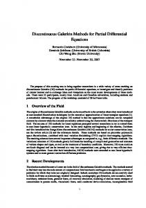
EK(eh) = IIKh(uh)II We should point out that the term multilevel has typically been used in the open literature as a generalization of the term multigrid. The term multigrid usually refers specifically to methods that are applied to the solution of PDEs discretized on a given (fine) grid and that use global relaxation schemes and global coarse grids for corrections. Our use of the term multilevel refers to a slight generalization of this type of method, which includes the case that the discretization uses a composite grid (e.g., consisting of uniform coarse and fine grids; see Figure 1.1) and relaxation on one or more levels is restricted to the local uniform grids. Acronyms used in this monograph are included below: AFAC Asynchronous FAC AMG Algebraic multigrid method BLAS

Basic linear algebra subroutines (cf. [Dongarra et al. 1979]) .

FAC

Fast adaptive composite grid method

FAS

Full approximation scheme

FMG Full multigrid method FVE Finite volume element method GML MG

Multilevel Galerkin or Petrov-Galerkin method Multigrid method

PDE

Partial differential equation

PML

Multilevel projection method

RML

Multilevel Rayleigh-Ritz method

UG

Unigrid

WU

Work unit

Algorithms used here include:


FUNDAMENTALS

t

FIG. 1.1. Simple composite grid.

AFACh C! Di! FACh Gh GMLh MGh PMLh RMLh

Asynchronous FAC Coarse-grid correction Directional iteration Fast adaptive composite grid method Relaxation (block Gauss-Seidel) Multilevel Galerkin or Petrov-Galerkin method Multigrid method Multilevel projection method Multilevel Rayleigh-Ritz method

Prototype problems. To provide a concrete understanding of the concepts developed here, we will illustrate them in terms of two simple prototypes, a linear equation and an eigenvalue problem, both involving the Laplacian. Let H1 and H2 be appropriate Hilbert spaces of function defined on the unit square, SZ = [0, 1] x [0, 1] . For simplicity, we assume that each function, u, in H1 1.3.

CHAPTER 1


8

in some sense satisfies the homogeneous Dirichlet condition u(z) = 0, z E aPLet L : Hl -- H2 be defined by Lu = —Du, u E Hl, and suppose that f E H2 is given. Then the prototypes we consider are given by (1.1)

Lu = f, u E Hl,

and (1.2)

(u, u)Lu = (u, Lu)u, u E Hi.

Here, (•, •) is the L2 inner product on H1. (We have chosen to write the eigenvalue problem using a form that is defined on all of Hl, including the origin. This simplifies treatment of both (1.1) and (1.2). However, it should be kept in mind that we are in fact seeking some nonzero u E H1 that satisfies (1.2) and for which the eigenvalue A = ù U^` is minimal.) To recast these equations in the forms suitable for projection methods, define KL : Hl —+ H2 and KE : Hl —* H2 as follows: (

(1.3)

KL(u)=Lu—f

and (1.4)

KE (u) = (u, u) Lu — (u, Lu) u.

Then, with K(u) denoting either KL (u) or KE (u), our two prototypes can be written collectively as the equation (1.5)

K(u)=0, uEHl.

We will make use of the weak form of (1.5), which is developed as follows. DefinetheformskL:H2 xHl -->RandkE:H2 xHl —^SJRby

(1.6)

kL(v, u) = (VV, Vu) - (v, f )

and (1.7)

kE(v, u) = (u, u) (vv, vu) — (vu, vu) (v, u).

With k(v, u) denoting either kL(v, u) or kE(v, u), then corresponding to (1.5) is the weak form (1.8)

k(v,u)=0, uEHI, VvEH2.

Natural choices for the function spaces associated with kL and JEE are Hl = H2 = H - Hó (9), the first-order Sobolev space of functions on SZ satisfying


FUNDAMENTALS

9

the homogeneous Dirichlet boundary conditions. In this case, we have the weak form

(1.9)

k(v, u) = 0, u E H, b'v E H.

A major advantage of the weak forms (1.8) and (1.9) over the strong form (1.5) is that their admissible function spaces (i.e., Hl and H, respectively) may generally be larger. For example, the form kL requires only first-order differentiability of u in the L2 sense, while KL requires second-order differentiability presumably everywhere. ' This difference is essential to the discretization process: kL admits continuous piecewise linear functions, while KL does not in the classical sense. We will have occasion in this monograph to discuss (1.5), (1.8), and (1.9) collectively. In order to avoid the inconvenience of including both the strong and weak forms, we will instead refer to (1.5) with the understanding that its meaning may be in the weak sense. Specifically, whenever we refer to (1.5), it should be understood that the equality may not be meant in the classical sense: whenever the stronger form is not strictly defined, K(u) = 0 will instead be taken to mean (v, K(u)) = 0 for all v E H2 or, in the transformed sense, k (v, u) = 0 for all v E H2. This is to be understood for (1.5) and any equation derived from it. For example, if P and Q are projection operators, then by PKQu = 0 we may mean k(Pv, Qu) = 0 for all v E H2. The definition of the operator PKQ itself may be meant in this context, that is, PKQu is the element of PH2 satisfying (v, PKQu) = k(Pv, Qu) d v E H2. To recast these equations in their variational form, consider the functionals 9:Hl -->Randm:Hl --*Rgivenby

e(u) = IJVU112 and where is the L2 norm on H1. Assume that f E H2 and define the functionals RL : Hl -+ R (energy) and RE : Hl \ {0} -+ R (Rayleigh quotient) as follows: (1.10)

RL(u) _ £(u) - 2 (u, f)

and (1.11)

RE(u) _

±^ m(u)

Note that, for appropriate u, KL(u) and KE(v,) are proportional to the respective gradients of RL(u) and RE(U). Then, with R(u) denoting either RL(u) or


10

CHAPTER 1

RE (u) and H denoting Hl, our prototype variational problems can be written collectively as the variation (1.12)

R(u) = min R(v), u E H. vEH

For the eigenvalue case in (1.12), technically we should replace H by H \ {0}. We assume this to be understood. Also for this case, the variational form amounts to specifying that we are targeting only the smallest eigenvalue of L = —z. For definiteness, we will henceforth add this constraint implicitly to (1.5), (1.8), and (1.9). For example, with K = KE, we take (1.5) to mean: "Find a nonzero solution of KE (u) = 0 with smallest A = There are several important properties of the prototypes that make the general problems suitable for the numerical discretization and solution methods we are about to develop. For example, all formulations for the prototypes have certain ellipticity properties that generally guarantee unique solvability (up to a scale factor for the eigenproblem) . In order to maintain more generality, and because we are not concerned here with theoretical issues, no assumptions of this kind will be introduced for the general formulations, (1.5), (1.9), or (1.12). However, it should be understood that some of these properties (e.g., that R has a minimum) are necessary for our discussion to make any sense. An interesting way to generalize (1.12) would be to add constraints. In fact, the eigenproblem already has the implicit restriction u 0, although this simple constraint has little impact on the numerical process we will develop. In general, however, the introduction of constraints leads to greater complexity in the number and type of numerical solution methods. We therefore restrict this monograph to the unconstrained case. (For recent work in the direction

of projection methods for constrained optimization, see [celman and Mandel 1990].) 1.4. Discretization by projections. One of the basic principles of multilevel methodology is to design the coarsegrid correction process in a way that is compatible with the discretization method. This is not a firm principle: there are instances where it is advantageous to use a coarsening technique that is in some ways superior to the discretization scheme, particularly when the latter is inaccurate; consider the double discretization methods in [Brandt 1984, pages 103-106]; also, the algebraic multigrid method (AMG) is based on a variational-type coarsening, but applied to matrices that do not necessarily arise from this type of discretization. However, this coarsening principle does provide a general multilevel design criterion that can lead to very effective algorithms. In any case, it is natural to relate two discrete levels guided by the discretization itself. To be more specific, but speaking loosely, suppose we are given a general discretization procedure, which relates the PDE (in weak or strong form) to a given discrete problem on level h (either finite element or nodal vector spaces) .


11

FUNDAMENTALS

By this is meant that we are given a mapping (possibly a projection) from the PDE space, H, to the level h space, Sh, and, just as important, that we also are given a mapping from Sh to H. Write these mappings as Qh : H ~ Sh and Qh : Sh ~ H, and suppose that we have analogous mappings for the subspace S2h of S", Then the relationship between levels 2h and h is defined by constructing interlevel transfers for which the diagram in Figure 1.2 commutes. That is, we define Q~h : Sh ~ S2h and Q~h : S2h ~ Sh implicitly by Q2h = Q~h . Qh and Q2h = Qh . Q~h' Of course, we must be sure that these definitions are realistic, that is, that these interlevel transfer operators are easily implemented. For the conforming projection methods considered here, this is certainly true as we shall see; in fact, this is one of the major motives for our focus on projection techniques. In addition to determining interlevel transfers, the problem must be specified on each level. The attempt to be compatible with the procedures used to define the fine-level problem leads us to choose the level h problem simply as the one that is induced by the discretization. This is the approach taken in this monograph. As we shall see, the form that the coarse-level problem takes is often a generalization of the fine-grid form precisely because the coarse-level unknown is an approximation to the fine-level error, not its solution; that is, the coarse-level correction is of the form u h + u 2h , and the presence of u h t- 0 creates a term in the coarse-level problem that is not generally present on the fine level (unless the problem is a linear equation or quadratic variation).

H

S2h

.....;;..:.::....-

__

Q~h FIG.

1.2. Discretization/coarsening diagram.

One of the main purposes of the foregoing discussion is to emphasize that, for projection discretization methods, taking this compatibility approach actually dictates the major coarsening components, which consist of the intergrid transfer operators and coarse-grid problems. We will see that this approach also guides the choice of relaxation. To be sure, other multilevel components must be determined, including the type and schedule of cycling, the possible use and placement of local grids, and the method of evaluating integrals and other quantities that must be approximated. The proper choice of these other components is no doubt critical to performance. But the major effort in applying multilevel methods is almost always devoted to the correct choice of coarsening and relax-


12

CHAPTER 1

ation. Thus, being guided by the projection scheme substantially narrows the focus of decision making. This does not mean that we have trivialized the task of multilevel design; in fact, proper choice of the underlying subspaces for relaxation and coarsening may be far from obvious. Nor have we fully committed ourselves to the projection approach; approximations to it, and even wholly new types of coarsening, may be better in some circumstances. However, it is very useful to begin the task of multilevel design with a formalism to guide the major choices. The task could then focus on determining the relaxation and coarsening subspaces that work together quickly to eliminate all error components. We will illustrate the results of several such design tasks in Chapter 4. This somewhat lengthy motivation brings us up to the description of projection discretization methods. Starting first with the equation, (1.5), let Sh C Hl and Th C H2 be finite-dimensional subspaces (possibly of different dimension) and let PS h : Hl -+ Sh and PT h :.H2 ---* Th be orthogonal projections onto Sh and Th, respectively. Then the projection discretization of (1.5) is given by the finite-dimensional problem PTh K(Ps h u) = 0, u E H1.

(1.13)

Let Kh : Sh --+ Th be given by Kh(uh) = PT hK(Ps huh) = PT hK(uh), uh E Sh. For example, assuming the case Th = Sh, then Kh (uh) = Lhuh — f h, where Lh = PS h LPS h and f h = Ps h f . Remember that the definition of Lh may be meant in the weak sense. Similarly, K(uh) = (uh, Mhuh)Lhuh — (uh, Lhuh)Mhuh, where Lh = PShLPSh and Mh = PSh. Then (1.13) can be rewritten as Kh (uh) = 0, uh E Sh .

(1.14)

Note that the weak interpretation of (1.13) or (1.14) is k(PThv,Pshu) =0, uEH1, VvEH2.

(1.15)

Defining kh(v h , uh) - k(PThv h , PShuh) = k(vh, u h ), uh E S h , vh E Th, then this becomes (1.16)

O(vh,

u") = 0,

uh E Sh,

`d vh E Th.

We refer to any of these discrete , formulations, (1.13)—(1.16), as the PetrovGalerkin form. In the special case Sh = Th, they will be referred to as the Galerkin form. The projection discretization of the variation, (1.12), is simply (1.17)

R(Psh

u) = min R(Ps h v), u

E

H.

Ej

Let R h (uh) - R(Psh uh) = R(uh ), uh E 8 k'. For example, Rh (uh) = (uh, Lhuh) —

f h ), where Lh and f h are defined as above. Similarly, RE(uh) = C u

2(uh,

Then (1.17) can be rewritten as (1.18)

Rh(uh)

= min v ES

Rh(vh),

uh E Sh .

hhh u

>


FUNDAMENTALS

13

We refer to either (1.17) or (1.18) as the Rayleigh-Ritz discretization of (1.12). The notation we have used thus far is suitable for discretization on a given global uniform grid. Since a major emphasis of this monograph is on local refinement methods, we now turn to the development of the projection discretizations suitable for composite grids. To this end, let Sh and S 2 h be nontrivial finitedimensional subspaces of Hl and let T" and T 2 h be nontrivial finite-dimensional subspaces of H2. We suggest by this notation that Sh and T" correspond to global uniform grids of mesh size h, and that S 2 h and T2 " correspond to their uniform subgrids of mesh size 2h, because this situation is typical of many multigrid implementations. However, none of these properties are really necessary for our discussion: none of the levels need be uniform, the mesh ratios can be different from 2, the coarse levels need not be subgrids of the fine level, and the fine grids may be local. Nevertheless, for simplicity of development, we will henceforth assume that the subspaces are conforming, which for the case that the fine grid is global is characterized by the assumption that (1.19)

S2h C S h and T2 h C Th.

Consider the case where the fine-grid regions Supp(Sh) and Supp(Th) may be proper subregions of 9. Here, Supp(S) = U VES Supp(v), where Supp(v) is the maximal subregion of SZ on which v is nonzero (i.e., the support of v). Let Ssh and TTh denote the subspaces of S 2 h and T 2 h of functions whose support are contained in Supp(Sh) and Supp(Th), respectively. Then by conforming in this general case we mean that (1.20) Supp(S) = Supp(S h ), Supp(T 2 h) = Supp(T h ), Ssh C Sh, and TTh C Th. The first two of these rather technical relations ensure that the grid interfaces for the local regions Supp(Sh) and Supp(Th) are actually coarse-grid Tines. Note that (1.19) is just a special case of (1.20). Now define the composite grid spaces by (1.21)

Sh = S 2h + S h and T! = T 2 h + Th.

Here we use zenderbar on h for denoting the composite grid vector of subgrid mesh sizes,

h =2h h Note that S! = Sh and T! = T" in the global grid case because we are assuming the conforming property, (1.19). Note also that, in general, the sums in (1.21) are not direct because S 2 h fl Sh 0 and T 2 " n T" 0. (In fact, in the global grid case, S 2 h fl Sh = S 2 h and T 2 " f1 T" = T 2 ".) This observation is important to understanding the limits to parallelizability of the fast adaptive composite


14

CHAPTER 1

grid method (FAC) and the motive for the modifications to it that lead to asynchronous FAC (AFAC). We will briefly discuss these points in Chapter 2, §2.7. (See [McCormick 1989, pages 129-133] for a more thorough discussion.) The composite grid problem that we wish to solve is either the equation, (1.14), or the variation, (1.18), but posed now on the composite grid space, Sh and T . In particular, letting H (uh) = PT h H(Ps h uh ), ut E 8!!, and Rh (i!!) - R(Ps h uh ), uh E Sh, then two forms of the composite grid problem are the equation K!!(u!!)=O, u!!8!!,

(1.22) and the variation

(1.23)

Rh(uh) = min Rh(vh), 2!! E Sk v—E S—

Of course, (1.22) may be taken in the weak sense

(1.24)

kh(vh, uh) = 0, uh E Sh, `d vh E Th,

where k (v , uh) - k(PT hv , Ps hu:!), u! E Sh, u!! E T& 1.5. Realizability and nodal representations. Both the Petrov-Galerkin and Rayleigh-Ritz discretization methods are deceptively simple, primarily because we are dealing here with projections and subspaces. We have not yet faced the issue of how these discretizations are to be represented in a computational environment, which can be rather involved. The usual approach is to specify the subspaces Sh and Th by finite elements, choose a locally supported basis for each, then rewrite the discrete problem in terms of the coefficients of the unknown uh expanded in the basis for Sh. For example, for our prototype problems in the form of (1.5) or (1.12) on global grids, we may choose Sh = T" as the subspace of functions in Hl that are piecewise bilinear with respect to the cells of a uniform grid, SZh, on 9. For the basis, we would choose the usual hat functions, which are defined as follows. Let the global grid Q" have interlor nodes Ppq , 1 < p, q < n. Then the hat function associated with Ppq is the element w Q) E Sh that satisfies

P Pnq

wh (P) 1

-

0

PEfZ'\{Ppq }.

The computational problem associated with (1.14) is to find the coefficients, U q, in the expression (1.25)

uh

= Ë uqw(Q) R4=1

15


FUNDAMENTALS

such that n

(1.26)

k1 (w

)

E uP9 w(pq) =0

Vi, j E {1, 2, •

• • , n}.

p,q= 1

(Here we must consider the weak form, (1.16) , of (1.14) because Kh (w^ p9) ) is not defined in the classical sense. Remember that Th = Sh for both prototypes.) Let Rh denote the Euclidean space of dimension n 2 corresponding to the nodal vectors for grid S h . Then, for the linear equation prototype, (1.1), this computational problem can be written as (1.27)

Lh26h = fh, 26h E

Here, L h is the matrix whose (ij) — (pq) entry (i.e., entry in the row associated with and column associated with Ppq ) is given by

3

(1.28)

(Lh )

p=i, q=j

ij—p q = (VWh), VW^rq)) — — 1 max{Ip — ij, iq — I } = 1

0

otherwise,

uh is the vector of nodal values u, and f h is the vector with entries 1

(1.29)

f -

f (x, y)w (x, y) dxdy. 0 0

We used the bilinearity property of the form k for (1.1) to realize the equation (1.27), meaning that this property of k allows us to reduce (1.14) to an equation that is computationally expressible in the sense that all of the operations defining it are elementary. We call (1.14) realizable in this case, which is an important concept because it determines whether we can really begin to compute discrete approximations. Actually, we have not quite reduced problem (1.21) to elementary operations because integrals are involved in (1.29). The exact evaluation of f h is generally not possible, so in a strict sense (1.14) is not realizable. However, this is a classical situation to treat in practice: we can, for example, simply assume f has some property (e.g., f E Sh) that allows exact evaluation of the integral in (1.29), then use standard Sobolev space arguments to determine the error introduced by this assumption. (See [Ciarlet 1978, §4.1], for example.) To simplify discussion, and because discretization error does not directly concern us here anyway, we will make such an assumption throughout the remainder of this monograph. More precisely, we will henceforth assume that the discretization of any given function by formulas like (1.29) is done exactly. In fact, we also make similar implicit assumptions on other subprincipal terms in the PDE (e.g., coefficients) so that they do not by themselves prevent realizability of the discretization.


16

(

CHAPTER 1

To see that (1.14) is realizable for the eigenvalue problem, (1.2), we again use the basis expansion, (1.25), and consider the case k = kE in (1.26). A simple calculation using the bilinearity of the inner products defining kE yields

(1.30)

(I^h^ M h 26h)L h 2l h = (26 h , L h 26h^M h 26 h ^ 26h E h,

where L h and uh are defined as above, M h is the matrix whose (V) — (pq) entry is Biven by

ss h2 (1.31)

Mh) ,j

—ne =

36 h2 1h2 ssh 0

h (W h

(=j)' w (ne)% —

p=il 4 = j ip-2I+ ^4 — .7 I =1

^=^9—I=1 .7 otherwise,

and (-, •) denotes the usual Euclidean inner product on Rh . Computational forms for the discrete variation, (1.18), for both the linear and eigenvalue prototypes are easily obtained. This is done by way of the expresEn sion (1.25), which is used to define R h (uh) = Rh ,Q _ 1 u h wh , uh E Rh. For the linear prototype, (1.1), we have (

(1.32)

Rh(uh) = (26h, L h uh)

—

2(41h, ƒ h)^ uh

For the eigenvalue prototype, (1.2), we have (1.33)

Rh(Mh) _ (uh' Lh uh) h 7b E î ^. (uh,Mhu)

These are just the standard variational forms for - the matrix problems (1.27) and (1.30), respectively. In fact, (1.27) and (1.30) can be derived by setting to zero the gradients of the functionals defined in (1.32) and (1.33), respectively. These forms show that the variational discretizations of both our prototypes are realizable. Realizability does not hold in general, but there appear to be many important practical cases where it does, as illustrated in Chapter 4. In other practical applications, computable approximations to the coarsening strategy may be suitable. In any event, this concept will become more relevant in the next chapter, where we consider multilevel coarsening strategies based on projections. The issue then is realizability of the coarse-level problem, which is posed to approximate the fine-level error. This is different from realizability of the discretization, which is posed to approximate the continuum solution. However, it should become apparent that the two are very closely related, and that theory developed to ensure (approximate) coarse - level realizability will no doubt rest on an understanding of discretization realizability. To illustrate the procedure for constructing composite grid representations, consider the linear equation prototype, (1.1). The discretization of the weak


FUNDAMENTALS

J

17

form, (1.16), produces a matrix L h that has essentially the same entries as L h given in (1.28) associated with the uniform regions of the composite grid SZh = S 2 h U S h, i.e., at points of SZh \ rh, where rh = SZ 2 h l og h is the composite grid interface. The only special entries of Lh are those associated with the points of

rh. To see how these interface stencils can be generated, consider Figure 1.3, which depicts a typical point, Pij, in rh together with its composite grid neighbors. (Here we index points according to the fine-grid mesh size; for example, in Figure 1.3, PZ+ 1 + 1 corresponds to + (h, h).) Most of the coefcients of Lh corresponding to its ijth row can be determined by using symmetry of Lh and knowledge of the coefficients -in rows corresponding to the uniform region of SZh . For example, the coefficient corresponding to column i - 2 j is - 3 . As a more complicated example, consider row i + 1 j of j . It would seem to connect point Pi+ l to points PZ j±1 each with - . But Pij±i are slave points (i.e., their values are not free but are rather determined by neighboring values), so use of bilinear interpolation means that the node values there are defined to be the average of the node values at the interface neighbors (e.g., uh (PZ + 1) = (I^-h (Pij) + uh (PZ +2)) /2) . Thus, there are no columns labeled i j ± 1 in Lk. Instead, in row i + 1 j of Lh, the slave point PZ + 1 creates the additional coefficient - 6 in both columns ij and i j + 2. Thus, the coefficient in row i + 1 j associated with is - 3 - - 6 = - 3 • Similarly, we can argue that the coefficient associated with in row i + 1 j + 1 is - 3 - s , where the second term comes from the coefficient of the slave point PZ j + 1, which is just - 21 . Continuing to row i + 1 j + 2, we see that the coefficient associated with PZ^ is - (via slave point PZ + 1) . Hence, by symmetry of Lh, the coefficients in row ij associated with points PZ+1 ^, PZ+1±1, P2+1±2, PZ-1 ^, and PZ-1±2 are _ 1 _ 1 _ 1 and -1 respectively. This leaves determination of the coef2 1 3 1 35 3 3 fi t ficients associated with Pij±2, which can be made directly; a simple calculation of kh (wh , w 2 ) shows that Pij±2 = 0. Finally, the diagonal term must be (

)

such that the row sum is zero (because Sh contains functions that are constant

in a region surrounding and because L applied to such functions must be zero inside this region) . This implies that the entries for Lh in row ij associated with point Ppq are given by

3

p=i,q=j

-13 p=i-2,

Lh =

ij-rq

q=j, j±2

p=i+1, q=j 32 -1 2 p=i+1, q= j+1 - 61 p=i+1,q=j±2 0

otherwise.


18

CHAPTER1

2h '

h

i-2 j+2

i j+2

i+1 j+2

i+1 j+1

i-2 j

ij

i+l j

i+1j-1

i-2 j-2

i j-2

'i+-1 j-2

FIG. 1.3. Composite grid interface points (o denotes slave points).

1.6. Interlevel transfer matrices. In a few instances we will illustrate basic principles by way of nodal vector representations for the prototype problems. For this purpose, we will need to use notation for the relationships between the various levels, [ 2 h, flh, and nh • Consider first the global-grid case, S 2 h C SZh, and let R 2 h and Rh denote the respective Euclidean spaces of coarse-grid and fine-grid nodal vectors. Then, because we are using bilinear interpolation for the prototypes, the relationship between grid 2h and grid h is given by the matrix I2h : R2h sRh, which is defined as follows: '2h : u 2 h H uh, where uh is the nodal vector corresponding to uh E Sh, which is defined for P E SZh by u 2 h(P)

p E Stzn

uh(P) _ (u2 h(P — Po) + u 2 h(P + Po))/2

P ± Po E S2 2 h,

Po = P^ or (Uh(P —Pam ) + uh(P + Pa))/2

P.

P f P f Py E SZ 2 h.

Here, u 2 h E S 2 h is the function with corresponding nodal vector u 2 h, PP = (h, 0), and P. = (0, h). (By P±Po E SZ 2 h, we mean either P+Po E SZ 2 h or P—Po E S^ 2 h, or both; by P ± P, ± P. E SZ 2 h, we mean at least one of the possible four points is in SZ 2 h. This rather complicated notation is due largely to the need to account for boundary points.) The relationship from SZh to f1 2 h is given by the adjoint mapping,

(1.34)

2

h = (L2h)

'

19


FUNDAMENTALS

which is proportional to the so-called full-weighting operator (cf. [Stüben and Trottenberg 1982, pages 14-16, 27]) . It is easily verified that the definition of L h in (1.27) satisfies LZh = I2hLhl2h•

(1.35)

Equation (1.35) is referred to as the Galerkin condition; (1.34) and (1.35) together are called the variational conditions. (See [McCormick 1987, pages 132134].)

For the local refinement case, where 9 2 h flh, we need to define transfer matrices between levels SZ 2 h and SZh and between levels [V and Som. (Transfers between S 2 h and f will not be needed because of the way we pose the basic methods: corrections from either of these grids are collected in the grid h approximation, so these grids need not communicate directly between themselves.) Let Rh denote the Euclidean space of composite grid nodal vectors. The definition of I2h : R2 h Rh is analogous to the definition of I2h: I2h : , u 2h i, where uh is the nodal vector corresponding to uh E S!, which is defined for P E SZh by

u 2h(P) h(P) _ (u 2 h(P — Po) + u 2 h(P + Po))/2 (uh(P — Py ) + u(P +Pam ))/2

P E St 2 h

P f Pa E St 2 h,

Po=P 1,orPy P f P f Py E St 2 h.

Here we should emphasize that our construction of the finite element spaces implies that the interface between the coarse-grid (2h) and fine-grid (h) regions in S contains only coarse-grid points. Specifically, this interface, I'L = S 2 h n af lh, is defined as the set of coarse-grid points on the internal boundary, which is the boundary of the region covered by the local grid, SZh, excluding the real boundary

09. Let P be any point on the internal boundary. The boundary values for Sh are assumed to be zero, so uh E Sh implies that uh (P) = 0. Since each uh E Sh can be written as the sum uh = u 2 h + uh for some u 2 h E S 2 h and uh E Sh, then uh (P) = u 2 h (P) . In other words, the internal boundary is a coarse-grid line. This means that the midpoint between two neighboring coarse-grid points in Fh is treated in practice as a slave point: the value of uh there is imposed to be the average of uh at these coarse-grid neighbors. This constraint is automatically

incorporated into the definition of I2h given above. —+ Rh is given simply as follows: The definition of the matrix J::

I h : u h —> uh, where uh is the nodal vector corresponding to uh E Sh , which is defined for P E Q h by P^ P E SZh (uh(P) _ u11(P) otherwise. 1.0


20

CHAPTER 1

This represents an imbedding of Rh into Rk 2h and I : QhRh are defined as The restriction operators I h :h adjoints of interpolation:

h

I2h

Ihh t —2

and Ih = (h) —h —h t .

At the end of the last section, we illustrated how the composite grid matrix

Lh associated with the linear prototype, (1.1), may be constructed. It is not difficult to argue from basic principles, or from examining in detail the' matrix entries, that all of the grid operators satisfy the Galerkin principle. For example,

L h = IhLhlh and L2h

= I hh Lhl2h'

Noting the definitions for restriction as adjoints of the interpolation operators, we see that the variational conditions are satisfied between all grid levels, not just between h and 2h as certified in (1.34) and (1.35). 1.7. Error measures. An important but often underemphasized issue in numerical computation is the choice of error measures, which are used to assess and, in some cases, control algorithm performance. In many circumstances, this assessment can be

very sensitive to the specific choices made (although this tends to be less so for multigrid than it is for other methods, as we will shortly argue) . In any case, it is important that error measures be chosen that properly reflect the "real" goal of computation. Determining this goal is often subjective and heuristic, and almost always problem dependent, so there is little that can be said in any general or absolute sense. However, the importante of error measures in practice compels us to make a few observations. Although we include several relevant aspects in this informal discussion, our main objective is to make a few specific points about the nature of error measures for multilevel projection methods. While error in numerical simulation comes from many sources, our main concerns here are the errors arising from the discretization and from the algebraic solver. More precisely, in subspace terms, let u* E Hl be a solution of either form, (1.5) or (1.12), of the problem defined on H = Hl; let uh* E Sh C H be a solution of the discrete problem, (1.14) or (1.18); and let uh E Sh be an approximation computed at some stage of the iteration process applied to the discrete problem. Then the error that' concerns us here is the actual error e=

uh

—u*,


FUNDAMENTALS

21

which is the sum of the discretization error e* =

uh *

— u*

and the algebraic error eh = uh — uh * . We first discuss the problem of assessing directly the actual error, e. For problems posed in variational form, (1.12), a natural measure of e is derived by considering the deviation of the functional form, R(u'), from its minimum, R(u*) : ER(e) = R(uh) — R(u*) . Note that ER(e) = R( u * + e) which shows that ER(e) does in some sense estimate the error, e. (For simplicity here and elsewhere, we restrict our discussion to absolute error measures, which means that we must be careful to keep the problem scale in mind in order to correctly interpret the values that are obtained. It is often better to use a relative error measure, which divides the absolute measure by a quantity like R(u*) . This usually makes the measure independent of scale, but the appropriate relative error measure is dependent on the problem; e.g., when R(u*) = 0, we must use another factor that correctly expresses the goal of computation.) R(u*) generally cannot be computed exactly in practice, so performance tests using this measure must in most cases either estimate R(u*) numerically, or be restricted to artificial cases where R(u*) is known. Suitable estimates of R(u*) can be obtained by requiring accuracy from the numerical scheme that is much greater than the accuracy in R(u"). This generally means significantly decreasing the mesh size and dramatically increasing the number of algebraic iterations. Using this approach to assess performance amounts to comparing the approximations computed in practical tests (e.g., using realistic mesh sizes and a few iterations of the algebraic solver) to an approximation computed using many more algebraic iterations on a much finer grid. These tests often involve assessing error on a sequence of practical mesh sizes with the goal of confirming a certain order of convergence (e.g., ER(e) < ch for some c < 00 independent of h) . This approach is usually simple to implement, but it more or less begs the question by assuming beforehand that the scheme actually converges (in both the discretization and algebraic senses) . This difficulty can be circumvented by estimating R(u*) using other discretization and algebraic solver schemes that are known to provide accurate, if not fast, results. A strategy that is often safer and more useful is based on constructing a testbed of problems where the minimum is knówn. The ability to do this depends on the specific form of R(u), however. For the first prototype problem, (1.1), this can be done by choosing a suitably smooth function u* that is zero on the boundary of the unit square, then forming f - Lu*. The resulting functional R - RL, defined in (1.10) for this given f, then has u* as its minimizer.


22

CHAPTER 1

Moreover, the minimum value is just R(u*) = _(u*, f), which can often be determined analytically, or arbitrarily well by quadrature, for a broad clans of choices of u. Note that the definition of e, the bilinearity of the inner product, and the fact that Lu* = f together imply, for the functional defined in (1.10), that t(e) = t(u' u*) = R(uh) + (u*,f) = R(u h ) — R(u * ) = ER(e)• The significance of this observation is that using the performance measure ER(e) is equivalent to computing 111 e 11 I2, where H —* Q is the energy norm defined by IIIwI!! = th/ 2 (w), w E H. Note that these comments hold for problems of the form (1.1) based virtually on any linear self-adjoint operator L : H —* H, provided the energy norm is defined accordingly. The second prototype problem, (1.2), is simpler because its solution is known. In fact, u* (x, y) - sin(irx) sin(iry) is an eigenvector of L = —0 belonging to the smallest eigenvalue, A = 7r 2 , which is the minimum value of R = RE defined by (1.11). Unfortunately, the smallest eigenvalue of operators other than the Laplacian are seldom known, so one must generally rely on somewhat less secure performance measures for these cases. Even so, confidence in the effectiveness of an algorithm can be built by observing an anticipated order of convergente of an error measure based on some strategy for estimating R(u*), especially if

these observations are backed by theory. The ultimate goal in the algorithm design process is to develop an efficient scheme that produces an actual error of acceptable size. In this process, it is important to realize that the actual error consists of discretization and algebraic errors, which is expressed by the relation e=e*+eh.

If design begins by assessing the actual error of a practical scheme directly, then any possible deficiencies in performance cannot be easily traced to their sources. It is therefore important to be able to measure the individual error contributions from the discretization and the algebraic approximations. This would allow algorithm design to focus individually on the discretization and algebraic solver strategies. A natural measure of the algebraic error for the variational problem, (1.12), is given by ER(eh) = Rh(u) — Rh(uh* ).


FUNDAMENTALS

23

Note, as above, that

ER( e h ) = Rh(uh' + eh) — Rh( u h+ )• Again we may restrict performance tests to cases where R(uh*) is known. This is easy to do for the linear prototype, (1.1), because we can simply select any uh * E Sh and compute f h = Lhuh* by a matrix-vector product. Here, Lh = PS h LPS h (in the weak sense) . This determines Rh and its minimum, Rh (uh*) = _( u * , ƒh). Analogous to the actual error case, we note that this measure of the algebraic error is related to its energy norm as follows:

ER(e h ) _

IIlehIlI2.

In fact, (1.36)

ER(eh) _ I

where the discrete energy norm

I II ' lilh : S h —> ^t is defined by

w h lllh = ( W h , Lh W h) 1/2 7 wh E S h . These comments so far carry over virtually to any linear self-adjoint problem of the form (1.1). Again, the eigenvalue prototype problem, (1.2), is simpler because the smallest eigenvalue for the generalized discrete eigenproblem, (1.30), is known. In fact, a discrete eigenvector uh* E Sh can be constructed simply by interpolating the differential eigenvector given by u* (x, y) = sin(7rx) sin(7ry); that is, uh* is the unique element of Sh that agrees with u* at the nodes of SZh. Simple trigonometric identities then show that the smallest eigenvalue is

^ h = Rh(uh*) =

36(2 — cos(irh) — cos 2 (irh)) h 2 (4 +4 cos (7rh) + cos 2 (7rh)) '

which is an order h 2 approximation to A = 1r 2 , the smallest eigenvalue of (1.2). However, as in the actual error case, the smallest eigenvalues of other operators are seldom known. Thus, for problems of the form (1.12), we may in general be forced to use numerical estimates of R(uh*) . Analogous to the approach for actual error estimation, Rh (uh*) can be approximated by requiring more accuracy from the numerical scheme than is needed in practice, which translates in this case simply to more iterations of the algebraic solver. Again, this can be tricky because it presumes that the algebraic method converges, although other algebraic schemes that are known to converge may be used to confirm these estimates. The discretization error, e* = uh* — u*, associated with the variational form, (1.12), may be measured by the quantity ER(e*) R(uh*)

-

R(u*).


24

CHAPTER 1

To do this, we must now estimate both R(uh*) and R(u*), which can be done numerically by computing very accurate solutions on level h and on a much finer mesh, respectively. Once more it is important to be sure that these estimates are relatively accurate and not contaminated by weakness of the numerical scheme. Error measures other than the energy functional may of course be used. For example, if II - II denotes some norm on Hl (e.g., L2, energy, or Sobolev), then 1 leli may be used to measure the actual error, e* (1 the discretization error, and I l eh i j the algebraic error. Again, this is likely to involve estimates of the exact solutions, u* and uh* , or restriction to cases where they are known, so care must be taken with these measures. To improve confidence in these approximations, and to enhance error estimation generally, still other error measures may be considered. For variational problems of the form (1.12), the optimal solution is often a local extremum, that is, a solution of the gradient equation (1.37)

VR(u)=O, u E Hl.

This duality between minima of the variation and zeros of the gradient can be exploited to the benefit of the numerical solution of (1.12) by introducing error measures baséd on (1.37). Let • ( be some norm on H2. Then one possibility is to use the residual norm:

IJVR(u)11 measures actual error; V R(uh*) V Rh (uh) I

measures discretization error; and (

measures algebraic error.

These measures are appropriate when (1.37) can be taken in the strong sense. However, for the prototype problems and in many other instances, only the weak form of (1.37) holds. In such situations, we may still use the residual norm by way of the nodal vector representation: letting rh = V R h (uh) denote the residual for (1.37) and • 1( the Euclidean norm on W,, then measures the algebraic error in the approximation, uh, of the solution of (1.12). This measure has the practical significance that it is generally computable (assuming V R h (uh) is), so it can be used in production codes to assess and control performance. Unless the residual norm is used with care, however, it can give misleading results. To illustrate this potential difficulty, consider the linear prototype problem posed in its variational form, (1.10). Note that the residual error norm for the nodal gradient equation is rhll

= I

- J h )II,

where L h is the matrix whose entries are given by (1.28). Using the relation L h uh — f h = L h eh, then the algebraic residual error norm is given by (1.38)

iirhij = 2(eh,(Lh)2eh)1/2•

25


FUNDAMENTALS

On the other hand, the algebraic energy error norm is given by

I

(1.39)

= (eh,Lheh)h/2.

Now the real objective of the numerical process for solving (1.10) is presumably to achieve an acceptably small energy error. (This assumption is founded on the relation between the energy measure and energy error norm, (1.36), and the definition of the energy measure in terms of the variation.) This leads to the ideal convergence criterion

lijehilih 0 is some suitably small error tolerance. (e may correspond to any available estimate of the discretization error, lije*lij, or otherwise to a fixed reference, like machine epsilon or precision.) The energy error norm cannot be computed in most practical circumstances, so we are generally left with estimating it by the residual error norm. The point we want to make is that I ( rh I I yields a poor estimate of lij t^h ij I h . To see this, note that 1/2

I [

_2 ^h IIIh

^vh ^Lh vh ^ (vh,vh)

)

where vh = (Lh)h/2 e h which yields the sharp estimate

i rh 11 27^

Illeh Illh

0 is some prescribed tolerance. Remember that the actual error is the sum of the discretization and algebraic errors:

e=e*+eh. Then it seems reasonable to achieve our computational goal by ensuring both (3.6)

IIe* II < E

2

and (3.7)

liehij < 5

•

2

To require one to be significantly smaller than the other would be computationally wasteful. (Actually, a carefully tuned objective would take into account the problem dimension, the order of discretization accuracy, and the tost and convergence factors for the grid h and grid h/2 V-cycles; cf. [Brandt 1984, §7.2] . Such an analysis might suggest in some cases that the algebraic error tolerance be somewhat smaller than the actual error tolerance. However, it is seldom that these tolerances should differ by more than an order of magnitude, and, even in such cases, the principle underlying the following argument is basically the same.)


58

CHAPTER 3

Now (3.6) dictates the size of the mesh size, h. For example, if a bound on the discretization error is known to behave like ch 2 then (3.6) is achieved by choosing ,

1/2 h=

(3.8)

2c

(If c is unknown, it can be estimated by assessing typical discretization errors as described in Chapter 1, §1.7. Note that h might be chosen more conveniently as, say, the negative power of 2 closest to satisfying (3.8).) Assuming for discussion that h is chosen in this way, then (3.7) can be rewritten as

liehii< ch 2

(3.9)

.

This expresses the convergence criterion that can be difficult for algebraic solvers to achieve: given an initial guess (e.g., uh = 0) with error presumably of order 1, then even a solver with optimal algebraic convergence factors (bounded less than one independent of h) must perform on the order of log(1 /h) iterations to be sure that (3.9) is satisfied. FMG methods circumvent this trouble to achieve full optimality by using coarser levels first to determine a starting approximation for the V-cycles that is already fairly accurate: if u 2 h satisfies the 2h version of (3.9), then its actual error can be no worse than 8ch 2 (the sum of its discretization and algebraic error bounds), so it must approximate uh * by an error no larger than 9ch 2 thus, (3.9) can be achieved by just one V-cycle with a convergence factor bounded by 1/9. Thinking this through recursively leads to the FMG scheme that cycles from the coarsest to the finest grid, using a V-cycle on each level applied to the approximation computed on the coarser level. In a unigrid framework, using (0,1) V-cycles, this FMG scheme is written, analogous to (3.4), as follows: ;

For µ = 2, 3, • • • , p: For v=1,2,••• 5 11: For

1,2,•••,mh': uh

E--

Dh 2Gh; d h(e)v). (

Actually, (0,1) V-cycles are usually not sufficiently effective to reduce the error by 1/9. (1,1) V-cycles or (2,1) V-cycles are common in practice, but the best choice must be determined by numerical or theoretical analyses, or both. To summarize, thorough tests of the performance of a multigrid code should carefully estimate worst-case algebraic convergence factors of the basic cycling scheme and actual errors left in the results produced by the overall scheme. The tests should include a spectrum of mesh sizes and problem data (e.g., source terms and boundary conditions), and the estimates should be measured against the computational costs of achieving the desired accuracy.


UNIGRID

59

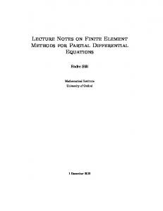
3.5. Caveats. Unigrid can provide a very useful tool for design of multigrid algorithms. It is especially effective for experimentation with several algorithm variants, inciuding different cycling strategies, local refinement, and various forms of relaxation. However, it has several limitations that should always be kept in mind. The major disadvantage of the unigrid method is its efficiency. A little experience with unigrid should convince anyone that it will seldom if ever be useful as a technique in production software. It is important to understand this slowness beforehand so that it never comes as an imposing disappointment. For example, the very long processing times stemming from unigrid inefficiency create a practical limitation on problem size that may be too restrictive to give full confidence in the multigrid performance that it is simulating. Another limitation of unigrid is its restriction to projection-based relaxation and coarsening processes. It is awkward if not practically impossible to try fundamentally different strategies in the unigrid context. The commitment to point relaxation methods would seem just as strong because unigrid corrections are based on single vectors, not subspaces. Actually, though, this is not quite the case. In fact, block relaxation can often be approximated by using either many unigrid relaxations within the block, or special unigrid directions that are designed to simulate multigrid within the blocks. For example, line relaxation on a given level can be accomplished by an inner unigrid scheme that involves one-dimensional "coarsening" of the directions associated with each line. (Note, for example, that the coarsest direction for relaxation on a level 2h y line is a skinny hat function that has support of width 4h in the x direction but extends up to both boundaries in the y direction. See Figure 3.2.)

FIG. 3.2. Support for coarsest-level hat function for y-line relaxation on level 2h.


60

CHAPTER 3

A third major difficulty with unigrid is that it circumvents the question of coarse-level realizability. Of course, this feature is just what makes unigrid so useful because it also avoids the need to construct this realization. However, for most studies, it will be essential to certify that the final algorithm design can be implemented in a code • that exhibits the usual multigrid complexity. This can often be proved analytically, but perhaps the most convincing argument is to produce the code itself. So, in later stages of development, it is often best to abandon unigrid in favor of a true multigrid implementation.


CHAPTER

4

Paradigms

We have carried along two important prototype problems in an attempt to illustrate the basic principles developed in the first three chapters. These principles and the techniques they induce have been very well developed and analyzed in the open literature for the linear problem, (1.1). To a lesser extent, this is also true for the eigenvalue problem, (1.2). However, these prototypes alone do not justify the effort which we have just undertaken to develop these principles into a general methodology. We therefore devote this chapter to exploring several other specific applications of the general approach. The paradigms described in the following sections are in widely varying states of development. While none is even close to being fully explored, some have progressed enough to show encouraging potential. Others, however, are currently just ideas. In any case, each of these examples will be presented in a fairly succinct way, with no numerical results, no theory, and little in the way of concrete motivation. We will attempt to present these paradigms in a clean and mostly formal way, choosing the simplest model problems and the most natural PML schemes, and being - vague about the relevant function spaces and other constructs. There are several risks taken here, not the least of which is that we are overlooking subtleties that threaten the soundness of the whole approach. In fact,

while this monograph was being written, we discovered an essential difficulty with our initial formulation of the parameter estimation problem. But, instead of describing our new approach to this problem, we chose to stay with the old paradigm because it provides an interesting example of how multigrid can expose trouble with existing mathematical models. After all, we are developing paradigms, with the sole central aim of illustrating the potential for the general methodology to apply to a wide variety of scientific problems; actual development of viable techniques, careful mathematical constructions, and overall proof of concept will have to walt for mach more study. This chapter develops six paradigms, two each using Rayleigh-Ritz, Galerkin, and Petrov-Galerkin projection schemes, presented in that order.

61


62

CHAPTER 4

4.1. Rayleigh-Ritz 1: Parameter estimation. PDEs are often found at the core of numerical simulation. In fact, the state of many physical processes can be described as the solution of a static or timedependent boundary value problem. Unfortunately, while the form of the PDE may be known, frequently the coefficients are not. Thus, one of the major tasks of mathematical modeling is to experiment with the real physical process under a variety of imposed conditions, observe specific behavior of the state of the system, then use these observations to deduce the unknown coefficients. A prime example of this inverse problem comes from electrical impedance tomography. The electrical voltage in a given conducting body is determined by imposed voltage or current fluxes on its surface. The voltage is known to obey an elliptic equation, where the coefficient represents the conductivity of the body. The tentral task in electrical impedance tomography is to estimate this coefficient by using observations from experiments that measure both the voltage and the current fluxes at the boundary, under varying conditions of state. Typically, a variety of flux conditions are imposed on the body's surface, and resulting voltages are observed there. The premise in inverse problems is that enough observations on the state of the system will make it possible to recover some of the details of the equations that govern it. In the case of electrical impedance tomography, these details are the interior values of conductivity, which yield an image of the object under study. We will use a special formulation of the inverse problem of this type that is applicable to two-dimensional steady-state elliptic equations. (See [McCormick and Wade 1991] .) This form, which was introduced in [Kohn and Vogelius 1987] , uses the variation m m -1 (4.1) R(a; u(.); v(.)) = > IIVV(k) 112 dz, a IIVU(k) 11 2 + a

(

where SZ Ci 2 is the unit square, • 1 1 is the L2 norm on R 2 , a is the conductivity parameter, and u(.) and v(.) are the state variables. a, u(.), and v(.) are assumed to lie in appropriate Hilbert spaces of functions defined on 9. (We use u(.) to denote u(k), k = 1, 2, • • • , m, collectively, and similarly for v(.) and other quantities that follow.) Let u^k) and vak) denote functions defined on the boundary, F, of SZ, 1 < k < m. Then the problem that we consider here is to minimize R in (4.1) subject to the restrictions

a>0 and (4.2)

U(k) = uk)

and V(k) =

on t,

10 and

U where uo and ()

)

and

V

on r,

)

vo are the respective interpolants of u^ ° and v o on the bound()

(

)

()

ary, JY , of 9h, 1 < k < m. (By u 0h being the interpolant of u° on I'h we mean that u° h is the unique function that is continuous piecewise linear with respect to the cells of rh and agrees with u° at its nodes.) To determine the discrete representation of Rh in terms of the parameter cell values and state nodal values, first note that the integral in (4.5) can be written as a sum of integrals over the cells of SZh, on each of which a is constant. Thus, a simple calculation based on writing the state variables as bilinear functions of their nodal values yields the expression m n

h

R h( a h ;u);v) )

h

/ h

k=1 i,j=0

(4.6)

+(a112112)-1 a ±i ,2±i , 2 (v)).

Here we have used the quantity a +1/2 +l/2 (uh), which is defined in terms of the differences 6hi+1/2 - uh (Uh) = u z-}-1 j+l uhz j+1 z+1 j j+1 Z3 bh (Uh) = ?.Gh• i+1/2 S2 +1/2

(uh) = u

+1

—u,

^ +1/2jt1/21^ h ^ -

and 6+ 1+l/2 (u h ) = u + 1 j+, l — uZ+ 1 j by

6 3 (( ^1/2j( uh )) 2 + + (51121(uh))2 + (6 j^-Fl/2ûh^^2 ^

ih

+ `îA+l/ 2 ^ uh ^^l^ +1 j+l/2^ uh ^^ + 1i +1./+1^2

0 < i, j < n. (We use half indices for cell centers, n > 1 to represent the number of interior grid Tines in both coordinate directions of SZh, and a +1/2 j+l/2 to denote the value of ah on cell i + 1/2 j + 1/2, 0 < i, j < n.) Note that (4.6) shows that the discretization of R is realizable. The simplest form of relaxation on (4.6) is fairly straightforward. State relaxation is conventional because, for fixed a, Rh is just a sum of discrete quadratic forms for 2m homogeneous diffusion equations. Thus, relaxation of one of the state variables is just standard point Gauss-Seidel applied to the associated homogeneous system of state. Note that individual state variables can be processed independently of the others. Parameter relaxation is even simpler. In fact, for fixed state, since there is no interaction between the cells

65


PARADIGMS

directly via the parameter, then (4.6) can be minimized exactly in one step by the formula

m

k=1

a112112

(4.7)

1/2

= k=1

0 < i, j < n. A sensible relaxation strategy for (4.6) is to first perform point Gauss-Seidel on each of the state variables, holding the parameter fixed, then finish with a relaxation on the parameter via (4.7). This process constitutes one full relaxation sweep for minimizing (4.6). It is also possible to use other more complicated relaxation strategies that involve interaction within the state variables and between the states and the parameter. The coarsening process is based on the subspace, S0 h , of S' of functions which are continuous piecewise bilinear with respect to the cells of S 2 h C SZh, and which are zero on %1 Here we assume that n> 1 is odd so that S 2 h is a conforming uniform subgrid of dimension (n — 1) /2 x (n — 1) /2. We also define Sah as the subspace of Sa of piecewise constant functions with respect to the cells of S 2 h . Then the natural coarse-grid correction functional is given by R2h/a2h. u 2h. v 2h1 _ Rh( a h . a2h; uh +

/4.81

u2h. vh + v2h1

a 2 h E Sa h , u S0 h , and v2 h E S0 h , 1 < k < (n— 1)/2. For the state variables, this uses the usual additive correction scheme. However, the parameter is treated by a multiplicative correction, which is more natural and which, as we now show, enables the correction to be coarse-grid realizable. To argue heuristically that R2 h is expressible in terms of a reasonable number of elementary Euclidean operations on S 2 h (the details of a constructive argument would require cumbersome notation and too much detail), consider a typical component of Rh, which we write as Qh(bh; wh) =

f bh(w^)

2

dz.

i

Here, bh E SQ represents either ah or (ah) -1 and wh E Sh (with wh = 2c^° h on F) represents one of the state variables. Note that Rh can be written as a sum of terms of this type and of the type f. bh(w) 2 dz, which is treated analogously. Now the component of R2 h corresponding to this term is given by Q 2h (b 2h i w 2h ) = Qh(bh . b2h; 2llh + 111 2 h),

b2 h E Sáh and w 2 h E S0 . This gives Q2h(b2h; w 2h) = (n-1)/2 b +1

I

2 1 2 (bh(wfl2+-

/

fr, 2h

i,j=0i+1/2j+1/2

(2bhwh)w

h

+bh(W 2h ) 2 ) dz,


66 CHAPTER 4

where p +1/2 j+1/2 is cell i + 1/2 j + 1/2 of Q 2 h, 0 < i, j < (n — 1)/2. This relation for Q 2 h shows that we may restrict our attention to a typical coarse-grid cell, Q +1/2 j+1/2, which corresponds to four fine-grid cells, SZ2 2+µ 2j+v , µ, v = 2 , 2 . Close inspection shows that R2 h is just a generalized form of the fine-grid variation, Rh, and that it is indeed expressible in terms of a reasonable number of Euclidean operations on SZ 2 h. In fact, the first term in Q 2 h, given by the expression (n-1)/2

bi+1/2 j+1/2f 2h z, b wx d h( h)2 2h rn,

i, j=0 i+1/2 j+1/2

is a linear term in b2 h, which Rh does not have. Note that the integral term in this expression is fust the cell SZZ+1/2 j+1/2 component of the fine-grid "residual" Rh ( ah; u^ ) ; we ) . The second term in Q 2 h, given by )

(n-1)/2

2h 2bi+1/2j+1/2 i,j=0

2h

h )WX2h , ( b h wdz

r,i+1/2 j+1/2

is bilinear with respect to (b2 h, w 2 '), which again has no counterpart in Rh since it corresponds to a nonzero source term for the elliptic equations of state. Finally, the third term in Q21', given by (n-1)/2 +1/2 j+1/2

bh (w)2 dz,

fr,2h i, j=0 1/2 j+1/2

is analogous to the individual cell terms in Rh, except for the integral weighting term bh. In any event, each of these terms can be easily evaluated by performing operations on grid 2h involving quantities that are computed and transferred from grid h at the beginning of the coarsening cycle. This gives the usual sense of grid 2h realizability. It should also be clear that this process is recursive: the coarsening of Q 2 h yields a grid 4h form that is analogous to Q21', so this heuristic argument extends to all coarser levels. To complete the formal development, we need to be sure that relaxation can be easily performed on all coarser levels. This is clear for parameter relaxation

because the parameter appears in R2 h in precisely the same form as it appears in Rh, so a relaxation formula analogous to (4.7) holds on coarser levels. For the state, it is enough to realize that each coordinate variable appears as a quadratic polynomial in R2 h. In fact, state relaxation is just Gauss-Seidel applied to the corresponding inhomogeneous elliptic equation with a source that arises from linear state terms in R2h. Unfortunately, while this formal development seems very natura!, our numerical experience with the RML scheme based on the functional, R, defined in (4.1) has been disappointing. The trouble here probably stems not from the

67


PARADIGMS

method, but from the functional itself: R seems to have such a degree of singularity in it that perhaps no natural approach will be able to determine its minimum effectively. This essential difficulty with R comes somewhat as a surprise because it has been appaiently overlooked by those who use it in practice, despite an otherwise careful analysis (cf. [Kohn and Vogelius 1985 and 1987]) . This paradigm is therefore all the more interesting as an example of how poor multigrid performance can expose trouble with the basic approach. To see this trouble clearly, we will consider a functional, defined only in terms of the state variables u(.) and v(.), that is equivalent to R, then assume we are so close to the minimum that the new functional is quadratic in state. First notice that if we are at a minimum, then the parameter in (4.1) must satisfy m 1/2

:i: liVv(k) 11

a=

2

k=1

(pointwise).

k=1 This shows that minimizing R in (4.1) is equivalent to minimizing the parametereliminated functional m

1/2 m 1/2

R(u;v) = f ^ IIVU(k) 112

^ IIVV(k) 12

dz.

k=1

Here we drop the subscript (•) for convenience, so u and v now stand for the respective u( k ) and V(k) collectively. For simplification, we abuse the notation further and rewrite R as

R(u;u)= f IJVull - J1Vvil dz, where u and v are now thought of as block vector functions with respective entries u( k ) and V(k), and the pointwise norms are given by m

1/2

m

1/2

IIVUII = ^ Ilouck>IIZ ana Ilovll = ^ Ilov(k^l 2 \k=1 ( k=1 (

Taking the Fréchet derivative of R(u; v) in the direction (p; q), then taking the Fréchet derivative of the result again in the direction (p; q), yields the Hessian form (4.․)

R"(u; v)(p; q) 2 = f IJ VU II. IIVVII[IIVp112 + IIV q 112- «Vu, ^p)


68

CHAPTER 4

where we use the notation (note that Vp and Vq are "normalized" by II Vuil and respectively) l

vu = vu/IlVuil, vv = vv/Ilovll,

= vp/Iloull, V = vq/Ilovll•

Now consider the one-observation case u = u( 1 ) = x and v = v( 1 ) = y:

R"(u; v)(p, 4) 2 = f [p +Pv + Qx + qv — (px — 4) 2 J dz =

[p2 + q + 2pxgyJ dz

=

[Py'+ q^] 2 dz,

where the last line follows from integration of the term pxqy by parts and the fact that p and q are zero on (9. Now the trouble is apparent: if we let P(x, y) = a'(x)Q(y) and 9(x, y) = —a(x)/3'(y),

where a = a(x) and f3 = f3(y) are any (suitably smooth) functions whose values and derivatives are zero at x, y = 0,1, then .FF(u;v)(p;q)2 = 0!

For example, we could take

a(x) = sin e k7rx and f3(y) = sin 2 £lry, so that p and q are as oscillatory as we like, yet (p; q) is a null-space component for f". If we now consider the case of the two observations u =

v=

1

y and let p = x

(

2-x y and

1

Pl and let q = ( q1 ) , then we obtain a similar )

p2

q2

result:

R"(u; v)(p; q) 2 =

si

—

pip + pi p + pL + p2^ + q? + q 2 + q2^ + q2^

_

_

pl x + p2 ^ ql^ q2x

dz

which, with the choice ql = — P2 and q2 = —pl and using integration by parts,

yields R"(p;q)(u;b)2 = 2

—p2)2dz;

69


PARADIGMS

this shows that null-space components for R" include

pi(x, y) = a'(x)13(y), 4i(x, y) =

-

a(x)^'(y),

p2(X, y)

=

42x, y) =

cx(x)f3'(y),

-

a'(x)Q(y),

where a = a(x) and 0 = fl (y) are as above. We speculate that this is typical of the situation for the general case of m > 1 observations of general type. Minimization of a functional with a Hessian that has an infinite-dimensional null space is not necessarily a problem. For example, it may be that the finite element space used to discretize the functional is in the orthogonal complement of the null space, in which case all of the usual discretization estimates and stability properties might be obtained in this complement. (The finite element space may also be allowed to contain null space components, provided the rest of the space is in its orthogonal complement.) Real trouble arises when the finite element space is arbitrarily close to the null space of the Hessian, without intersecting it. This means that the discrete Hessian has arbitrarily bad ellipticity (e.g., its condition number is much larger than O (h - 2 )) and that null-space components of the continuum Hessian are likely to contaminate critically the approximation of some or all of the well-posed components. This is the situation we face with the functional defined in (4.1) . We have therefore chosen to abandon this formulation of the parameter estimation problem in favor of the more conventional approach of output least squares, which we are just beginning to explore. As with most inverse problems, most forms of the parameter estimation problem are physically ill-posed. This is suggested by the fact that we are attempting to use boundary data to estimate quantities defined on the interior of the region. While it is true that knowledge of the exact Dirichlet and Neumann boundary values for a complete (and, therefore, infinite) set of observations may mathematically determine the parameter (cf. [Kohn and Vogelius 1985], which treats the function we defined in (4.1», physical and computational constraints limit the number of observations, the accuracy in the data, and the resolution and accuracy of the discrete system. As a consequence, it is essential to examine how these limitations and the problem's ill-posedness affect the numerical approximations—and even how we are to interpret the results that are obtained. We must therefore be more specific about what is meant by a solution to the problem, and this additional characterization must be effectively incorporated into the numerical scheme. Unfortunately, many conventional methods for handling this ill-posedness take a symptomatic approach that does not account for the specific source of the trouble. For example, the functional might be regularized by adding a term that tends to eliminate oscillatory parameter components, even though some oscillatory aspects of the parameter can be accurately estimated using the original functional. Based on an observation by Achi Brandt, we now suggest how the multilevel projection method can make parameter estimation problems well posed essentially by filtering out solution components that are not correctly determined,


70

CHAPTER 4

without harm to those that are. To do this, we must first characterize the wellposed components. Considering the physical model defined in (4.3), it is not difficult to see that any oscillatory behavior of the parameter has negligible effect on the state variables far from where this behavior occurs, relative to the scale of the oscillations. More specifically, if a is perturbed by a term that has zero mean but oscillates at a frequency of Oz in a region in SZ that contains the support of this term, then the change in any solution of —V aV u = 0 will be negligible at a distance of several Oz's away from this region. This suggests that the problem can be better posed by computing only those components of the parameter that are smooth in the interior of SZ and increasingly oscillatory near the boundary, F. The multilevel projection method can accomplish this by local refinement using fine-level grids that are increasingly local to I'. See Figure 4.1 for an illustration of the grids we have in mind. The PML scheme developed for solving most parameter estimation models can easily incorporate local refinement of this type in the regularization and solution process.

FIG. 4.1. Sample composite grid and its subgrids for parameter estimation.

4.2. Rayleigh-Ritz 2: Transport equations. Particle transport plays a fundamental role in many scientific fields, including nuclear reactor design, radiation therapy, semiconductor device modeling, and


PARADIGMS

71

satellite electronics shielding. The linear Bolzman transport equations govern the movement of neutrally charged particles. For steady-state, single group, isotropic scattering on the homogeneous semi-infinite slab [-1, 1] x (-00^ 00) 2 in R3 , if we assume that the particle flux, u, is independent of y and z, then these equations simplify to the following: (4.10)

Qs

1

µux (x, µ) + atu(x, p) = 2 u(x, v) dv + f (x, p),

where at and a s are constants (probability density cross-sections) satisfying 0 < a, < at , f is a given source, and the independent variables are the spatial distance, x, and the cosine of the angle from the x axis, M. We consider (4.10) on the region SZ = [-1,1] x [-1,1] subject to the following boundary conditions, which prescribe the flux of particles entering the slab:

(4.11)

u(-1,,a) = u°(µ), 0< p ah > 0) would be effectively treated by point Gauss-Seidel with the ordering along horizontal lines of grid cells, beginning for each line at its Dirichlet boundary (left end for positive µ, right end for negative p) . At the other extreme where at h is very large, if aa is small compared to at, then R' (u') is dominated by the influence of the mass matrix arising from the operator term atI in L. (I is the identity operator.) In this case, point Gauss-Seidel using any ordering and by itself, without multileveling, should be effective. When ut h is large and cri h is (nearly) equal to it, Rh (uh) is dominated by the influence of a matrix arising from the (nearly) singular operator cytI — u.,P in L, where P is defined by Pu(x, µ) = 2 f'1 u(x, v) dv. This suggests a ,u -line relaxation scheme, where, for each i in turn, the u are changed over all j E {±1, ±2, • • • , ± n} so that the resulting Rh(uh) is as small as possible. This relaxation scheme is particularly easy to perform since the resulting linear equation that defines this optimal change involves the 2n x 2n rank one matrix consisting of all ones. The interaction between different values of u occurs only through this matrix, so the linear equation defining /c-line relaxation is especially easy to solve. Taking all of these heuristics into consideration, a likely candidate for general at and a s is ei-line relaxation performed alternately from left to right and right to left. The coarsening of Rh is straightforward. In fact, L is linear, so R is quadratic in u. Thus, the coarse-grid correction process is entirely analogous to that for our linear prototype, (1.1) . Also, there is no special difficulty here with choice of the subspaces if S 2 h is a conforming subgrid of SZh (i.e., n is even) because the corresponding space of functions that are piecewise constant in g and continuous piecewise linear in x is a subspace of S'. Note that coarse-grid realizability and recursiveness are natural consequences of this observation. These ideas were developed in collaboration with Thomas A. Manteuffel. Theory has been developed in this simplified setting to show that R(u) exhibits a sense of ellipticity (i.e., il Lui l > y I u I for 'y > 0 and all suitable u) , which in combination with appropriate approximation * properties yields discretization error estimates. Also, based on earlier work with other multigrid techniques [Manteuffel, McCormick, Morel, and Yang 1990] , initial experiments are currently being conducted by Klaus Ressel using the above relaxation schemes and coarsening strategies. An important aspect of this study will be the use of composite grids to resolve boundary layers, internal layers, and other local phenomena present in many realistic transport models. 4.3. Galerkin 1: General eigenvalue problems. The second prototype problem, (1.2), is posed as one of finding the small-


PARADIGMS

75

est eigenvalue of a self-adjoint linear operator. Rom certain perspectives, this is fairly simple to treat, especially since a variational principle can be used. Fortunately, many practical problems are of this type, especially in dynamic structural analysis, in single-group neutron diffusion, and in modeling electron energy states. However, even a slight departure from this special case, like small convection terms in L, prohibits a variational formulation. Significant departure, such as when L is hyperbolic or nonlinear, may lose many of the well-behaved properties exhibited by our model: the eigenvalues can become complex, degenerate, or, in many ways, pathological; and the eigenvectors can become complex or generalized, or lose their subspace and completeness properties. It would be a formidable task to deal with these issues here. Instead, we will very briefly outline a formal approach to treating eigenvalue problems that does not depend on a variational principle. We will discuss only the formulation of the general problem and the abstract form of its discretization. We will not discuss other aspects of the multilevel projection method because they can be developed much in the same way that they were for (1.2). Also, we will not consider any of the fundamental questions that this formulation raises, such as which eigenvalue is to be approximated, whether continuation methods are necessary, and what grids and subspaces should be used for discretization. The only purpose of this discussion is to suggest a formal procedure for treating eigenvalue problems that are not of the same class as our prototype. In fact, we will focus on a general linear eigenvalue problem, although it should be clear that an analogous formulation may be applied to many nonlinear operators as well. Consider the generalized eigenvalue problem

Lu = AMu

(4.15) subject to the constraint

(u, Nu) = 1.

(4.16)

Here, L, M, and N are linear operators defined on an appropriate Hilbert space,

H, of functions equipped with the inner product (•, •) . Let H+ = H x R. Then the main point of this discussion is that (4.15)—(4.16) may be rewritten as the nonlinear equation

K(u+) = 0,

(4.17)

where u + = u E H+ and K is the operator on H+ defined by ()

u K()

Lu — ^Mu =

The discretization of K is based on a finite-dimensional subspace, Sh, of H. Letting S+ = Sh x R, then the Galerkin discretization of K is Kh (u+) PS+K(Ps+u+), u+ E S+. Noe that Kh 2L h = Kh

(uh)

Lh26h - J1hMh^h

^h (uh, Nhuh)-1 /+^ -

CHAPTER 4


76 u h ES h andA h E i ,where

Lh = PS h LPS h , Mh = PS h MPS h ,

and Nh = PS h NPS h .

Now the coarsening of Kh is given in terms of a subspace, S 2 h, of Sh and defined

onS 2 -S 2 hxRby

K 2 h (u+) = Ps+ K h (u+ +u),), u+ E S+ Writing u+ _

u 2h

^Zh ), then

(

K2h u2h —

( u''\

(

,\2h

Ah L2h u 2h — )2hM2h u 2h — )j hM2h u 2h — A 2 hPS2hM h u h + PS2h(L h u h — )hM h u h ) 2h 1 N2h u 2h) + (u 2h , PS2hN h u h ) + (N h PS2hU 2h 5 u h ) + (uh, Nhu h ) — 1 (u

Thus, the coarse-grid equation represents a yet more general eigenproblem, but in this generality this projection scheme is evidently coarse-grid realizable and recursive. In fact, these relations are just the Galerkin analogues of the RayleighRitz scheme applied to the prototype problem, (1.2).

4.4. Galerkin 2: Riccati equations. Consider the model linear quadratic regulator problem, which is defined in terms of the state, v = v(x, t), and control, w = w(t), by Minimize 00 pl

(VQV + rw 2 ) (x, t) dx dt

fo Jo subject to Vt = Av + bw on [0, 1] x [0, oo), v(0,t) = v(1,t) = 0, t >0, v(x, 0) = vO(X), 0

^ x ^ 1.

Here, Q is assumed to be an integral operator of the form 1

Qz(x) = i 4(x, ^)z(C) dC; n


PAR.ADIGMS

77

r is a constant, so without loss of generality we take r = 1; A is the onedimensional operator V • V = á ; and b = b(x) > 0 and vo (x) are given. The spatial functions are assumed to lie in some Hilbert space, H (e.g., H = L2[0,1]). The control solution, w, of this problem may be written formally in terms of the linear operator, U, applied to the state:

w = B*U v . Here we define the operator B: R - H by

Ba = ab, a E R, so that B* : H — R is the integral operator defined by

f

b()w() d.

The task is to find U, which may be a solution of the Riccati equation (assuming U and Q are self-adjoint):

AU + UA

—

UBB*U + Q = 0.

Now let L be the two-dimensional Laplacian, L = —V • V = —0. Suppose that U can be written as an integral operator, given by 1

Uz(x) _ i u(x, rj)z(^) dry, n

z E H. Suppose also that q and u are symmetric kernels in the sense that 4'(x, y) = 9(y, x)

and u(x,y) = u(y,x),

0 < x, y < 1. Suppose finally that q is nonnegative and u is positive in Q. Then substitution of the differential expression for A and the integral representations for U, B*, and Q into the Riccati equation leads to the following equation, whose

positive symmetric solution is presumably the kernel of U: (4.18)

K(u) - Lu + (B x u)(By u) — q = 0, u E H,

where Bu(x,y) =

f

b()u(,y)d


78

f

CHAPTER 4

and

çl

By u(x, y) =

0

b(rj)u(x, rj) drl.

Our discretization of K uses a uniform grid, flh, on SZ and the subspace,

Sh C H, of continuous piecewise bilinear functions with respect to its cells. The discrete operator is defined by Kh (uh) = Ps h K (Ps h uh ), uh E Sh. Note that

(4.19)

Kh(uh) = Lhuh + Psh (BxPshu h )(ByPshu h ) -- q h ,

where Lh = PShLPSh corresponds to the matrix defined in (1.28) and qh = Ps h q is the usual finite element source-term discretization (cf. (1.29». To examine the nonlinear term in (4.19), let wh 1 < i, j < n, denote the hat functions in Sh defined in Chapter 1, §1.5. We can write w(Z ^) (x, y) = w (i) (x)w(^) (y)

where w^Z) is the one-dimensional hat function associated with the uniform grid with mesh size h defined on [0,1], 1 < i, j < n. Define

1 (4.20)

bh =

in

b(^)w^Z) (^) d^,

1 < i < n. These coefficients will usually require approximation, unless the function b has special properties, for example, when b is a piecewise polynomial with respect to the cells of grid h on [0, 1] . Note, for piecewise constant b, that bh = (b((i — 1/2)h) + b((i + 1/2)h))h/2, 1 < i < n. Then, writing n

uh =

uh wh p4 (p4) p,q=1

and fixing i, j E {1, 2, • • • ,n}, we have

(w)' (B-„uh)(Blluh))

—

o

f

0

P9 =1

w(X)w

=1 P,4

(i) ( y )

u^bpw(a)(y) ^

,q=1

,9=1

4=1

n

n

^

uqwq)))

/ (B

(B (Z^)

bP w )' w (e)^^ P9

^ bq (w (=)' w (P)^ uáq ,q=1

Here, the one-dimensional inner products satisfy

1 2h/3

(Wk),W))

= h/6

0

k=2

Ik £1 = 1 -

otherwise.

u

q

b9w (n)

(x)


PARADIGMS

79

Hence, the nodal representation for PS h (Bx Ps h uh) (By Ps h uh) is given by (:Uxhgh) * (= By

uh ),

where, for 1 < i, j < n: * denotes vector products computed componentwise (i.e., (rh * w h) Z = vh . w h.. ); uh is the nodal representation of uh; Bh is the matrix defined by . ) C 421

( Uxhgh)= h (Z^) :

s r_ 1

h +u h 1 ) ; bh 1^ uh ` ^J 1 + 4u P^-^-1) PJ (

-

and B yh is defined analogously by

= ( 4.22 )

( Bhuh)(..) h q(

s

bu

Z—^

Q

+ 4u + u

1 q)

q =^

The discrete equation can thus be written as (4.23)

Lhuh + (gl&h) * (Bhuh) — qh = O.

Kh(uh)

Because of the quadratic nature of the nonlinearity, implementing point Gauss-Seidel on (4.23) is fairly straightforward. In analogy to (2.18), the ijth step involves finding an s E that soloes (Ighj)3 h (uh + s4^ )) = 0. Z K

(4.24)

)

It is easy to see that (Wh

j)j

Kh(uh+84f) )) =r

+d^s+c^s 2 ,

where r = (!4 ), Kh(uh)) = (LhUh + (BXMh) * (RYMh) qh)(Z^),

(4.25)

d = L -Z^ + 3 b^ (Bh uh )i + 3 bZ (Bhu h )^, ch -

-

4

9 bZb^.

Hence, one root of (4.24) is given (in numerically accurate form) by (4.2s)

s=—

2r d2-+ (dij )2 -4r^c

This root corresponds to the correct step size in the linear limiting case b - 0. The computational complexity of the discretization in (4.23), which is the coat of evaluating K h (uh) for a typical uh, is O(n2 ). This follows Erom observing

CHAPTER 4


80

that the nonlinear terms in Kh have the same O(nz) complexity as the linear terms: for example, the quantity in (4.21) coats O(n) to compute, but it needs to be evaluated only for each of the n rooms of u (i.e., for j = 1, 2, • • • , n). In this light, a straightforward implementation of point Gauss-Seidel is generally too expensive because the quantities in (4.25) must be computed at a cost of O(n) operations for each of the na grid points, yielding a total cost per sweep of O(n3 ). The culprit here is that the terms in (4.21) and (4.22) must be recomputed for each of the n 2 points. When the nonlinear terms in (4.23) do not dominate the discretization, a leas costly scheme is determined by the linear limiting case, which gives the step site 3=—

r L ij—ij i.!

It is, hoorever, generally more effective to use (4.26) but freeze the nonlinear terms computed in (4.25) over each full relaxation sweep. Another possibility is to use a global relaxation scheme skin to Richardson's or Jacobi's method. For example, uh could be corrected in the direction wh - K h (uh) using the step-size criterion (Wh, K h (9l.h + 340h)) = O.

A third possibility is simply to implement point Gauss-Seidel by computing the quantities in (4.25) initially for all points, then using inexpensive update formules to correct them locally after the iteration step at each point is performed. In any case, all of these alternatives are O(n 2 ) in complexity and should exhibit good smoothing, provided the nonlinear terms in the discretization are not too dominant. (Point relaxation is generally a poor smoother with respect to the nonlinear terms, so other relaxation processes must be considered when these terms dominate.) Assume that n> 1 is odd, so that the uniform subgrid , S 2 h C S h , conforms to 11. Let S 2 h be the subspace of Sh corresponding to SZ 2 h. Then the coarse-grid operator is defined in principle by Kuh (?^ Zh ) - PszhKh(Uh + u2h), 262 h E S 2 h, Let 1'h _ Kh(uh) and q2h = Ps2r.rh. Define Bih and Byh in analogy to the respective definitions of Bi and B in (4.21) and (4.22). (Note that if b is piecewise constant with respect to the cella of, SZh, then by (4.20) we have

b29 =(b((2i— )h)+3b((2i— )h)+3b((2i+ )h)+b((2i+ )h)).) Now define the functions ,D

Ps2i1 Bx uh and 3y2 h

Pgah By uh and the grid 2h linear

operator

k2h = L2h +Qs h B^ h + /3b h B^ h •

Then it is easy to verify that K^n (14 2 h) = k2h U 2h + (Bx2h U 2h)(BV h u2h) — q2h.


PARADIGMS

81

Thus, the coarse-grid operator has a form (and complexity!) analogous to the fine-grid operator, except that the linear part is modified by linear integral operators. In any event, this establishes both coarse-grid realizability and recursiveness. The prospects for developing an effective Riccati solver based on multilevel projection methods seem to be very good. If the usual multilevel convergence rates can be achieved, then a total computational complexity of order n 2 should generally be attainable. That is, we should be able to compute the matrix corresponding to the Riccati integral operator to an accuracy comparable to discretization error at a cost proportional to the number of nonzero coefficients in the fine-grid operator. This is the usual complexity property of multigrid methods. Actually, we may even be able to do much better with local refinement. To suggest this, it may be in many cases that the Riccati kernel u(x, y) is smooth as a function of x and y when l x — yI 0. For such x and y, u can therefore be well approximated on coarser levels, and it should be possible to use a composite grid that is increasingly finer near the diagonal line x — y = 0. Figure 4.3 depicts an example based on using triangular elements, which conform better than rectangles to the diagonal geometry. In cases where enough accuracy can be obtained by restricting the finer levels to just a few elements on either side of the diagonal, we may be able to develop a PML scheme for computing the Riccati kernel with a total computational complexity on the order of n log n. That is, by using a composite grid with O (n log n) points, we may be able to produce an approximation with actual accuracy comparable to that of the solution of the n x n global fine grid.

»

FIG. 4.3. Example two-level composite grid for the Riccati kernel.

The research work on this topic is in its -early stages, with only preliminary numerical results obtained thus far (cf. [Ito, McCormick, and Tiejun 1991]). Encouraged by early success for the simpler cases, the ultimate aim is to see


82

CHAPTER 4

how far these principles will carry into higher dimensions (e.g., foor- and sixdimensional equations of the form (4.18)) and more sophisticated PDEs (e.g., advection-diffusion and Navier-Stokes equations). 4.5. Petrov-Galerkin 1: The finite volume element method (FVE). In this section, we develop a multilevel projection method based on the finite volume element (FVE) discretization technique, which was used in the Frontiers book [McCormick 1989] to treat Huid flow equations. We use the interpretation of FVE as a Petrov-Galerkin scheme to provide the basis for GML. The development may seem a little awkward because the naturel approach to coarsening (i.e., the naturel choice of toeree-grid spaces) leads to technical difficulties (e.g., nonconforming elements)—and this we avoid by taking a coarsening approach that is perhaps more algebraic than physical. The method that results from this approach is different from, and lees natural than, the physically based multigrid scheme developed in the Frontiers book. Nevertheless, this paradigm is useful if for no other reason than to illustrate one possible general mechanism for dealing with nonconforming elements. Consider the two-dimensional Poisson equation K(u) _ –Du – f = 0, u E H,

(4.27)

where H is an appropriate Hilbert spare of functions defined on the unit square, S2 C 2 , that have zero values on BSZ. Actually, we take (4.27) in the following weak eense. For any suitable control volume, V c S2, define its characteristic function by vlr (z)

(1

zEV

t 0

otherwise.

Note formally that (vv, K(u)) =

f vv(z)(–Lu(z) – f (x)) dz t

=

f(z)dz, v JO V (–Du(s))ds–

where n is the ontward unit normai on 0V. Define n•• (–Vu(s» ds – v f (z) dz.

k(vv, u) =

J

Then by (4.2?) we really meen the weak form

(4.28)

k(v^, u) = 0, u E Hl, b'v E 112,


PARADIGMS

83

LIII FIG .

4.4. Grid, triangulation, and sample control volume.

where Hl is possibly a different Hilbert space of functions defined on [Z with zero values on OSZ, and H2 is the set of characteristic functions of suitable control volumes in 9. The discretization of (4.28) is based on: a uniform grid, SZh = {Zij : 1 i, j < n}; the space of continuous piecewise linear functions, Sh c Hl, associated with a triangulation of S2h; and the set of characteristic functions of the square

control volumes corresponding to SZh, which we write as Th = {VhZ : 1 1 and m > p > 1. Then the discrete ray depicted in Figure 4.7 corresponds to one of the equations in the discrete system

(4.35)

Lh7dh = J h , uh E Sh^


PAR.ADIGMS 89

where Lh = PThLPSh and f h = PT h f . Note that the row corresponding to this discrete ray has nonzero entries only in columns corresponding to cells that the ray intersects, with entries equal to the area of intersection. We emphasize here that the number, p, of projections is unchanged by the discretization. Note also that our notation suggests that the same mesh size is used for the image and projection grids. This seems natural, but it may be that different mesh sizes are more effective for characterization of the physical solution of (4.32). In fact, it is likely that the relationship between the two mesh sizes is important to the well-posedness of the discretization. Note, for example, that (4.35) becomes increasingly either singular or overdetermined, depending on whether the imageto-projection mesh size ratio is either increased or decreased.

FIG . 4.7. Discretization grids for the image and one projection, including one of its discrete rays.

For relaxation we choose Kaczmarz's method (see Chapter 2, §2.5), which is commonly used in iterative reconstruction algorithms: For i = 1,2,••.,m: Solve (4.36)

(W), Lh(uh + sh(L 1 )*wî) ) — f h) = 0

and set uh F— uh + S h (L h )*w h . Here, w^Z) is the characteristic function of the ith projection pixel (i.e., one of the cells of one of the projections), 1 < i < m, and (Lh)* is the adjoint of Lh : Sh — Th. Note that the step size that satisfies (4.36) is given by sh= —

— f h)

t (Lh)w ff2

CHAPTER 4


90

1