proposed in the last years for image, audio and video watermarking, as well as many review tutorials [3,10]. In general the .... Illustration of the generalized attack.
Multimedia Distribution: Personalization and Secure Watermarking Ahmed H. Tewfik, and Mohamed F. Mansour Department of Electrical and Computer Engineering, University of Minnesota, Minneapolis, USA ABSTRACT We review the current state of multimedia distribution and focus on next generation watermarking based secure distribution and personalization over peer-to-peer networks. We analyze the security of watermarking schemes when the detector is publicly available, and propose ways to avoid current security gaps. We also discuss robust selective embedding schemes. We conclude with a review of personalization approaches and discuss related privacy issues. I. INTRODUCTION The rapid advance in the digital technology and the online connectivity through the internet introduces an unpreceded chance for data exchange and online trade. However there are always reasonable fears from this easy way of trade because of the issues related to copyright protection. For example, the relatively simple and free exchange of music through the internet by Napster and similar web-based companies was the biggest menace to the music industry until it was shut down by a judge order. Similarly, the multimedia distribution in digital format faces real threats from forging the digital media content especially audio CDs. Initially, the CDs was an attractive alternative of analog recording because the piracy was much more expensive at their early days. In addition, the CD technology offered new features not available for its analog counterpart, such as instant track skipping. However, with the rapid advance in CD writers, burning a whole CD has become as simple as a single copy command on a desktop computer. The International Federation of the Phonographic Industry, expects that by the end of this year the number of sold CDs that are burnt by the customers will be approximately equal to the audio CDs sold in stores. Also the federation said that the sales of blank CDs have tripled during the last two years because of the rapid advance in CD writing technology and the high cut in its cost. These threats motivated the work for secure multimedia distribution techniques. Watermarking is an attractive choice for copyright protection, fingerprinting and content monitoring. The watermark term is conventionally used to express the hidden data embedded in the digital media primarily for ownership proof purpose. Numerous techniques have been
proposed in the last years for image, audio and video watermarking, as well as many review tutorials [3,10]. In general the watermark schemes exploit the redundancy in representing audio or visual information. The distortion after embedding the watermark should be within the acceptable range that does not affect the quality of the host signal. Most watermarking schemes employ the human visual and audio models, either implicitly or explicitly, to ensure that. In particular, these techniques exploit the masking phenomena in audio and visual perception to embed the watermark with strength proportional to the masking threshold. Many watermarking schemes add the watermark to the host signal to generate the watermarked signal. This embedding can be done in the time/spatial domain or in the transform domain. Common transforms that are usually used for data embedding are the discrete cosine transform (DCT) for images, and discrete Fourier transform (DFT) for audio. All watermarking techniques for copyright protection solve a binary hypothesis test. They answer a yes/no question about the existence of the watermark in the host media, and hence the watermark itself is immaterial and what is important is to be well structured to optimize the performance of the detector and increase its robustness. However, in other applications, e.g. fingerprinting, the sequence is an M-ary sequence and contents of the watermark sequence itself is important and should be extracted exactly. In many cases, especially for copyright protection the detection is based on thresholding the correlation coefficient between the signal under investigation and the watermark. The decision boundary between the two hypothesis is a hyper plane which can be estimated if a sufficient number of watermarked samples are available. More generally, if other pdf’s are assumed for both hypotheses, the decision boundary is always parametric, i.e. it can be completely specified using a finite set of parameters though it may be quite complicated. Consequently, the decoder can be undone if there is a sufficient number of samples to estimate the boundary parameters. This is possible if the attacker has access to the decoder even as a black box. This situation is typical in DVD players for example. In section III, we propose an alternative detection technique that has a fractal decision boundary to avoid this problem. This boundary is nonparametric and cannot be estimated with a finite number of points on it. The robustness degradation after this detector is minor, and can be tolerated.
To establish the watermark synchronization, some information should be employed for decoding. This information is critical for the correct decoding of the watermark, and if it is lost, this usually results in an obscure sequence. For example, selective embedding may be used to embed the watermark only in the regions with high masking threshold. So a threshold is employed to decide which regions to be used for embedding and it represents the synchronization information of the embedded sequence. The first step at the decoder is to identify these regions and then extract the watermark sequence. The problem is that this threshold may differ between the embedder and the decoder because of the possible processing that the signal may undergo. In this case the decoder may identify extra regions as containing watermark bits while they are not. This gives rise to what we called false alarms, which are extra bits in the decoded sequence. This term is commonly used in the statistical signal processing context to represent the event of deciding the existence of an underlying signal while it does not exist. However, it is used in this work to represent bits that are extracted but have not been embedded. In section IV, we investigate this problem in detail and provide solutions for the class of convolutional codes. We modify the common convolutional decoding techniques, namely Viterbi and sequential decoding, to take care of the false alarms. The experimental results show the efficiency of the proposed algorithms. This paper is organized as follows. In section II, we give an overview of the common watermarking schemes in abstract form. In section III, we discuss the pitfalls of these schemes when the decoder is publicly available, and provide the new technique of fractal decision boundary for detection security. In section IV, we describe the convolutional decoding in the presence of false alarms. Finally in section V, we give a review of personalization approaches and discuss recent trends in copyright protection.
II. WATERMARKING SCHEMES The first idea in watermarking was to replace the least significant bit in each pixel of the image by a pseudo-random sequence that represents the watermark [12]. After that many techniques that adds the watermark to either the spatial/time domain or a transform domain are proposed. These embedding techniques have virtually the same procedure: (1) identify the areas for watermark embedding either using random selection of regions, e.g. image blocks, to embed data. (2) Determining the strength of the watermark in each region. (3) Generating the watermark, which usually has the form of pseudo-random sequence and multiplying it by the strength distribution. (4) Adding the watermark to the signal. The randomness in selecting the blocks and generating the watermark is controlled by a secret key that is known only to authorized parties.
The detector is usually a correlator, which is optimal if the underlying probability density function (pdf) is Gaussian. The correlation coefficient is compared with a threshold to decide the existence of the watermark. In this case the detection process is a binary hypothesis test that answers a yes/no question about the existence of the watermark. The decision boundary for the correlator is a hyper plane in the multidimensional space. In [4], another structure is proposed for the DCT domain watermarking of images. The DCT coefficients are described more precisely with a Laplacian pdf, and the resultant test statistic is slightly more complicated but the resultant decision boundary is still parametric and can be completely specified with a finite set of parameters. Other watermarking schemes, which are less common, include the following. (1) Projection-based approaches [10], where the projection value of a vector of signal parameters is quantized to odd and even values to embed 0 or 1. (2) Quantization index modulation where multiple codebooks are used to quantize the host signal and the data is embedded in the index of the codebook [1]. (3) Changing salient features of the host signal to meet a certain criterion [7]. Rather than focusing on watermarking techniques, devices such as digital audiotape drivers embed copyright protection information in the metadata itself. For example, it can provide information about the generation, i.e. how many copies from the original, of the CD and prevents playing the audiotape if it does not match the requirement. This technique works only if all device manufacturers follow a firm standard. But once one device that skip the standard and can still play the audio data is available, then this approach will be defeated. III. SECURE DETECTION In this section we analyze the security of correlation based detectors if the detector is publicly available. As discussed earlier the decision boundary in this case is a hyper plane. We will use the following notations in the remainder of the paper. U is the original (non-watermarked) signal, W is the watermark signal, X is the watermarked signal, and R is the test signal. The individual items will be referenced by lower case letters and referenced by the discrete index n, where n is a two-element vector in case of image watermarking, for example samples of the watermark will be denoted by w[n]. The detector of our problem can be formulated as a binary hypothesis test, H1 : X = U+ W H0 : X = U (1) The optimal detector depends on the assumed underlying probability density function (pdf). For the exponential family the detector becomes a minimum distance detector, and for the Gaussian distribution it becomes a correlation detector : l(R) = RT.W = (1/N) ∑n r[n].w[n] (2) The decision boundary is a hyper-plane in RN and it requires N distinct points to be completely specified. If more points
are available a least square can be applied to get the best estimate of the decision boundary. Other detectors have the common feature of a parametric decision boundary [11]. A. Generalized Attack In the previous subsections we described the shape of the decision boundary in RN of the most common watermarking schemes. All these boundaries can be specified using least square techniques if sufficient number of points on the boundary are available. This is typical when the pirate has unlimited access to the detector device even as a black box. In this case, she can make slight changes to the watermarked signal until reaching a point at which the detector is not able to detect the watermark. At this point, she can go back and forth around the boundary until identifying a point on it with the required precision. Generating a large number of these points is sufficient to estimate the decision boundary in the above cases. However, the evaluation of the coefficients of a polynomial is in general a difficult problem from the numerical standpoint, but one cannot rely on this for the security of the detector. Specifically, the boundary shape can be equivalently evaluated by finding sufficiently large number of points on the curve so that it can be approximated numerically or to use orthogonal discrete polynomial such as Chebeshev polynomials for boundary approximation Once the boundary is specified any watermarked signal can be projected to the nearest point on the boundary to render the watermark undetected with the smallest possible distortion. The illustration of this idea is shown in figure 1. It should be mentioned that the watermark needs not to be extracted prior to removal. It can be completely be undetected without estimating it. However, for the correlator in (2), estimating the decision boundary is equivalent to estimating the embedded watermark.
Decision Boundary
×
Min. Norm Projection
Watermarked Signal
H0
×
Estimated points
×
approximate it numerically and this will require extra cost by several orders of magnitude. B. Proposed Detector Rather than formulating the test statistic in a functional form, it will be described by a nonparameterized function. We select fractal curves to represent this decision boundary. So instead of the test statistic in (2), we employ a fractal test statistic whose argument is R and has the general form f(R) > threshold (3) where f(.) is a random walk or a fractal function. The basic steps of the proposed algorithms are: 1. Start with a given watermarking algorithm and a given test statistic f(x), e.g. a correlation sum (2), which has a general form f(x) > c 2. Fractalize the boundary using the fractal generation technique that will be discussed in subsection 3.2. 3. Use the same decision inequality but with a new test statistic using the new fractal boundary. 4. Modify the watermarked signal if necessary to assure the same distance from the boundary after modification. It should be noted that any other nonparametric curve can be used as well. The fractal curves are used because of its relatively straightforward generation. This is important because the boundary should by stored at the decoder with high precision. So instead the procedure for generating the curve can be used. The most important step in the algorithm is modifying the decision boundary to have the desired fractal shape. In figure (2), we give an example with a decision boundary of the correlator in R2. The original boundary is a line, and the modified decision boundary is as shown in the figure. There is a tradeoff in designing the decision boundary. The maximum difference between the old decision and the modified one should be large enough so that the new boundary cannot be approximated by the old one. On the other hand it should not be large to avoid excessive distortion. H0 Modified
×
H1
Original •X • X’
H1
Figure 1. Illustration of the generalized attack Figure 2. Example of modifying the decision boundary
This problem motivated the work to search for decision boundaries that cannot be parameterized. In this case even if the pirate can change individual watermarked signals to make the watermark undetected, this modification will be random and the minimum distortion modification cannot be found as before. The only choice for the attacker is to try to
After modifying the decision boundary, the watermarked signal X may need some modification to sustain the same shortest distance from X to the decision boundary. This is done by measuring the shortest distance between X and the new boundary, and moving X along the direction of the shortest distance in the opposite direction (from X to X′).
However this modification is not critical to the performance especially if the variance of the test statistic is small or if the distance between X and the original boundary is large compared to the maximum oscillation of the fractal curve. Instead of applying multidimensional fractalization, a simplified practical implementation that achieves the same purpose is discussed in this section. If the Gaussian assumption is adopted, then the test statistic in (2) is optimal. Instead of this test statistic, two test statistics are used for the even and odd indexed random subsequences r[2k] and r[2k+1]: T1(R) = (2/N). ∑k r[2k].w[2k] , T2(R) = (2/N). ∑k r[2k+1].w[2k+1] T = (T1, T2) (4) Under Η0, E(T) = (0,0), and under Η1, E(T) = (1,1) and in both cases cov(T) = σ2I. The Gaussian assumption of both T1 and T2 is reasonable if N is large by invoking the central limit theorem. Also if the original samples are mutually independent, then T1 and T2 are also independent. The decision boundary in this case is a line (with slope –1 for the given means). If this line is fractalized, then the corresponding decision boundary in the multidimensional space will be also nonparametric. The detection process is straightforward in principle but nontrivial. The vector T is classified to either hypothesis if it lies in the corresponding partition. However, due to the nonparameteric characteristic of the boundary this classification is not trivial. First the unambiguous region is defined as shown in figure 3, that is outside the oscillation of the fractal curve, which are the regions outside the doted lines. For points in the ambiguous area, we extend two lines between the point and both centroids. If one of them does not intersect with the boundary curve, then it is classified to the corresponding hypothesis. Here it should be emphasized that the boundary curve is stored at the detector and it should be kept secret. 3
H1
2
?••
1
µ1
µ0
-1
Original boundary -2
-3 -3
-2
-1
0
1
C. Detector Performance The technique proposed in this paper is quite general, and can be applied to any watermarking scheme without changing the embedding algorithm. The algorithm performance is in general very similar to the underlying watermarking algorithm with its optimal detector. However, for some watermarked samples, we may need to increase the watermark strength as illustrated in figure 2. 1
0.8 optimal 1/4 1/2 3/4
0.6
0.4
0.2
0
0.2
0.4
0.6
0.8
1
Figure 4. ROC of the proposed detector The Receiver Operating Characteristic (ROC) of the proposed algorithm is close to the ROC of the optimal detector, and it depends on the maximum oscillation of the fractal boundary around the original one. In figure 4, we illustrate the performance for the system discussed in section B, when the mean under Η0 is (0,0) and under Η1 is (1,1), and the variance in both cases is 1. As noticed from the figure the performance of the system is essentially the same as the optimal performance especially for small curve oscillation. IV. RELIABLE DECODING
H0 0
estimate the decision criterion. For our detector the boundary is non-differentiable anywhere (at least theoretically), and hence estimating it using tangents as described in [6] will not work, and the estimation will not be linear with the signal size.
2
3
Figure 3. Detector operation
There is a similar approach proposed in [6] using a probabilistic approach. However, the fundamental difference is that in our case there is no uncertainty in the decision, i.e. it is a pure deterministic operation. Also the attacker in [6] needs a linear number of iterations (with the signal size) to
As discussed earlier the problem of false alarms appears frequently with schemes with selective embedding that depends on a threshold. Because of the propagating error effect of false alarms, memoryless linear block codes seem to be useless for this case, while codes with memory, e.g. convolutional codes, are expected to be more valuable. In this section, we treat the problem of false alarms from the decoder side. We propose new algorithms for Viterbi and sequential decoding of convolutional codes. For Viterbi decoding, a new structure for the trellis diagram of a convolutional code is proposed, by introducing new states that represent possible existence of false alarms at any time unit. Also we propose a new algorithm for navigating
through the modified trellis that is derived from the Viterbi algorithm [2]. For sequential decoding we propose a new algorithm for stack decoding that uses a new metric that account for the possibility of false alarms. A. Sources of False Alarms In general, systems that embed data selectively based on a certain threshold are good environment for false alarms occurrence. This is typical for watermarking systems where the encoder must compromise between the data capacity and the imperceptibility of the marked data. For these systems, a threshold is sometimes used to identify the permissible locations for embedding data. This threshold is estimated from the human visual system in case of image watermarking, or the human audio system in case of audio watermarking. As an example, in [8] the authors proposed an audio data embedding scheme by changing the lengths of the intervals between salient points of the audio signal. The critical step at the decoder is to find the locations of the salient points between which the intervals are modified. The selection of these points is usually based on a refining threshold so that only the ones that are above this threshold are employed in watermarking. This process is done at both the encoder and the decoder side. Audio processing after watermarking may change the thresholds at the decoder side resulting in false alarms. B. Viterbi Decoding The Viterbi algorithm [2], is the maximum likelihood decoder for the convolutional codes and it is the dynamic programming solution to the shortest path problem on the trellis diagram of the code. The trellis diagram is a result of expanding the code state diagram in time. The number of the states in the trellis diagram is 2m, where “m” is the number of memory elements of the code. A typical trellis diagram for (3,1,2) convolutional code is shown in figure (5a) [5,ch. 10]. In this section, we will use the following notations: “n” is the number of outputs of the convolutional code at each time unit, “k” is the number of inputs of the convolutional code at each time unit, “m” is the number of memory elements at the encoder, and “T” is the total number of time units of the message. To account for possible false alarms anywhere in the received message, additional states are added at each time unit. Each false alarm state represents one of the original states with some shift that corresponds to the number of false alarms so far. For each of the states in the original trellis diagram “n-1” false alarm states are added. For example, the first false alarm state attached to the second original state represents being in the second state with one false alarm in the bits received so far. Having more than “n-1” false alarms at any time unit is equivalent to moving one time unit ahead to one of the original states. The original and the modified trellis diagrams are shown in figure 5 for (3,1,2) convolutional code. For this code, we will have at most two false alarms at
any time unit, and hence we will have 2 additional states for each of the original states. For example, the state S1’ represents the state S1 at the current time unit with one false alarm in the received data so far, and S1” represents is the same but with two false alarms and so on. In the modified trellis diagram of figure (5b), we made one simplifying assumption. It is assumed that at most one false alarm can occur at each time unit. This assumption greatly simplifies the expansion, as will be discussed later, and it is important to the performance of the algorithm. The outputs on the arcs of the modified trellis are defined in terms of the outputs on the arcs of the original one. The output on each arc that connects a false alarm state to another state is equal to the output on the arc that connects the two corresponding original states. For example the output on the arc that connects S0’ and S1” in the above modified trellis diagram is 111, which is the corresponding output on the arc connecting the corresponding original states (S0 and S1 respectively). 000
S0 111
S1
011 100 101
S2
010 110
S3
001
a. Original Trellis Diagram S0 False alarm S0’ states
S0” S1 S1’ S1” S2 S2’ S2” S3 S3’ S3”
b. Modified Trellis Diagram
Figure 5. Original and Modified Trellis Diagram For the sake of completeness, we briefly review the basic steps in the Viterbi algorithm [5]: 1) At each time unit compute the distance between all states, which is the Hamming distance between the current input and the arc weights
2) Compute the cumulative distances for all paths entering a state, by adding distance calculated in the previous step, and the cumulative distance of the start node. For each state, store the path with the smallest distance (the survivor) and remove all others. 3) Repeat until end, and force the end to be at state S0. For the modified trellis diagram we need some modifications to account for the false alarms. First, define the term homogenous states as the states with the same number of false alarms so far. For example, all the original states are homogenous (no false alarms), and states S0’ and S1’ are homogenous (one false alarm), while S0’ and S1” are nonhomogenous. The distances between homogenous states at each time unit are the Hamming distance between the current input and the corresponding arc weight after shifting the current input by a number of bits that corresponds to the number of false alarms that the homogenous states represent. For example the distance between the original states is the direct distance as defined by the common Viterbi algorithm, while in calculating the distance between S0’ and S1’ for example, we consider the current input to be starting from the second bit and includes the first bit of the input at the next time unit, because one false alarm is assumed in previous data. The distance between nonhomogenous states is a little more complicated. Assume we want to calculate the distance between S0 and S0’. In this case, we are assuming that there is a false alarm in the current input, but we do not know exactly where the false alarm is. So, we perform exhaustive search over all possible locations, i.e. we calculate “n” distances, with each calculation we assume one of the “n” outputs to be the false alarm. In calculations the first bit from the input in the next time is included instead of the assumed false alarm. From the “n” distances, the minimum at chosen to be the current distance between the nonhomogenous states. The following example illustrates the ideas in the previous two paragraphs. Assume we want to calculate the distance between S1’ and S2”. The corresponding arc weight is the weight between S1 and S2, which is 101. Now assume the current input is 001, and the next input is 011. Because the starting state S1’ represents one false alarm, we ignore the first bit in the current input. So the modified current input becomes 010, after including the first bit of the next input. The states S1’ and S2” are nonhomogenous, hence we consider all possible false alarm locations. We have the following possible false alarm locations: 1) The first bit: Modified input = 101→ Distance = 0 2) The second bit: Modified input = 001→ Distance = 1 3) The third bit: Modified input = 011→ Distance = 2 Hence we conclude that the minimum distance is 0. In the modified trellis diagram, we set a possible transition from a state that represents “n-1” false alarms to an original state of two time units ahead, e.g. from state S0” at time “t” to S1 at time “t+2”. This possible transition takes care of
false alarms greater than “n”. Hence there is no need to add additional states to represent them. The metric calculated at each time unit is adapted to account for the false alarms transition. Instead of the common Hamming distance which is the best metric, in a maximum likelihood sense, for a binary symmetric channel (BSC), we use another metric that is derived as follows. We are looking for the best codeword v that maximizes P(v|r), where r is the received sequence. If all paths are assumed to be equally probable, and after applying Bayes rule, and eliminating the common terms MAP decoding is equivalent to maximizing the log-likelihood function log P(r | v). We have:
P (r | v) =
T
∏
t=0
log P ( r | v ) =
P ( rt | v t ) T
∑ log t=0
P ( rt | v t )
(5)
If we assume that the probability of false alarms is Pf and the probability of error is Pe, then P(rt|vt) is calculated by P(rt|vt)
= Pf , if rt is a false alarm = (1- Pf ). Pe , If rt is not a false alarm and rt ≠ vt = (1- Pf ).(1- Pe ) , If rt is not a false alarm and rt = vt
Hence for a message of length N, with Nf false alarms, and Ne, a recursive relation [9], for the metric at time t given the metric at time t-1 can be written in terms of the number of false alarms at t, denote it by Nf(t), and the Hamming distance at t, denote it by Ne(t): log [P( r | v)]t = log [P( r | v))]t-1 + N(t)log [(1-Pf)(1-Pe)] + Ne (t).log[Pe /(1- Pe)] + Nf (t). log[Pf /((1- Pe)(1- Pf))]
(6)
where Nf (t)= 0 or 1 for homogenous and nonhomogenous transitions respectively, and N(t) = n+ Nf (t). Hence (6) can be simplified after eliminating common terms to: - For homogenous transitions: log [P( r | v)]t = log [P( r | v)]t-1+ Ne (t).log [Pe /(1- Pe)]
(7)
- For nonhomogenous transitions: log [P( r | v)]t = log [P( r | v))]t-1+ Ne (t).log[Pe /(1- Pe)] + log Pf (8)
The final state is not necessarily S0. It can be either S0 or any of its false alarms states S0’ and S0”. The one with the least cumulative distance is chosen as the final state. The final survivor path using the above algorithm yields the maximization for the metric (5). At each time unit ‘t’ we select for each state a survivor path that maximizes the metric (5). Hence the algorithm as described is the optimal path estimate for the problem of false alarms, with the assumption that there exists at most one false alarm per time unit. It should be noted that, this assumption can be relaxed and more false alarms may be assumed each time unit. However, this will result in much more calculations at each time unit. For example if two false alarms are assumed then the total number of calculations per state will be: 2 (for homogenous
distance calculations) +2n (for one false alarm distance calculation) + 2n(n-1)/2! (for two false alarms distance calculations) = n2+n+2 rather than 2n+2 for the one false alarm case. C. Sequential Decoding The main problem with Viterbi decoding is the exponential growth of the trellis diagram with the memory size. Sequential decoding [5, ch. 12] is the alternative decoding scheme for large memory sizes. It has the advantage of applying a random number of calculations at each time step that depends on the error probability rather than a fixed number of calculations as in Viterbi decoding. The performance of the sequential decoding is very comparable to the Viterbi algorithm and in most cases it yields the same optimal path. In this section we will describe the modifications to the stack algorithm for sequential decoding to account for the possible existence of false alarms. The number of false alarms at each time unit is relaxed and can be assumed arbitrary rather than a single false alarm as before. Instead of expanding all the states at each time unit only the most promising path is expanded. The basic steps for the stack algorithm are [5, ch. 12]: 1) Load the stack with the root node 2) Pop the best path (the one with highest metric) from the stack and compute the metrics of all its successors and push them again to the stack 3) If the top path ends at a leaf of the tree stop, otherwise go to step 2. In the absence of false alarms, there are only two successors for each node that correspond to the two possible outputs 0 and 1. To account for the possibility of false alarms, the best node is expanded to a number of successors equal to twice the number of maximum assumed false alarms at each time unit. For example if we assume there are at most three false alarms at each time unit, then each expanded node will generate eight successors, four (from 0 to 3 false alarms) for each output. However, the problem with sequential decoding is that paths of different lengths are compared to decide which to expand. To compensate for the different path lengths, the metric (5) is divided by P(r). If equal probabilities are assumed, the modified metric becomes: Pf Pe + N e log log P [ r | v ] = N f log 1 − P (1 − P )(1 − P ) f e e + N log 2 (1 − Pe )(1 − P f ) (9) This metric is evaluated for all nodes in the stack and the best one is picked for expansion. If the stack size is reasonably large, then the algorithm is likely to find the optimal path that minimizes (9). It should be mentioned that, the same node can be reached by several paths, due to the false alarms assumption, and in this case the one with the highest score is kept and all others are deleted. Here, it should be noted that in the absence of random errors, when only false alarms exist, the search can be simplified by
noting that the cumulative distance should always equal zero if all the false alarms are identified correctly. Hence instead of evaluating (9), the Hamming distance for the new nodes are evaluated and only the nodes that correspond to a path with zero cumulative distance are pushed to the stack for further investigation. D. Performance The proposed algorithms were tested using a set of standard convolutional codes [5, ch. 11] that maximize the code free distance. For the stack algorithm, the maximum number of false alarms per time unit is n-1. It should be mentioned that, the performance of the algorithms can not be described in terms of decoding errors because of the existence of false alarms. If one false alarm is not identified correctly, this will cause a shift in the decoded sequence the decoding errors may be close to 0.5. So in this section we will report the experimental limits of both algorithms beyond which false alarms may go undetected. We first tried the error-free case where there are no random errors. The stack algorithm was much faster for small to moderate false alarms rate, but it became slow for high rates (close to 1/n). It can accommodate burst false alarms with length up to n-1 per unit time. The modified Viterbi algorithm worked perfectly for small Pf (up to 0.1), but it broke for higher rates because of the inherent assumption of one false alarm per state and because of the interaction between false alarms and previously decoded bits. The false alarms can go undetected in certain situations when the resultant pattern after adding the false alarm is a valid codeword. This situation can be dealt with by tackling the problem from the encoder side. For high false alarms rates, the sequential decoding becomes the only choice although it becomes slow because too many nodes have to be expanded before discovering the optimal path. The algorithm is robust up to false alarms rates of 1/n and no decoding errors occurred up to this rate. The stack algorithm can be accelerated with little performance degradation by limiting the stack size to a small but reasonable size that depends on the false alarm probability. For burst false alarms, the Viterbi decoder usually fails because of the assumption of one-false alarm. The stack decoder performed the same as with random false alarms as long as the length of the burst is less than n. Next, the algorithms were tested with random errors alone, to test the effect of false alarm states in the modified trellis diagram. Both algorithms behave like the common Viterbi and stack decoding algorithm because of the low value of Pf in (5) and (9). Finally, both algorithms were tested for random errors with false alarms. This case is very complicated because the interaction between the false alarms and errors causes nonuniqueness in the solution. The Viterbi algorithm can accommodate this hybrid only for small Pe and Pf, e.g. for Pe = 0.05, the algorithm breaks at Pf > 0.05. The performance of the algorithm depends heavily on the relative locations of the
false alarms and the errors. The stack algorithm gives better results but the decoding time increases significantly. For Pe = 0.05, the algorithm breaks at Pf > 0.2. V. RELATED PERSONALIZATION AND PRIVACY ISSUES As mentioned earlier, the threat of copyright violations motivated the big recording companies to find techniques to preserve their rights. Thanks to the advances in digital technology, e.g. digital watermarking techniques, copyright owners today have high level of control over their products to the degree that they hardly need a copyright law to organize this process. The online distribution of music evolves rapidly during the last two years and the big recording companies recognize the size of this market and they start to launch their online music services. For example, America on Line (AOL) integrates new tools for online music search, play, and download in its latest version in an attempt to keep the music fans in its site for a longer time. However, this trend to online music distribution is associated with high level of control over the access of their products. For example, an album can be sold for a limited period of time to be used by a single person on a single computer. This can be easily done using digital fingerprinting and data monitoring techniques. However, major recording companies misuse their rights of copyright, and extend it to what they do not own. For example, recently some recording companies set restrictions on transferring the ownership of legally sold CDs or prevent installing it more than once. Moreover, some big recording companies force the CD retailers not to put demos of the CD on their web sites and not to advertise the images on the CD cover. Because of the fear of copyright monopoly, the National Association of Recording Merchandisers (NARM), which is the principle trade association for retailers and distributors of sound recordings, has drafted a position paper that seeks to organize the online music distribution to preserve the rights of retailers and consumers. It sets rules that organize the rights of both the copyright owner and the consumer. These rules focus on limiting the privileges of copyrights owners and limiting the use of new digital technologies to control what they do not actually own. For example, in this draft, NARM restricts the purpose of fingerprinting to manage and protect copyrights and not serve as means of circumventing the restrictions imposed on copyright owners by law. Also they mention the clear right of the consumer to transfer the ownership without requiring a license from the copyright owner. In its statement to the congress of the United States, NARM highlights the freedom of the retailers to advertise their products, and control their prices without restrictions from the copyrights owners as well as respecting the privacy of the consumer and his/her right to remain anonymous to the seller. As a conclusion, the online music service is continuing to grow because of the newly developed safe techniques for
multimedia distribution. Thanks to the technological advances of digital copyright protection, the fear of violating copyrights has somewhat decreased, and the concern now is how to organize the relation between copyright owners and retailers so as not to misuse the new technologies by the copyright owners to control what they do not own. VI. DISCUSSION AND CONCLUSIONS In this paper we highlighted some important topics related to multimedia distribution. We discussed some techniques for next generation watermarking. In particular we focused on secure decoding for public watermarking, and reliable decoding in the presence of false alarms. For the first problem, we discussed employing a fractal curve as a decision boundary so that it can not be estimated by a finite number of samples. The proposed algorithm fill the security gaps of public watermarking scheme when the attacker has unlimited access to the decoder. The degradation in the performance with the new boundary is negligible. For the second problem we introduced new techniques for convolutional decoding in the presence of false alarms. The algorithms are efficient to resolve false alarms along with possible random errors. Finally we highlighted the current dispute between copyright owners and retailers in the sound recording industry that is originated because of the latest advances in the copyright protection techniques. More information regarding this issue is available at NARM web site [13]. REFERENCES 1. Chen B. and Wornell G., “An information-theoretic approach to the design of robust digital watermarking systems”, in Proc. ICASSP, 1999. 2. Forney G., “ The Viterbi Algorithm”, Proc. IEEE, 61, pp. 268-278, March 1973. 3. Hartung F., and Kutter M., “Multimedia watermarking techniques”, Proceeding of the IEEE, Vol. 87, No. 7, pp. 1079-1107, July 1999. 4. Hernandez, J.R.; Amado, M.; Perez-Gonzalez, F, “DCTdomain watermarking techniques for still images: detector performance analysis and a new structure”, IEEE Transaction on Image processing, pp. 55-68, January 2000. 5. Lin S., and Costello D., “Error Control Coding, Fundamentals and Applications”, Prentice Hall, 1983. 6. Linnartz J., and Dijk M., “Analysis of the sensitivity attack against electronic watermarks in images”, Proc. 2nd International Workshop on Information Hiding, pp.258-272, 1998. 7. Maes M. and Overveld C., “Digital watermarking by geometric warping”, in Proc. ICIP, 1998. 8. Mansour M., and Tewfik A., “ Audio watermarking by time-scale modification”, in Proc. ICASSP 2001. 9. Mansour M., and Tewfik A., “Convolutional decoding for channels with false alarms”, submitted to ICASSP 2002.
10. Swanson M., Kobayashi M., and Tewfik A., “Multimedia Data-Embedding and Watermarking Technologies”, Proceeding of the IEEE, Vol. 86, No. 6, pp. 1064-1088, June 1998. 11. Tewfik A., and Mansour M., “Secure watermark detection with nonparametric decision boundaries”, submitted to ICASSP 2002. 12. Tirkel A., Rankin G., and Schyndel R., Ho W., Mee N., Osborne C., “Electronic Water mark ”, in Proc. DICTA 1993, pp. 666-672, Dec. 1993. 13. “NARM Baseline Principles for Online Commerce In Music”, from www.narm.com.