Behavior Research Methods, Instruments, & Computers 1999,31 (4), 689-695
Multinomial processing tree models: An implementation XlANGENRU University ofMemphis, Memphis, Tennessee Multinomial processing tree (MPT) models have been widely used by researchers in cognitive psychology. This paper introduces MBT.EXE, a computer program that makes MPT easy to use for researchers. MBT.EXE implements the statistical theory developed by Ru and Batchelder (1994). This user-friendly software can be used to construct MPT models and conduct statistical inferences, including point and interval estimation, hypothesis testing, and goodness of fit. Furthermore, this program can be used to examine the robustness of MPTmodels. Algorithms für parameter estimation, hypothesis testing, and Monte Carlo simulation are presented.
Multinomial processing tree (MPT) models (Riefer & Batchelder, 1988) are a family of substantive models for cognitive psychology. This family of models makes the basic assumption that certain cognitive processes may be serial in nature-i-for example, that storage takes place before retrieval (Riefer & Batchelder, 1988), and these models represent these processes in terms ofbranching trees, with parameters being the conditional link probabilities from one stage to another stage. To understand MPT models intuitively, one may imagine that items are processed in a tree structure. There are several choice points. At each choice point, there are several possible choices, each associated with a probability. At the bottom ofthe tree are observable categories. MPT models have been used to analyze data from a variety ofparadigms, including ones in the areas ofmemory, reasoning, perception, and social psychology (see Batchelder & Riefer, 1999, for a review). Hu and Batchelder (1994) have formalized this family ofmodels mathematically. This family ofMPT models is a subfamily ofmultinomial models with special pararneterization; specifically, the categorical probabilities of the multinomial takes the form of Equation 2 below. Multinomial models with such categorical probabilities provide a unified mathematical representation for the family of MPT models. Hu and Batchelder called the family ofsuch models general processing tree (GPT) models. They studied the statistical inferences for GPT models, using the expectation-maximization (EM) algorithm (Dempster, Laird, & Rubin, 1977), and demonstrated that The author thanks William Batchelder, David Riefer, Edgar Erdfelder, and Richard Schweikert for their helpful comments and feedback during the development of the software MBT.EXE. The author thanks William Dwyer, William Marks, William Shadish, and Glenn Phillips for their helpful comments about the manuscript. The program can be obtained via anonymous ftp (http://xhuoffice.psyc.memphis.edu/gpt/ index.htm). Correspondence concerning this article should be addressed to X. Hu, Department ofPsychology, University ofMemphis, Memphis, TN 38152 (e-mail:
[email protected]).
the collection of GPT models has many statistically tractable properties. For the MPT models discussed in Riefer and Batchelder (1988) and Batchelder and Riefer (1999), the mathematical form ofthe categorical probability is in the form ofEquation 2. The distinctions between GPT and multinomial binary tree are minor and are not important for the present paper; hence, the two names will be used interchangeably. I will first introduce the formal definition ofGPT models and then briefly review the existing programs for GPT models. The primary purpose ofthe present paper is to introduce the computer program. For this purpose, the algorithms will be briefly explained in the paper; detailed equations for the algorithm will be presented in the appendix.
DEFINITION OF GENERAL PROCESSING TREE MODELS DEFINITION I (Hu & Batchelder, 1994). Let 111(8;
(Ci);
(aij s ) ; (bij s
»
(1)
be a parametric multinomial model defined over J observable categories with S functionally independent parameters,8 = (8" ... , 8s ) ' Then 1I1is a general processing tree (GPT model) in case there are positive integers I j ; nonnegative integers a ij s and bijS; and nonnegative reals c ij so that the category probabilities Pj (8) can be written in the form of
'I r, (8) = Pr(C j ;8 ) = LPij(8),
(2)
i=1
where
is calied branch probability, and Bij is the ith branch leading to the jth category.
689
Copyright 1999 Psychonomic Society, Inc.
690
HU
Table 1 Structure Constants for the Coin-Tossing Example (With Categorical Probabilities in Equation 4)
2,p} (8) = 1,
where ci) > 0, and the a ijs> and bi)S are nonnegative integer structural constants,} = 1, ... ,J, i = 1, ~,s = 1, ... ,S.
To understand this definition, let us consider a simple example of tossing three coins. Assuming that the observed outcome is the number ofheads, the probabilities for the observed categories Ij(8),} = 1,2,3, can be obtained (see Equation 4, bottom of page). The structure constants are obtained in Table I. A multinomial model with categorical probability of the form in Equation 2 is called a GPT model, simply because there are possible tree representations for the model. For example, the coin-tossing experiment can be graphically represented (see Figure 1). To understand the meaning ofthe structure constants Ci}' aijs' and bijs' assume that the first coin is fair and that the other two coins are identical. With such an assumption, the number of parameters in the model is reduced to one (°1 = O.S and 1 = 2 = 0) and model Equations 4 are changed into
° °
!i(8) = Pr{H,H,H}
= .S02
P2(8) = Pr{H,H,T} = .SO(I-0)+ .S(1-0)O+.S02
~(8) = Pr{H,T,T} = .S(1- 0)2 + .S(1- 0)0+ .SO(1- 0)' P4 (8 ) = Pr{T,T,T}
= .S(I- 0)2 (S)
and the structure constants are changed from those in Table 1 to those in Table 2.
PROGRAMS FOR GENERAL PROCESSING TREE MODELS Some approaches to the implementation ofMBT models already exist. The first approach is to use generic programming language and to write code for a specific model. For example, Riefer and Batchelder (1991) used a program written in Fortran for a simulation study of the storageretrieval model (Batchelder & Riefer, 1980). The second approach is to write a user-friendly program for a specific model. For example, Erdfelder (1992) has written a program for the storage-retrieval model (Batchelder & Riefer, 1986), and in the same spirit, Hu (1990) has developed a software package for the source-monitoring model (Batchelder & Riefer, 1990). The third approach, and the most extensively used, is to develop a way to handle any tree model within a common frameworknamely, one not limited by any specific model. For example, Dodson, Prinzmetal, and Shimamura (1998) have used Microsoft Excel solver to estimate parameters for
i j I I
I
2 2 2 3 2 I 3 2 3 3 3 I 4
Pu
Cu
8 18283 8 182 (1 - 8 3 ) 8 1 (1 - 82 ) 83 (1 - 8 1) 8283 8 1 (1 - 82 ) (1 - 8 3) (1 - 8 1) (1 - 8 2 ) 83 (1 - 8 1) 82 (1 - 83 ) (1 - 81) (1 - 8 2 ) (1 - 83 )
°
bUI
Qij2
bU2
Qij3
I I I 0 I 0 0 0
0 0 0 I 0 I I I
I I 0 I 0 0 I 0
0 0 I 0 I I 0 I
I 0 I I 0 I 0 0
bin 0 I 0 0 I 0 I I
Note-8 is the probability of observing a head in any trial for the unfair coin.
any MPT model. The program introduced in this paper belongs to the third approach. There are obvious limitations to the first two approaches. The first approach can not be widely used because it is not user friendly and can be used only by those who know how to use the specific compilers. Furthermore, one has to write different codes for different models. The advantage of such an approach is the flexibility of the program. For example, a piece of code written in Fortran can be used in different platforms, so one can use it on whichever computer he or she is using. The second approach is very useful for a given model with a specific experimental design; however, it cannot be used for other designs or other models. The advantages for the second approach are its user-friendly nature (it does not require the user to write any code) and its speed, owing to the algorithms being optimized for the specific purpose. The third approach is the most preferable. With this approach, one can analyze data by specifying a model and applying the general purpose program (or approach) to carry out the statistical inferences. Dodson et al.s (1998) approach is one that is very useful. The advantages of Dodson et al.'s method are that most personal computers are equipped with Microsoft products and that it is easy to use. However, it can be used only to estimate parameters. In fact, there is other model information that is important to researchers, such as the asymptotic covariance matrix ofthe estimates (which can be used to obtain confidence intervals). Also, there are other aspects ofthe model that many researchers would like to explore, such as hypotheses about model parameters or the robustness of the model under violations ofthe assumptions. To my knowledge, there are only two general purpose software packages that are designed for the family of models described in Hu and Batchelder. The first one is MBT.EXE, which will be introduced in this paper. The other one is AppleTree (Rothkegel, 1997), which is a
!i (8 ) = Pr{H,H,H} = 0,°2°3 P2(8) = Pr{H,H, T} = 0,°2(1- ( 3)+ 0, (1- ( 2 )03 +(1- 1 )Oß3 F)(8) = Pr{H,T,T} = ° 1(1-°2)(1-°3)+(1-0, )(1-°2)03 +(1-0,)02(1-°3) P4 (8 ) = Pr{T,T,T} = (1- ( 1)(1- 2 )(1- ( 3 )
j
Qijl
°
(4)
MBTEXE
81
~
~
1-81
82==::
/ ~
83=> [HHH]
where A can be any real number. For example, when A = 0, Equation 8 is reduced to Equation 7, and when A = 1,
1-83 ==> [HHT]
Equation 8 is reduced to Equation 6. A unified approach of goodness-of-fit measures in the form of Equation 8 has been systematically studied by Read and Cressie (1988). Differences between the parameter estimates for different A values have been examined by Garcia-Perez (1994). Furthermore, for GPT models, parameter estimation on the basis of Equation 8 needs to be studied (Hu & Batchelder, 1994). The estimation procedure that is used in MBTEXE is based on the distance measure of Equation 8. The basic idea is to implement the EM algorithm (Dempster et al., 1977). An EM algorithm has been used to obtain maximum likelihood estimates (MLEs) on the basis ofEquation 7. The EM algorithm is also called the missing information principle, and it is commonly used in statistics for parameter estimations for models with incomplete information. The example ofthe coin toss in the previous section is a model with incomplete information. In this model, so me of the observable categories are combinations ofthe unobserved conditions (or branches). For instance, the observed category {H, H, T} is a combination of three different branches: (HHT), first two tosses are heads and last toss is tail; (HTH), first and last tosses are heads and the second toss is a tail; and (THH), first toss is a tail and the last two tosses are heads. Because the data for the model only consist of the number of heads (or tails) without considering the order, so the order of the outcome is not directly available in the data; hence, the observed data do not provide complete information about the details of the tosses. A complete information GPT model is a model in which all the branches are observed-namely, each ofthe observed categories contains only one branch. The EM algorithm is an iteration oftrials; each contains an E-step and an M-step. In the E-step, complete information (all the branch frequencies) is obtained as an expectation ofthe branch frequencies, given the parameter values from the previous trial; in the Mstep, MLEs of the parameters are obtained on the basis of the complete information model. MBTEXE extends the algorithm to the general distance measure of Equation 8, so the M-step is not necessarily obtaining MLEs for the parameters. The reason MBT uses the EM algorithm is that both the E-step and the M-step in each trial
_ 83=> [HHT] 1-82_ 1-83 => [HTT]
82==::
83 ==> [HHT] 1-83 ===> [HTT]
_83===> [HTT] 1-82_ 1-83 => [TTT]
Figure I. A multinomial processing tree model representation of an example of coin tossing.
version of MBT.EXE for the Mac operating system. MBTEXE implements the statistical theory ofMPT models (Hu & Batchelder, 1994), such as parameter estimation and hypothesis testing. Furthermore, MBTEXE can be used to explore the robustness of a given model with simulations. ALGORITHMS
Parameter Estimation The algorithm for the parameter estimation is provided in the Appendix. The basic idea for parameter estimation is to obtain a set ofparameters so that the distance between the observed and the expected categorical frequencies is minimized. A distance measure commonly used in statistics is the X2 distance measure
e
X 2[R,P(8)] =
±
[nj - Nlj (8)]2 j=1 Nlj (8)
(6)
where R = (ni' ... ,n) is a vector ofthe response frequencies and P(8) = [NP\(8), ... , NP) (8)] is a vector of expected categorical frequencies, given parameter 8. Equation 6 is used very often, simply because it is a distance measure, in which, at the same time, the minimized function is served as a test statistic for the goodness of fit, asymptotically distributed as chi-square distribution. For the same reason,
)
G2[R,P(8)]=2~:njln j=\
[n. J 1.
N~ (8)
(7)
is also used as an alternative. It turns out that both Equation 6 and Equation 7 are just special cases of a family of distance measures that can be characterized as apower divergence family (Read & Cressie, 1988): A
2nI [R, P(8 )] =
691
2 Ln i [ [ nj JA -I]' (8) A(A + I) . Nlj (8)
Table2 Structure Constants for the Coin-Tossing Example With Parameter Constraints 8, = 0.5 and 8 1 = 8, = 8 j
I 1 2 3 I 2 3 I
I 2 2 2 3 3 3
4
Cu
Pu 0.58 2
0.5 (l 0.5 (l 0.58 2 0.5 (l 0.5 (l 0.5 (1 0.5 (l -
8) 8 8) 8 8)2 8) 8 8) 8 8)2
0.5 0.5 0.5 0.5 0.5 0.5 0.5 0.5
aijl
h U1
2
0
1 1
I I 0 2 1 1 2
2
0 1 I 0
Note-8 is the probability of observing a head in any trial for the unfair coin.
692
HU
ofthe iteration can be easily formulated in explicit forms. It is possible to use other maximization methods, such as Newton-Raphson, for the maximization of Equation 8. However, the EM algorithm used in MBTEXE always keeps the parameters, which are probabilities, within the range of (0, I), whereas other methods may try to maximize the distance measure (Equation 8) for parameter values that are outside of (0, I). MBTEXE also makes it easy to test hypotheses among the parameters. As was discussed in Hu and Batchelder (1994), testing hypotheses in MPT models is straightforward. One can always represent the alternative hypothesis in terms of another MPT model and analyze the model. In MBTEXE, two simple kinds ofhypothesis testing are implemented: (1) setting parameters to constants, and (2) equating parameters to each other.
Fixing a parameter as a constant probability or constant proportion. There are three reasons that one
wants to fix a parameter as constant. (I) The parameter in a model is no longer unknown. For example, given that one ofthe three coins is a fair coin, the model can be simplified by replacing the corresponding parameter with .5. (2) It is common that a given model may have more parameters than the degrees of freedom in the data, and the researcher wants to make the model identifiable (with fewer free parameters than the degrees of freedom in the data) by assuming some parameters as fixed constants. For example, one might want to set some guessing parameters as constant probabilities. (3) In other cases, some parameters in the model may correspond to fixed proportions. For example, in an experiment, the proportions of subjects in different experimental groups are controlled by the experimenter. This software takes these into account and provides some convenient features for the users. To fix a parameter as a constant, there is no need to rewrite Equation 8~for example, to set 8so = a [constant a E (0,1 )); the only modification ofthe algorithm is to add such constraints in Step 3 after Equation 11. As I have mentioned, a parameter can be assumed to be a constant probability (such as in the case of constant guessing probabilities) or constant proportions (such as fixed proportions for experimental conditions). Ifthe estimation is based on Il = 0, the computation of the covariance matrix ofthe parameter estimates differs for the two situations. For example, if 8.'0 is fixed as a constant probability, then 8.10 will itself have variability and be treated as an estimated MLE that can contribute to the computing of the covariance matrix. If 8.10 is fixed as a constant proportion, 8so is areal constant and will not produce any variations in the model. In this case, if one wants to obtain confidence intervals for other estimates, it is important to remove the So column and the So row from the observed Fisher Information matrix. Equating one parameter to other parameters. Setting parameters equal to each other is one ofthe most frequently used ways offormulating hypotheses, especially when dealing with observations from two or more groups of subjects (or two or more different items). Setting two or more parameters equal to each other means that what-
ever processes the parameters correspond to are not different. The source-monitoring example in Hu and Batchelder (1994, pp. 33-36) discusses the instance in which one wants to set 8 1 = 82,83 = 8 4 (ModeI5a) to represent the hypothesis that there are no differences for the two sources, both in stimulus detection and in source discrimination. Although equating one parameter to another parameter will produce another model, MBTEXE makes it very easy. There is no need to retype model equations for the new model, if the original model already exists; one just changes the structural constants, as in the example from Hu and Batchelder(1994), and the algorithm isjust slightly modified by adding Equation 10 in Step 2.
Confidence Interval In the case of Il = 0, MBTEXE provides parameter estimates with estimated standard deviations. The standard deviations of the parameter estimates are used to construct confidence intervals for the estimates. Standard deviation of the parameter estimates are diagonal elements of the covariance matrix, which is the inverse of the observed Fisher information matrix 1(8) I8=O' where 1(8) can be computed from the following formula: (I(8))sxr
a21n L(8 ;(nj») a8
1a8,.
aa,(8)
a8,.
ifr
ß."
*s
aa s(8)
aßs
where a,,(8) =
Ln) L J
)=1
ßs(8) =
I, [
i=1
Gij'
Pij(8)] -e ' Pi ( )
Pij(8)] Ln) LI; [ bijs -e . J
)=1
i=1
Pi ( )
Because the MLEs ofthe parameters are asymptotic normal, confidence intervals are obtained by [81 - cV,'s' 81 + cvlJ, where v,s is the sth element on the diagonal of the covariance matrix and c is a constant that corresponds to the specific confidence interval. MBTEXE provides a "covariance matrix" even when Il 0. In such cases, the inverse ofI(8) is not identical to the covariance matrix; it nevertheless provides some information for the reliability ofthe parameter estimates. Because the estimates are based on the observed categorical frequencies, the confidence intervals are influenced by sampie size. Ideally, one will have enough observations that the estimated Fisher information matrix approximates the true Fisher information matrix. In reality, sampIe sizes are seldom large enough, so the stan-
*
MBT.EXE dard deviation ofthe parameters cannot be taken seriously when sampie size is small. Furthermore, relationships between parameters and data are different from parameter to parameter. For a given data set, some parameters can be estimated with small standard deviations, and some of the parameters are estimated with larger standard deviations. For example, in the source-monitoring example (Batchelder & Riefer, 1990; Hu & Batchelder, 1994), standard deviations for the item detection parameters are, in general, smaller than those for source discrimination parameters. For this reason, MBT.EXE has an option to obtain standard deviations of the parameters by Monte Carlo simulation.
Monte Carlo Simulations The collection ofMPT models is a subfamily ofmultinomial models. Hence, the statistical theory ofMPT models is based on asymptotic properties ofthe multinomial distribution, and data are assumed to reflect multinomial trials with identically independent distribution (110) requirements. However, in psychological experiments, not only are sampIe sizes limited by the nature ofthe experiments, but there mayaIso be unavoidable individual differences for subject and item parameters. One concern for researchers is the robustness of a model ifthe 110 assumptions are violated. MBT.EXE has implemented a Monte Carlo procedure that helps users to explore the robustness of their models. The basic Monte Carlo procedure is as folIows: I. Generate categorical probabilities: (a) Generate link probabilities: With a given mean and standard deviation for each ofthe parameters, a random number is generated for each of the link probabilities on the basis of mean and standard deviation for that parameter. There are two options for the distribution ofthe parameters: beta distribution and uniform distribution: • Given J1 and o for a parameter, if a parameter is assumed to be distributed as a beta distribution, ß (a,ß), given by probability density function f(x,a,ß) = r(a+ ß) . r( a) r( a)
xa~1 (I
-
x)ß~1
"
x E(O I)
,
where a,ß > 0, then a beta distribution, with integer parameters a and ß, I will be obtained that is closest to the specification. More specifically, a and ßofthe beta distribution are obtained by finding the best integers a,ß, so that
a
J1"" a+ß' (j2""
aß . (a+ ß+ I)(a+ ß)2'
then a random number from ß( a, ß) is drawn for the link probability of the parameter. • Given J1 and a for a parameter, if a parameter is assumed to be distributed as a uniform distribution with probability density function
.f( x,a, b)
--1-1-, x
693
~
E [a,b] (0,1) b-a , 0, xE(O,I)-[a,b]
then a,b will be obtained on the basis of a+b
J1= -2-' o? = (b - a)2 12
Then a random number from the distribution is drawn for the link probability ofthe parameter. (b) Generate categorical probability: Having obtained the link probabilities for all the parameters, the categorical probabilities Pj' j = I, ... , J, can be determined with Equation 2. 2. Arrange the categorical probabilities: Arrange the categorical probabilities as (qo, ql' ... , qj-l' qj), whe~e qn = I}=I Pj' n = 0, ... ,J, qo = 0, qj = I. 3. Sirnulate data: Für each trial, a random number rE [0, I] is generated fr?m a uniform distribution. If qj ~ r< qj+l' then categoncal frequency Cj+l,j = 0, ... , J - I. 4. Parameter estimation: Steps 1 to 3 will repeat until the number of trials equals the specified limit, at which point a multinomial frequency table is obtained. MBT.EXE then analyzes the frequency data, using the selected model. MBT.EXE has implemented the above procedures and provides a Monte Carlo Simulation option. One can use this option to simulate N data sets based on the sourcemonitoring model with given parameter values (mean and standard deviation ofthe parameters), each with n trials. At the end, a table of N sets of parameter estimates will be obtained. The robustness ofthe model can be examined by comparing the differences of the means of the estimated parameters and the specified means ofthe parameters for the simulation. Currently, there is no mechanism in MBT.EXE that provides statistical tests for the robustness ofMPT models, which is one ofthe limitations ofMBT.EXE that I am currently working to improve on. Next, I will list a few limitations ofMBT.EXE that will be improved on in the next version ofthe program.
LIMITATIONS There are several limitations for the current version of MBT.EXE. The first limitation is that MBT.EXE can handle only MPT models in the form ofEquation 2-namely, parameters are in the form of eor (I - e), eE [0, 1]. It is possible to have a model in which parameters are in other forms. Examples include the ABO blood group model in human genetics (Weir, 1990) or source-monitoring models with more than two sources (Batchelder, Hu, & Riefer, 1994; Riefer, Hu, & Batchelder, 1994), where parameters in the model have the form of (ei' ... , K ) , If= I k = I (see Figure 2 as an illustration). MBT.EXE cannot analyze such models directly. In order to use MBT.EXE, one has
e
e
694
HU observable categories in all trees < 41, the number of parameters in all trees < 21, and the number of branches that are combined into one category < 6. The above limitations on the size ofthe model can be changed. For example, one can reduce the number of parameters and increase the number of observed categories. The third limitation of MBT.EXE is that the Monte Carlo simulation can only simulate beta distributions with parameters a,ß being small integers. It would be ideal to simulate models with parameters of any specified mean and standard deviations. The current version of MBT.EXE does not provide robustness tests for MPT models. Finally, there are other statistical analysis options for MPT models that need to be implemented: power analysis, Bayesian estimation for the model parameters, and model selection and model misspecification tests, to list a few.
Figure 2. A portion ofthe tree where the link probability is not in the form of (J or (l - (J). Instead, the link probabilities are in the form of (Jk.k = I, ... , K, with domain restriction 'I:~1 (Jk = 1.
to transform the models into the same functional format as Equation 2. In fact, trees such as those in the examples above can be easily transformed into the standard form with categorical probability in the form ofEquation 2 (see Figure 3 as an illustration). Another limitation ofMBT.EXE is the memory limitation of MS-DOS. The compiler limits the size of the matrix declared to accommodate the 640K RAM limitation. So, MBT.EXE can handle models only within the following limitations: the number oftrees altogether < 21, the number ofbranches in all trees < 61, the number of
SUMMARY This paper introduces a computer program, MBT.EXE, for analyzing MPT models. This program conducts standard statistical analyses, such as parameter estimation, hypothesis testing, and Monte Carlo simulation. The program is based on the mathematical form ofMPT models (Hu & Batchelder, 1994) and the EM algorithm (Dernpster et al., 1977). There are several friendly featüres in MBT.EXE that make using MPT models easy. For example, there is no need to retype model equations for certain types ofhypothesis testing. Furtherrnore, the Monte Carlo simulation feature of MBT allows researchers to examine the robustness of their MPT models. There are a few limitations for using MBT.EXE, and a new version ofMBT.EXE is under construction.
I -
""Jk fY ...:.., 1= I k t
I - 2,J(K+ 2 l 8 ' 1= I
(K+2)1
Figure3. The parameters (Jk.k = I, ... , K can be partitioned (repeatedly).ln this way, a new set of link parameters, in the form of (J and (I - (J), can be obtained. Hence MBT.EXE can be used to analyze the model.
MBT.EXE REFERENCES BATCHELDER, W. H., Hu, X., & RIEFER, D. M. (1994). Analysis of a model for source monitoring. In G. H. Fischer & D. Laming (Eds.), Contributions to mathematical psychology. psychometrics, and methodology (pp. 51-65). New York: Springer-Verlag. BATCHELDER, W. H., & RIEFER, D. M. (1980). Separation ofstorage and retrieval factors in free recall of clusterable pairs. Psychological Review, 87, 375-397. BATCHELDER, W. H., & RIEFER, D. M. (1986). The statistical analysis of a model for storage and retrieval processes in human memory. British Journal ofMathematical & Statistical Psychology, 39,129-149. BATCHELDER, W. H., & RIEFER, D. M. (1990). Multinomial processing models ofsource monitoring. Psychological Review, 97, 548-564. BATCHElDER, W. H., & RIEFER, D. M. (1999). Theoretical and empirical review of multinomial processing tree modeling. Psychonomic Bulletin & Review, 6, 57-86. DEMPSTER, A. P., LAIRD, N. M., & RUBIN, D. B. (1977). Maximum likelihood from incomplete data via the EM algorithm. Journal ofthe Royal Statistical Society, Series B, 39,1-38. DODSON, C. S., PRINZMETAL, W, & SHIMAMURA, A. P. (1998). Using Excel to estimate parameters from observed data: An example from source memory data. Behavior Research Methods, Instruments. & Computers, 30, 517-526. ERDFELDER, E. ( 1992). Parameter estimation and goodness-of-fit tests for Batchelder and Riefer s storage-retrieval model: A manualfor users ofthe SRM program (Tech. Rep. 2). Bonn: Universität Bonn, Berichte aus dem Psychologischen Institut. GARCIA-PEREZ, M. A. (1994). Parameter estimation and goodness-offit testing in multinomial models. British Journal ofMathematical & Statistical Psychology, 47, 247-282. Hu, X. (1990). Source: Computer program for source monitoring experiments. Memphis: University ofMemphis, Department ofPsychology. (Available upon request) Hu, X., & BATCHELDER, W. H. (1994). The statistical analysis ofgeneral processing tree models use the EM algorithm. Psychometrika, 59,21-47. READ, T. R. C; & CRESSIE, N. A. C. (1988). Goodness-of-fit statistics for discrete multivariate data. New York: Springer-Verlag. RIEFER, D. M., & BATCHELDER, W H. (1988). Multinomial modeling and the measurement of cognitive processes. Psychological Review, 95,318-339. RIEFER, D. M., & BATCHELDER, W H. (1991). Statistical inference for multinomial processing tree models. In J.-P. Doignon & J.-C. Falmagne (Eds.), Mathematical psychologv: Current developments (pp. 313-315). Berlin: Springer-Verlag. RIEFER, D. M., Hu, X., & BATCHELDER, W. H. (1994). Response strategies in source monitoring. Journal ofExperimental Psychology: Learning, Memory. & Cognition, 20, 680-693. ROTHKEGEL, R. (1997). AppleTree [Computer Program]. Trier: University of Trier. Available: http://www.psychologie.uni-trier.de:8000/ projects/ AppleTree.html WEIR, B. S. (1990). Genetic data analysis: Methodsfor discrete population genetic data. Sunderland, MA: Sinauer Associates.
NOTE I. Here a and ß need to be integers, since the beta random numbers are generated by two gamma distributions where the parameters ofthe gamma distributions are required to be integers.
APPENDIX Algorithms
rameter estimation procedure obtains parameter values that minimize the distance measure, in the form of apower divergence family (Read & Cressie, 1988). If observed categoricaI frequencies are obtained in an experiment, the procedure to obtain the estimates ofparameters (assuming that the model with the data can give unique MLEs ofthe parameters) is as folIows, where symbol Ais the parameter in the power divergence family (Equation 8), 9\ stands for the set ofreal numbers, and 9\+ for the set ofpositive real numbers. Step 0: (I) Input branch probabilities in the form of Equation 3,Pij, i = I, ... , ~,j = I, ... ,J. (2) InputAE9\. (3) Input observed category frequencies nj,j = I, ... , J. (4) Input a positive real number e E 9\+. Step I: Input initial values ofthe parameters 0(0) = (8[°), ... , e}G» E(0, I)S Step 2: Compute M J,,(0(n-I», where MJ,,(0) = [4>\A.)(0), ... , ~f)(0)]. Ifthere is no parameterrestriction for 4>}A.)(0), then 4>.!A.l(0) is computed by
r
t1>~A)(0)=
L. J
(
pi
A.
L
j p ij (0 ) (a. +b )) -nj-). ' (n np; (0) 1=1 Pj (0) IJS IJS
otherwise, ifthere is a parameter restriction, such as then t1>~,~)(0) and t1>~~)(0) are computed by
r
I/IIA)(0)=I/II.l)(0)
,
~;c, I['P;;8) L :~, [ '~(~~) ("'
J
Lj=1
[(
n J
np;(0)
).l
I Li~'
1;(9)
t
o
+'""
e,
e, ,
= .{). ,
l)]
(0 ) [ b (n jPij b)] p;(0) (aij,,,+ ijs)+(a ijs,+ ij,,)]
(10)
s = 1, '" ,So Step 3: Compute 0(n)
=
0(n-l) - e(0(n-l) - MA.(0(n-I».
If any of the parameters is fixed as a constant, such as assign the constant to that parameter. Step 4: Compute
2 FIT(n)=---
J
A(A+ 1) ~
n, J
(11)
es - a, o
[( npj(0(n-I) JA. -I1 .. n. J
Step 5: Compare FIT(n) with FIT(n-I). - IfO < FIT(n-l) - FIT(n) < lQ-8, then go to Step 6. - IfFIT(n-l) - FlT(n) < 0, then adjust e(to readjust the step size ofthe iteration. If A:2: 0, then decrease e; if A < 0, then increase s), go to Step I. - If lQ-8 < FIT(n-l) - FIT("l, then go to Step 2. Step 6: Record 0(n) as the estimates of the parameters and FIT(n) as the goodness of fit ofthe model.
Parameter Estimation As in Hu and Batchelder (1994), categorical probabilities of MPT models are in the form ofEquation 2. One component of Equation 2 is called a branch probability (Equation 3). The pa-
695
(Manuscript received January 2, 1998; revision accepted for publication August 5, 1998.)