multiobjective approach for power flow and ...

MULTIOBJECTIVE APPROACH FOR POWER FLOW AND UNBALANCE CONTROL IN LOW-VOLTAGE NETWORKS CONSIDERING DISTRIBUTED ENERGY RESOURCES W. M. Ferreira1,2, D. I. Brandao1, F. G. Guimarães1, E. Tedeschi3, F. P. Marafão4 Graduate Program in Electrical Engineering, Federal University of Minas Gerais, Belo Horizonte – MG, Brazil 2 Federal Institute of Education Science and Technology of Minas Gerais, Ipatinga – MG, Brazil 3 Department of Electric Power Engineering, Norwegian University of Science and Technology, Trondheim, Norway 4 Group of Automation and Integrated Systems, Universidade Estadual Paulista, Sorocaba – SP, Brazil e-mail: [email protected], [email protected], [email protected], [email protected], [email protected] 1

Abstract – This paper proposes a multiobjective optimization technique that maximizes the active power generation from single-phase distributed generators, and minimizes the unbalance factor at the point of common coupling of the network. Such technique is incorporated into a centralized control strategy for optimal power flow control purpose. The centralized control strategy used herein is the Power-Based Control that coordinates the distributed units to contribute to the network´s active and reactive power needs, per phase, in proportion of their power capacity. The simulation results of a simplified network with three single-phase distributed generators validate the proposal in terms of power flow control, voltage regulation and power quality. Keywords – Distributed generation, Genetic algorithm, Microgrid, Multiobjective power flow, Unbalance. I. INTRODUCTION With the steady growing of energy demand and society concerns about the environment, alternative methods for energy generation have been studied by many research groups. Distributed generation has emerged as a feasible and smart solution to bring the conventional and centralized grid towards a modern paradigm of generation in a distributed fashion [1]. Although, new technological developments carry new challenges, such as reliable and efficient operation of parallel small distributed units, how to incorporate new devices into the already existed grid, and optimal and high quality of power supplying are typical examples of obstacles that must be overcome. An apparent and efficient model to deal with the distributed generation and energy storage systems is gathering them in microgrid structures, where the distributed energy resources (DERs) and loads are interconnected to the distribution systems. These DERs are fully controlled as dispatch units. DERs commonly consist of renewable energy sources (e.g., photovoltaic, wind, full-cell, etc.), energy storage, and a single- or three-phase inverter (e.g., DC-AC converter) that performs the interconnection between the primary energy source (PES) and the distribution network. Besides injecting active power into the network, DERs can perform ancillary services in order to enhance the system power quality and reliability [2], [3], [4]. Some of these ancillary services are: voltage support under low-voltage ride-through, reactive compensation, harmonic mitigation, and power unbalance

reduction, mainly due to load unbalance and intermittent power generation from single-phase converters. When those DERs are incorporated into a network and they are coordinately controlled through a central agent-based unit, they may cooperate to achieve a common goal at the point of common coupling (PCC) of the network [5]. One of the major advantages of such structure is the accurate power flow and power factor control at the PCC allowing the utility to exchange power with the microgrid, within high quality and respecting their limited power/current capability. However, when the network is full of heavy single-phase power generation, there exist a trade-off between power generation from single-phase DERs and power unbalance at the PCC of the network. It occurs because the distributed units are arbitrarily connected to the grid worsening the power unbalance. In [3] it was shown how to distributedly compensate load unbalance through coordinating single-phase DERs arbitrarily connected to a three-phase network. To optimize the use of energy, a generation energy cost dispatch system was proposed in [6] and [7], but no energy quality issues were explored. In [5] an association of central and local controller to regulate active and reactive power of DERs was proposed in order to enhance the voltage profile. The optimization algorithm manipulates ten neighboring nodes to guarantee that the voltage value stays within acceptable limits, but it is needed to know the power line impedances and the location of each DER. These conditions are tough to comply with in distributed networks. A methodology to reduce the power line losses, voltage deviation and inverter losses was proposed in [8], which is based on injection of reactive power under voltage deviation control. However, it is also needed to know the system parameters, and the optimization processing time is critical. Then, due to the trade-off abovementioned, this paper proposes the application of a multiobjective optimization technique to set the power flow at the PCC maximizing the active power generation from single-phase distributed units and minimizing the power unbalance. The optimization technique is incorporated into a centralized control strategy called Power-Based Control (PBC) [9]. This control strategy drives the DERs to contribute to the active and reactive power needs of the network in proportion to their capability. As a result, the utility may choose from prioritizing active power generation extracting maximum power from DERs, reducing the power unbalance at the PCC for enhancing power quality, or an intermediate action between these goals.

II. NETWORK STRUCTURE A. The network architecture and control structure The simplified network structure considered in this work is shown in Fig. 1. The role of the DERs is to enable the management of resources (e.g., compliance with current standards, storage devices and renewable sources) that may be available on the premises of integration between DERs and distribution network [10]. The three-phase four-wire network of Fig. 1 is composed of three single-phase DERs connected line-to-neutral (DER1phase a, DER2-phase b and DER3-phase c), two passive loads (Load1-phase a and load2-phase b), and a central controller (CC) placed at PCC. CC and DERs are interconnected through a low-rate communication link. The central agent-based unit of this modern power system structure is placed at the PCC (i.e., central controller) and coordinates the active power injection and ancillary services of each DER through a low-rate communication link. In general terms, the distributed units send a data packet to the CC, which also measures the PCC power flow and sets its references, and thereupon processes the PBC. Finally, the CC sends power commands to drive the distributed units. The centralized controller is often divided into three hierarchical levels [10], in which the first control level (local) manages the basic/specific functions, such as local power management, harmonic and reactive compensation of local load, and stabilization of local voltage. The second level of control is the coordinated integration of DERs and CC, and it distributively regulates the active and reactive power across the network. The PBC is included in the secondary level, and it is described in Section II. Finally, the third control level (global) represents the negotiation between the network and the utility, i.e., distribution system operator (DSO). The proposed optimal algorithm takes part in the tertiary level control sending PCC power flow references to the secondary level control, in this case the PBC. B. The Power-Based Control The PBC was initially proposed in [9] and premises that DERs contribute to the power needs of the network in proportion to their power capacity [2]. To regulate the power flow in each m-phase (m = a, b and c) of the network, PBC uses certain coefficients representing the percentage of actual power capability to be dispatched by DERs, called scalar coefficients (αPm, αQm). These coefficients are calculated in the CC and then broadcasted to every DER participating in the PBC [3]. The basics operation of PBC is shortly described by means of few steps. The first stage consists of the CC gathering a data packet from each j-th DER (j = 1,2,...,J, where J is the number of DERs in the network). Such data packet comprises of: 1) actual injecting active power 𝑃𝐺𝑗 (𝑘), 2) actual injecting reactive power 𝑄𝐺𝑗 (𝑘), 3) the maximum active power 𝑚𝑎𝑥 generation capacities 𝑃𝐺𝑗 (𝑘), e.g., in a photovoltaic source would be the maximum power point, 4) the power storage 𝑚𝑖𝑛 capacities 𝑃𝐺𝑗 (𝑘), and 5) the rated power of converter 𝐴𝐺𝑗 (𝑘). Where k is the current control cycle. Then, in the basis of the data packet gathered from distributed units, and the grid variables measured 𝑃𝐺𝑅𝐼𝐷𝑚 (𝑘) and 𝑄𝐺𝑅𝐼𝐷𝑚 (𝑘), the CC calculates the contributions that each

N0

Mains Transformer

13.8:0.22 kV

Load Distributed energy resource (DER)

PCC

Central controller

i vPCC N1

x

Phase x Neutral

b

a

Communication unit

N2 a

c b

DER 1

DER 2

DER 3

Fig. 1. Simplified network with single-phase DERs and loads.

DER must provide in the next control cycle. Thereupon, CC broadcasts scalar coefficients (αPm, αQm) to every DER. For a proper operation of the power unbalance compensation, it is necessary knowing the m-phase to which each DER is connected, so the DER can send a request to the CC and then update a phase list [3]. Based on the received data the CC, calculates: • The total active and reactive power per phase provided by DERs for the current control cycle (k): 𝐽

𝑃𝐺𝑚𝑡 (𝑘) = ∑ 𝑃𝐺𝑚𝑗 (𝑘)

(1)

𝑗=1 𝐽

𝑄𝐺𝑚𝑡 (𝑘) = ∑ 𝑄𝐺𝑚𝑗 (𝑘)

(2)

𝑗=1

Likewise, the CC computes, the total minimum active 𝑚𝑖𝑛 𝑚𝑎𝑥 power, 𝑃𝐺𝑚𝑡 (𝑘), and total maximum active 𝑃𝐺𝑚𝑡 (𝑘), and 𝑚𝑎𝑥 reactive 𝑄𝐺𝑚𝑡 (𝑘) power per phase. The maximum total reactive power that can be generated by each j-th DER is calculated as: 𝑚𝑎𝑥 𝑄𝐺𝑗 (𝑘) = √𝐴𝐺𝑗 (𝑘)2 − 𝑃𝐺𝑗 (𝑘)2

(3)

• The total active and reactive power consumed by the loads in the current operating cycle k: 𝑃𝐿𝑚𝑡 (𝑘) = 𝑃𝐺𝑅𝐼𝐷𝑚 (𝑘) + 𝑃𝐺𝑚𝑡 (𝑘) (4) 𝑄𝐿𝑚𝑡 (𝑘) = 𝑄𝐺𝑅𝐼𝐷𝑚 (𝑘) + 𝑄𝐺𝑚𝑡 (𝑘) (5) where 𝑃𝐺𝑅𝐼𝐷𝑚 (𝑘) and 𝑄𝐺𝑅𝐼𝐷𝑚 (𝑘) are the measured active and reactive power per phase on the main network side of the PCC. ∗ ∗ • The active 𝑃𝐺𝑚𝑡 (𝑘 + 1) and reactive 𝑄𝐺𝑚𝑡 (𝑘 + 1) power reference per phase for the next control cycle (k + 1) are: ∗ (𝑘 ∗ (𝑘 + 1) 𝑃𝐺𝑚𝑡 + 1) = 𝑃𝐿𝑚𝑡 (𝑘) − 𝑃𝑃𝐶𝐶𝑚 (6) ∗ ∗ 𝑄𝐺𝑚𝑡 (𝑘 + 1) = 𝑄𝐿𝑚𝑡 (𝑘) − 𝑄𝑃𝐶𝐶𝑚 (𝑘 + 1) (7) ∗ ∗ (𝑘 (𝑘 where 𝑃𝑃𝐶𝐶𝑚 + 1) and 𝑄𝑃𝐶𝐶𝑚 + 1) are the references of active and reactive power per phase at the PCC in the next control cycle (k + 1). The proposed multiobjective optimization technique is ∗ (𝑘 + 1) to used to define the active power reference 𝑃𝑃𝐶𝐶𝑚 maximize the active power generation from single-phase DERs, and to minimize the unbalance factor at the PCC. max 𝐹𝐺 min 𝐹𝑁𝑎

s.t. ∗ 𝑚𝑖𝑛 (𝑘 ∗ ∗ 𝑚𝑎𝑥 (𝑘 (𝑘 + 1) ≤ 𝑃𝑃𝐶𝐶𝑚 𝑃𝑃𝐶𝐶𝑚 + 1) ≤ 𝑃𝑃𝐶𝐶𝑚 + 1)

(8)

where FG and FNa are the factor of generation, and the factor of active unbalance, both described in Section IV. It is worth mentioning that the reactive power flowing to ∗ (𝑘 + 1) to zero. grid is fully compensated by setting 𝑄𝑃𝐶𝐶𝑚 • Finally, the scalar coefficients per phase αPm and αQm (both ranging between [-1, 1]) are calculated and broadcasted to all DERs. The active power per phase is controlled by αPm, while the reactive power per phase is controlled by αQm. Table I shows the scalar coefficients calculated in CC, and Table II shows the active and reactive power references calculated locally by each DER. TABLE I Scalar coefficients implemented in the central control Power conditions ∗ (𝑘 𝑃𝐺𝑚𝑡

+ 1)
𝑃𝐺𝑚𝑡 (𝑘)

𝛼𝑃𝑚 =

∗ (𝑘 𝑃𝐺𝑚𝑡 + 1) 𝑚𝑎𝑥 𝑃𝐺𝑚𝑡 (𝑘)

𝛼𝑃𝑚 = 1

∗ 𝑚𝑎𝑥 (𝑘 + 1) ≤ 𝑄𝐺𝑚𝑡 𝑄𝐺𝑚𝑡 (𝑘)

𝛼𝑄𝑚 =

∗ (𝑘 + 1) 𝑄𝐺𝑚𝑡 𝑚𝑎𝑥 𝑄𝐺𝑚𝑡 (𝑘)

TABLE II Power references of DERs – Implemented in each DER Scalar Coefficients −1 ≤ 𝛼𝑃𝑚 ≤ 1 −1 ≤ 𝛼𝑄𝑚 ≤ 1

Power Reference ∗ (𝑘 𝑃𝐺𝑚𝑗

𝑚𝑎𝑥 + 1) = 𝛼𝑃𝑚 ∗ 𝑃𝐺𝑚𝑗 (𝑘)

∗ 𝑚𝑎𝑥 (𝑘 + 1) = 𝛼𝑄𝑚 ∗ 𝑄𝐺𝑚𝑗 𝑄𝐺𝑚𝑗 (𝑘)

III. MULTIOBJECTIVE OPTIMIZATION Multiobjective optimization problems usually work with different and conflicting goals. Given the clashing nature of the problem, there is a natural trade-off in the solutions of multiobjective functions, and no single solution exists that simultaneously optimizes each function. Then, a number of Pareto-optimal solutions may exist, and they are equally good, since none of the objective functions can be improved in value without degrading some of the other objective values. The image of the Pareto-optimal set defines a framework for partially evaluating a set of feasible solutions, which is called Pareto-optimal front [11]. The Pareto-optimal front is defined through a multiobjective optimization algorithm, which must be selected according to the defining features of the problem. To solve multimodal and non-convex problems the genetic algorithms (GAs) are commonly used [12]. In the basis of the estimated Pareto-optimal front, a decision-making method selects a single solution that satisfies the preset preferences defined for a decision maker (i.e, utility grid) [13]. A. Genetic Algorithms GAs are based on the evolutionary theory of Charles Darwin, where the most adapted individuals tend to survive and reproduce generating adapted individuals. From the various multiobjective genetic algorithms in the literature the Elitist Non-dominated Sorting Genetic Algorithm (NSGA-II), the second version of the Pareto Evolutionary Algorithm

Strength (SPEA-2) and the Elitist Distance-Based Pareto Algorithm (DPGA) stand out. Herein, the NSGA-II algorithm was chosen, although it requires higher computational processing in contrast to the other algorithms. On the other hand, the NSGA-II is wellknown and a quite standard method for multiobjective optimization with few parameters [13]. A.1) NSGA-II The NSGA-II uses an elitist approach (i.e., permanence of the fittest individuals for future generations) that provides a higher speed in convergence towards Pareto-optimal front [12]. The classification of individuals is related to dominance relation where individuals are classified into different Pareto fronts according to the dominance criteria. It is called as Fast Non-dominated Sorting Approach. To compare nondominated individuals in each Pareto front, the NSGA-II algorithm suggests a second classification based on density solutions, where individuals that are not dominated and with less density (lower neighbor concentration) are preferred. This classification is known as Crowding Distance and allows a better distribution of solutions on the estimation of the Paretooptimal front. B. Decision-making methods The decision-making methods assist in selecting a single solution among the feasible ones tracked by the GA, i.e., estimate Pareto-Optimal front. This is required due to the conflicting criteria between the objective functions. Among the many decision-making methods, the Analytic Hierarchy Process (AHP), Simple Multi-Attribute Rating Technique (SMART), Weighted Sum (WSM), Weighted Product (WPM), Weighted Aggregated Sum Product Assessment (WASPAS), Elimination and Choice Expressing Reality (ELECTRE), Preference Ranking Organization Method for Enrichment Evaluations (PROMETHEE), VIKOR Method stand out. In this paper, VIKOR method was chosen because of its low computational cost and superior performance when compared to other low computational cost methods [14]. B.1) VIKOR method The VIKOR method was introduced as a Multicriteria Decision Making (MCDM) [11], and it consists in finding a compromise solution by ranking and selecting from a set of feasible solutions in the presence of conflicting criteria. The ideal point is also known as the utopian point, that means, it is a point in the objective space corresponding to the best values of each criterion. The VIKOR method introduces multicriteria ranking index based on the measure of “closeness” to the “ideal” solution [14]. The VIKOR method can be implemented as follows [14]: 1) Determine the best 𝑓𝑖∗ and worst 𝑓𝑖− values of all criterion functions (i = 1, 2,…, n. Where n is the number of criteria or objective functions in this paper). If the i-th function represents a benefit, then: 𝑓𝑖∗ = 𝑚𝑎𝑥𝑓𝑖𝑙 𝑓𝑖− = 𝑚𝑖𝑛𝑓𝑖𝑙 If the i-th function represents a cost, then: 𝑓𝑖∗ = 𝑚𝑖𝑛𝑓𝑖𝑙 𝑓𝑖− = 𝑚𝑎𝑥 𝑓𝑖𝑙 Where 𝑓𝑖𝑙 is the value of i-th criterion function for the l-th alternative (l = 1, 2, …, L. Where L is the number of

solutions found by the Pareto-optimal front). 2) Compute the values 𝑆𝑙 and 𝑅𝑙 by the relations:

To quantify the FNa it is necessary to determine the unbalance active power, 𝑁𝑎 . Its deduction comes from the Conservative Power Theory (CPT) shown in [16].

𝑛

𝑆𝑙 = ∑ 𝑤𝑖 (𝑓𝑖∗ − 𝑓𝑖𝑙 )/(𝑓𝑖∗ − 𝑓𝑖− )

(9)

𝑖=1

𝑅𝑙 = max[𝑤𝑖 (𝑓𝑖∗ − 𝑓𝑖𝑙 )/(𝑓𝑖∗ − 𝑓𝑖− )]

(10) where wi are the weights of each criteria and ∑𝑛𝑖=1 𝑤𝑖 = 1. 3) Compute the value 𝑇𝑙 by the relation: 𝑇𝑙 =

(𝑅𝑙 − 𝑅∗ ) 𝑣(𝑆𝑙 − 𝑆 ∗ ) + (1 − 𝑣) − − ∗ (𝑆 − 𝑆 ) (𝑅 − 𝑅∗ )

(11)

where, 𝑆 ∗ = 𝑚𝑖𝑛 𝑆𝑙 , 𝑆 − = 𝑚𝑎𝑥 𝑆𝑙 , 𝑅 ∗ = 𝑚𝑖𝑛 𝑅𝑙 , − 𝑅 = 𝑚𝑎𝑥 𝑅𝑙 . And v is introduced as the weight of the strategy of “the majority of criteria” (or the maximum group utility), due to the concave form of the estimated Paretooptimal front. Herein v = 0. 4) Rank the alternatives by sorting from minimum to maximum value of S, R, and T. The results are three ranking lists. 5) The selected solution will be (𝑎′ ) the best one ranked by T (minimum) list, if the following two conditions are satisfied: C1: Acceptable advantage: 𝑇(𝑎′′ ) − 𝑇(𝑎′ ) ≥ 𝐷𝑇 (12) ′′ where 𝑎 is alternative with second position in the list ranking by T. 𝐷𝑇 = 1/(𝐿 − 1). C2: Acceptable stability in decision making: Alternative 𝑎′ must also be the best ranked by S or/and R. This compromised solution is stable within a decision-making process, which could be: “voting by majority rule” (where v > 0.5 is needed), or “by consensus” (v ≈ 0.5), or “with veto” (v < 0.5). If one of the conditions is not satisfied, a set of compromised solution is proposed, which consists of: 1) alternatives 𝑎′ and 𝑎′ ′ if only condition C2 is not satisfied, or 2) alternatives 𝑎′ , 𝑎′ ′,…, 𝑎ℎ if condition C1 is not satisfied; and 𝑎ℎ is determined by the relation: 𝑇(𝑎ℎ ) − 𝑇(𝑎′ ) < 𝐷𝑇 (13) IV. OPTIMIZATION OF POWER FLOW AT PCC Using NSGA-II or any other optimization algorithm requires to assemble the objective functions. These maximize the active power generation of single-phase DERs, with the purpose of making better use of their available energy resources, and minimize the power unbalance at PCC, aiming at increasing the power factor and reducing the voltage asymmetry among grid phases. To quantify the objective functions, the following factors are used: factor of generation (FG) that is a ratio between the total generated power and the total maximum available power 𝑚𝑎𝑥 at every PESs. It is calculated on the basis of (6) and 𝑃𝐺𝑚𝑡 (𝑘). 3 ∗ ∑𝑚=1 𝑃𝐺𝑚𝑡 (𝑘 + 1) 𝐹𝐺 = (14) 𝑚𝑎𝑥 ∑3𝑚=1 𝑃𝐺𝑚𝑡 (𝑘) And the factor of active unbalance (FNa) in the PCC, which is defined in the basis of (6) and Na (unbalance active power) [15]. 𝐹𝑁𝑎 =

𝑁𝑎 ∗ (𝑘 √𝑃𝑃𝐶𝐶𝑡

+ 1)2 + 𝑁𝑎2

(15)

3 2 − (𝐺 𝑏 )2 𝑁𝑎 = 𝑽(𝑘)2 √∑ 𝐺𝑚

(16)

𝑚=1

where 𝑽(𝑘) is the collective value of voltage, 𝐺𝑚 is the equivalent conductance per phase and 𝐺 𝑏 is the equivalent three-phase conductance. The phase and three-phase conductance values are calculated as: ∗ (𝑘 + 1) 𝑃𝑃𝐶𝐶𝑚 𝑉𝑚 (𝑘)2 ∗ ∗ (𝑘 + 1) ∑3𝑚=1 𝑃𝑃𝐶𝐶𝑚 (𝑘 + 1) 𝑃𝑃𝐶𝐶𝑡 𝐺𝑏 = = 𝑽(𝑘)2 𝑽(𝑘)2

𝐺𝑚 =

(17) (18)

∗ (𝑘 𝑃𝑃𝐶𝐶𝑡

such that + 1) is the total active power at PCC in the next control cycle, and 𝑉𝑚 (𝑘) is the per phase voltage in the actual control cycle. In this way, a couple of objective functions are proposed: ∗ (𝑘 + 1)) min. −𝐹𝐺(𝑃𝑃𝐶𝐶𝑚 (19) ∗ min. 𝐹𝑁𝑎 (𝑃𝑃𝐶𝐶𝑚 (𝑘 + 1)) (20) It is important to define the constraints, but in this optimization problem the constraints are incorporated in the ∗ (𝑘 + 1). bounds of the optimization variables, i.e., 𝑃𝑃𝐶𝐶𝑚 These bounds are defined from the maximum and minimum 𝑚𝑎𝑥 generation power capacity per phase, i.e., 𝑃𝐺𝑚𝑡 (𝑘) and 𝑚𝑖𝑛 𝑃𝐺𝑚𝑡 (𝑘), and by the load consumptions in the actual control cycle, i.e., 𝑃𝐿𝑚𝑡 (𝑘). Equations (21) and (22) are used to determine the bounds of the optimization variables. ∗ 𝑚𝑖𝑛 (𝑘 𝑚𝑎𝑥 (21) 𝑃𝑃𝐶𝐶𝑚 + 1) = 𝑃𝐿𝑚𝑡 (𝑘) − 𝑃𝐺𝑚𝑡 (𝑘) ∗ 𝑚𝑎𝑥 (𝑘 𝑚𝑖𝑛 (22) 𝑃𝑃𝐶𝐶𝑚 + 1) = 𝑃𝐿𝑚𝑡 (𝑘) − 𝑃𝐺𝑚𝑡 (𝑘) After determining the estimated Pareto-Optimal front, the VIKOR method was used to define the single operating point. Once the algorithm finds the PCC active power references for the next cycle of operation, the tertiary control level sends ∗ (𝑘 + 1) to the PBC (i.e., secondary level) that calculates 𝑃𝑃𝐶𝐶𝑚 the scalar coefficients (αPm and αQm), and then send them to every DERs (i.e, primary level). It is worth mentioning that the reactive power is fully compensated by the surplus power capacity of DERs. V. CASE STUDY To evaluate the proposed optimal method, a simplified lowvoltage network was devised as shown in Fig. 1. In this network, all distributed inverters have power rate capacity of 12 kVA and 12 kW of PES. There are two single-phase loads: load1 placed at phase a that consumes 10 kW, and load2 allocated at phase b that draws 5 kW. In the light of this scenario it is noticeable that there is a compromise between power generation and power balance. Besides, the PBC is executed once per control cycle (i.e., fundamental period of voltage) while the optimization algorithm executes under a period of 1 min. It is defined a factor of voltage asymmetry (FD) in order to assist on the method evaluation. It is calculated as [17]: 𝑉− 𝐹𝐷(%) = ∙ 100 (23) 𝑉+ where 𝑉− and 𝑉+ are, respectively, the negative and positive sequence voltage. The FD is not used in the optimization algorithm, it is just used for analysis purposes.

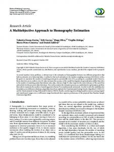
All DERs were modeled as ideal current source considering their devised current control fast enough to track any sinusoidal reference signal. The network power line impedances are shown in Table III. A. Simulation Results It was simulated a daily period where the weights of the decision-making algorithm (i.e, VIKOR method) were varied according to Table IV. Where the greater the weight is, the greater its relevance during the decision is, and then more biased the result will be toward this weight. The selected points in the Pareto-optimal front for the weights used in decision-making method are shown in Fig. 2. The selected individual 1 corresponds to zero power unbalance at PCC, whereas selected individual 3 corresponds to maximum power generation from distributed units. Lastly, selected individual 2 represents a good compromise between these two factors. To evaluate the flexibility of control power generation and power unbalance, Fig. 3, Fig. 4 and Table V show the simulation results. In the basis of Table IV and Fig. 2, in the interval from 0 to 6h, the algorithm tracks the endpoint (selected individual 1) as the point closest to the ideal point, at which point the FG is FG = 0.57, and FNa is your best value FNa = 0.02. In interval from 6 to 9h, the algorithm finds the midpoint (selected individual 2) as the point closest to the ideal point, at which point the FG = 0.71 and the FNa is a medium value FNa = 0.32. In interval from 9 to 17 h, the algorithm reaches the bottom end (selected individual 3) as the point closest to the ideal point. At this point the FG has its maximum value FG = 1, and the FNa has its highest value FNa = 0.52. Finally, in the interval from 17 to 24h, the algorithm selects again the midpoint (selected individual 2). The negative value of FG in Fig 2 is because it is an inherent maximization function, and when it is converted to a minimization function it must be multiplied by “-1”. The result that provides the lower value of FNa is between 0 to 6h, it is possible to see in Fig. 3 the small voltage asymmetry FD < 0.003%, and FNa < 0.02. On the other hand, FG = 0.57, because DERs had to reduce their generation. As expected, in the period from 9 to 17h, the FG remains at its maximum value, FG = 1, and FD increased due to the injection of unbalanced powers from single-phase DERs, FD = 0.38%. Note the effect of unbalance power generation (Fig. 4) at the PCC voltages (Fig. 3). TABLE III Parameters of the three-phase four-wire low-voltage network Line impedances Z[mΩ] From To

N0 N1 N2

N1 N2 N3

460 + j1850 32 + j11.72 20.6 + j7.53

During interval from 6 to 9h and 17 to 24h the factors FG and FD have medium values when compared to the previous cases. Observing the behavior of the voltage at the PCC, the FD is about 0.11%, while the FG is equal to 0.71. Table V summaries the results of all intervals of operation. In Fig. 4 the PCC active power shown. The active power level corresponds directly to the FG of each simulation moment. It is important to emphasize that the small difference (about 2.8%, 3.83% and 4.4% in phases a, b and c) is related to the losses in the network, and the negative value of powers is related to the direction of PCC power flow (DERs to main grid). Oscillations in the power flow are observed during the periods from 6 to 9 and 17 to 24 h. These oscillations happened because VIKOR method selects the final point (Selected individual 1) in some cycles due to variations in the Pareto-Optimal front approach generated by NSGA-II, and a low sensibility in VIKOR method gains. VI. CONCLUSIONS The paper presented an optimal algorithm applied to hierarchical control of centralized networks. By means of the analyses based on quantifying factors FG, FD, FNa and power flow at PCC, it was possible to evaluate the relevance of the multiobjective optimization technique dealing with conflicting objective functions. The proposed approach is a flexible control method that enables maximize the power generation from single-phase distributed units, maintaining controllability over the power unbalance, and consequently voltage asymmetry, without any knowledge of the power line impedances of network. Future works will cope with the control of reactive power, and study other optimization methods that have reduced computational complexity. It may be interesting to apply the proposed method to distributed generators endowed with energy storage capability, as it may increase even more the flexibility in the operation of a microgrid.

Fig. 2. Framework of the estimate Pareto-Optimal front.

Results TABLE IV Weights of the objective functions Simulation Time (h) Weights 0 ~ 6h 6 ~ 9h 9 ~ 17h 1 W1 (FG) 0 0.5 W2 (FNa) 1 0.5 0

17 ~ 24h 0.5 0.5

FG FNa FD (%) VA (V) VB (V) VC (V)

TABLE V Simulation results Simulation Time (h) 0 ~ 6h 6 ~ 9h 9 ~ 17h 1 0.57 0.71 0.02 0.32 0.52 0.003 0.11 0.38 127.6 127.6 127.6 127.6 127.8 128.0 127.6 127.8 128.3

17 ~ 24h 0.71 0.32 0.11 127.6 127.8 127.8

VPCC(V)

PPCC(kW)

Fig. 3. Power quality factors at the PCC. From top to bottom: phase voltage (V), factor of voltage asymmetry (FD), factor of generation (FG), and factor of active unbalance (FNa).

Fig. 4. Active power flow through the PCC.

ACKNOWLEDGEMENT This research was financially supported by CAPES, CNPq (grant 420850/2016-3), FAPESP (grant 2016/08645-9) and Research Council of Norway (grant 261735/H30).

[8]

[9]

REFERENCES [1]

[2]

[3]

[4]

[5]

[6]

[7]

V. N. Coelho, M. W. Cohen, I. M. Coelho, N. Liu and F. G. Guimarães, “Multi-agent systems applied for energy systems integration: Stateofthe-art applications and trends in microgrids,” ELSEVIER Journal of Applied Energy, vol. 187, n°1, pp. 820-832, Feb. 2017. D. I. Brandao, J. A. Pomilio, T. Caldognetto, S. Buso, and P. Tenti, “Coordinated Control of Distributed Generators in Meshed LowVoltage Microgrids: Power Flow Control and Voltage Regulation,” International Conference on Harmonics and Quality of Power (ICHQP), pp. 249-254, Oct. 2016. D. I. Brandao et al., “Centralized Control of Distributed Single-Phase Inverters Arbitrarily Connected to Three-Phase Four-Wire Microgrids,” IEEE Transactions on Smart Grid, vol. 8, n° 1, pp. 437-446, June 2016. T. Caldognetto and P. Tenti, “Integration and Control of Heterogeneous Power Sources in Meshed Distribution Grids,” International Symposium on Power Electronics for Distributed Generation Systems (PEDG), June 2016. S. Weckx, C. Gonzalez and J. Driesen, "Combined Central and Local Active and Reactive Power Control of PV Inverters," IEEE Transactions on Sustainable Energy, vol. 5, n° 3, pp. 776-784, June 2014. A. G. Tsikalakis and N. D. Hatziargyriou, “Centralized control for optimizing microgrids operation,” 2011 IEEE Power and Energy Society General Meeting, Detroit, MI, Jul., 2011. P. Tian, X. Xiao, K. Wang and R. Ding, “A hierarchical energy management system based on hierarchical optimization for microgrid community economic operation,” IEEE Transactions on Smart Grid, vol. 7, n° 5, p. 2230-2241, Sept. 2016.

[10]

[11]

[12]

[13]

[14]

[15]

[16]

[17]

M. Farivar, R. Neal, C. Clarke and S. Low, “Optimal inverter VAR control in distribution systems with high PV penetration,” Power and Energy Society General Meeting, 2012 IEEE, San Diego, CA, Jul., 2012. T. Caldognetto, S. Buso, P. Tenti, and D. I. Brandao, “Power-Based Control of Low-Voltage Microgrids,” IEEE Journal of Emerging and Selected Topics in Power Electronics, vol. 3, n° 4, pp. 1056–1066, Dec. 2015. A. Bidram and A. Davoudi, "Hierarchical structure of microgrids control system," IEEE Transactions on Smart Grid, vol. 3, no. 4, pp. 1963-1976, Dec. 2012. S. Opricovic, “Multicriteria Optimization of Civil Engineering Systems,” Ph.D. Dissertation, Faculty of Civil Engineering, Belgrade, Serbia, 1998. K. Deb, A. Pratap and S. Agarwal, “A Fast and Elitist Multiobjective Genetic Algorithm: NSGA–II,” IEEE Transactions on Evolutionary Computation, vol. 6, n° 2, pp. 182–197, Apr. 2002. R. O. Parreiras, “Algoritmos Evolucionários e Técnicas de Tomada de Decisão em Análise Multicritério,” Ph.D. Dissertation, GPEE, UFMG, Belo Horizonte, BRA, 2006. S. Opricovic and G. H. Tzeng, “Compromise Solution by MCDM Methods: A Comparative Analysis of VIKOR and TOPSIS,” European Journal of Operational Research, vol. 156, n° 2, pp. 445-455, July 2004. D. I. Brandao, H. Guillardi, H. K. M. Paredes, F. P. Marafao and J. A. Pomilio. “Optimized Compensation of Unwanted Current Terms by AC Power Converters Under Generic Voltage Conditions,” IEEE Transactions on Industrial Electronics, vol. 63, n° 12, pp. 7743-7753, July 2016. P. Tenti, H. K. M. Paredes, and P. Mattavelli, "Conservative Power Theory, a Framework to Approach Control and Accountability Issues in Smart Microgrids," IEEE Transactions on Power Electronics, vol. 26, n° 3, pp. 664-673, Mar. 2011. Procedures for Distribution of Electric Energy in the National Electric System (PRODIST), National Electric Energy Agency (ANEEL) Standard Module 8: Energy Quality, 2016. (in Portuguese).