In [10] and in related work, both theoretical and practical [1, 7, 12, 14] it has been ... argminx∈Xf(x). (1). Multiobjectivization by decomposition reformulates the problem through the .... In this section, we consider functions f : {0, 1}n → R2 (with restrictions on n for some .... Left: Part of the function for (x ∈ {1i0n−i,i ∈ 1..n}) for.
Multiobjectivization by decomposition of scalar cost functions Julia Handl, Simon C. Lovell, and Joshua Knowles The University of Manchester, UK {j.handl,simon.lovell,j.knowles}@manchester.ac.uk
Abstract. The term ‘multiobjectivization’ refers to the casting of a single-objective optimization problem as a multiobjective one, a transformation that can be achieved by the addition of supplementary objectives or by the decomposition of the original objective function. In this paper, we analyze how multiobjectivization by decomposition changes the fitness landscape of a given problem and affects search. We find that decomposition has only one possible effect: to introduce plateaus of incomparable solutions. Consequently, multiobjective hillclimbers using no archive ‘see’ a smaller (or at most equal) number of local optima on a transformed problem compared to hillclimbers on the original problem. When archived multiobjective hillclimbers are considered this effect may partly be reversed. Running time analyses conducted on four example functions demonstrate the (positive and negative) influence that both the multiobjectivization itself, and the use vs. non-use of an archive, can have on the performance of simple hillclimbers. In each case an exponential/polynomial divide is revealed.
1 Introduction The term ‘multiobjectivization’ was introduced in [10] to refer to the reformulation of originally single-objective problems as multiobjective ones. Two approaches to this reformulation can be taken, namely the decomposition of the original objective, or the addition of new objectives. In both of these cases, it is a requirement that each of the original optima becomes a Pareto optimum under the new set of objectives [10]. In [10] and in related work, both theoretical and practical [1, 7, 12, 14] it has been demonstrated that such reformulations of problems can in some cases lead to accelerated search performance (comparing broadly equivalent single-objective and multiobjective algorithms). Brockhoff et al. recently presented general theoretical results for adding objectives to a problem, showing that it may have beneficial or detrimental effects on the runtime for a given problem [1]. They show (ibid.) that the addition of objectives to an originally single-objective problem has only two effects on solution orderings: (a) solution pairs that are equal (‘indifferent’) with regard to the single-objective formulation may become comparable (i.e., one dominates the other), or alternatively, (b) solution pairs that are comparable with regard to the single-objective formulation may become incomparable (i.e., neither dominates the other). Running time analyses (ibid.) comparing a (1+1)-EA and the Global SEMO (Global Simple Evolutionary Multi-objective Optimizer) algorithm indicated that large performance differences
2
Multiobjectivization by decomposition
(a polynomial speedup and an exponential slowdown) can be observed for a singleobjective short path function (derived from SPCn [6]) when objectives are added. Here, we are interested in multiobjectivization through decomposition of a singleobjective function, which has not been addressed in [1]. After the introduction of some basic notation and algorithms in Section 2, Section 3 goes on to show that the number of possible effects of a decomposition is in fact reduced compared to the scenario discussed in [1], and that this allows for additional inferences regarding the changes to the fitness landscape. It also discusses why these theoretical results only directly apply to algorithms that do not employ an archive. Section 4 of the paper introduces four example problems: the first two illustrate that, despite the theoretical differences to the scenario considered in [1], multiobjectivization through decomposition can equally render a problem easier or harder. The last two are examples of problems where the introduction of an archive makes the problem significantly easier or more difficult. Finally, Section 5 concludes.
2 Notation and algorithms Formally, an unconstrained single-objective (scalar) optimization problem is described by the set of feasible solutions X and an objective function f : X → R. Without loss of generality, we assume minimization of f , so that the optimal solutions to the problem are those that satisfy argminx∈X f (x). (1) Multiobjectivization by decomposition reformulates the problem through the decomposition of the original objective into two or more components. This is achieved through the definition of k objectives fi : X → R, i ∈ 1..k, with the constraint that f (x) = Pk i=1 fi (x), ∀x. This transforms the scalar optimization problem into a vector optimization problem with every solution x ∈ X mapping to a k-tuple of objective values f (x) = (f1 (x), . . . , fk (x))T . The optimal solutions to the problem are those that satisfy argminx∈X f (x). (2) In vector optimization problems such as (2), a partial ordering of the solutions can be obtained using the concept of Pareto dominance. Solution x is said to dominate solution y, denoted as f (x) ≺ f (y), iff ∀i ∈ 1..k : fi (x) ≤ fi (y) ∧ ∃j ∈ 1..k : fj (x) < fj (y). The solutions x and y are said to be indifferent, denoted as f (x) = f (y), iff ∀i ∈ 1..k : fi (x) = fi (y). Iff x and y are not indifferent and neither dominates the other, they are said to be incomparable or mutually non-dominated, denoted as f (x) ∼ f (y). Under the Pareto framework, the solution to a vector optimization problem is the set of solutions S ⊆ X, which are not dominated by any other solutions in the search space: S = {s ∈ X | 6∃x ∈ X : f (x) ≺ f (s)}. The set of optimal solutions for (1) form a subset of the set of Pareto optimal solutions for formulation (2). Problem (2) can therefore be employed as an alternative formulation to find solutions to (1). Hillclimbers The optimizers considered in this paper are very basic single-objective and multiobjective hillclimbers, defined thus:
Multiobjectivization by decomposition
3
SOHC: Initialize a current solution at random. While not done {mutate the current solution and accept the mutant iff it is not worse than the current } . MOHC: Initialize a current solution at random. While not done {mutate the current solution and accept the mutant iff it is not dominated by the current } . MOHC+A: Initialize a current solution at random and copy it into the nondominated solutions archive. While not done {mutate the current solution and accept the mutant iff it is not dominated by anything in the archive. If the mutant is accepted, copy it to the archive. Remove from the archive any solutions that are dominated} . The mutation operator used in all three algorithms is 1/n bit flip mutation, where n is problem size. The single-objective hillclimber (SOHC) accepts moves to equal cost solutions (cf. [6, 2, 8]). Equivalently, the basic multiobjective hillclimber (MOHC) rejects the mutant solution only if its objective vector is dominated by the parent solution; it accepts moves to incomparable solutions. For the archiving multiobjective hillclimber (MOHC+A), a mutant solution is accepted only if it is not dominated by either the current solution or a solution in the nondominated solutions archive (similarly to (1+1)PAES [11]). As discussed in [9] (pages 102–105), this way of using an archive yields a negative efficiency preserving strategy [5], i.e., it prevents degradation of solutions. We say there is degradation if the current solution is replaced at some later iteration by one that it dominates. Such degradation prevents convergence and can lead to endless cycling between solutions that are not mutually incomparable. N.B., the type of archiving used in the GSEMO algorithm [1] is different because the archive is used as a population from which to select solutions; we do not consider this type of archiving here.
3 Changes to the fitness landscape This section studies the changes in the fitness landscape when moving from a scalar optimization problem to the multiobjective problem obtained through a decomposition of the fitness function as defined in Equation 2. Definition 1 (Neighborhood) We define a neighborhood function as a function ν : X → X m , with the two properties, x ∈ ν(x), and x ∈ ν(y) ↔ y ∈ ν(x). Solutions x and y are said to be neighbors if x ∈ ν(y) (and, equivalently, y ∈ ν(x)). The neighborhood size is m. Definition 2 (Connected sets) A set of solutions S is said to be connected, if ∀s, t ∈ l−1 S : ∃pi ∈ S : p1 = s ∧ pl = t ∧ ∀i=1 pi+1 ∈ ν(pi ). Definition 3 (Local optima) A set of connected solutions S is said to be locally optimal under objective f and neighborhood function ν, iff ∀s ∈ S : ∀t ∈ ν(s) : f (s) < f (t) ∨ (t ∈ S ∧ f (s) = f (t)). Equivalently, a set of connected solutions S is said to be locally optimal under the set of objectives f and neighborhood function ν, iff ∀s ∈ S : ∀t ∈ ν(s) : f (s) ≺ f (t) ∨ (t ∈ S ∧ (f (s) = f (t) ∨ f (s) ∼ f (t)). Every such set S is defined as one local optimum.
4
Multiobjectivization by decomposition
Definition 4 (Plateaus) A set of connected solutions S is said to form a plateau under objective f and neighborhood function ν, iff ∀s ∈ S : ∀t ∈ S : ∃pi ∈ S : p1 = l−1 s ∧ pl = t ∧ ∀i=1 (pi+1 ∈ ν(pi ) ∧ f (pi+1 ) = f (pi )). Equivalently, a set of connected solutions S is said to form a plateau under objective f and neighborhood function ν, l−1 iff ∀s ∈ S : ∀t ∈ S : ∃pi ∈ S : p1 = s ∧ pl = t ∧ ∀i=1 (pi+1 ∈ ν(pi ) ∧ (f (pi+1 ) ∼ f (pi ) ∨ f (pi+1 ) = f (pi ))). A plateau is maximally sized iff 6∃s ∈ {X \ S} such that s ∪ S is a plateau. Theorem 1 (Gradient cannot be introduced). If f (x) = f (y) then f (x) ∼ f (y) ∨ f (x) = f (y). Proof. Assume that f (x) = f (y) and f (x) ≺ f (y). Then, by definition of dominance, for each component of f , fi (x) ≤ fi (y) and there exists a component fj where fj (x) < fj (y). As f (x) = f1 (x) + f2 (x) + . . . + fk (x), this contradicts the assumption that f (x) = f (y). Thus, if f (x) = f (y), then x does not dominate y. By a symmetric argument, y does not dominate x either. Therefore, by definition of the dominance relations, either x and y are indifferent (the same in all components) or incomparable. ⊓ ⊔ Theorem 2 (Gradient cannot be reversed). If f (x) ≺ f (y) then f (x) < f (y). Proof. Assume that f (x) ≺ f (y). Then, by definition of dominance, the objective value of x will be smaller than that of y under f , which, by definition, is the sum of the components of f . ⊓ ⊔ The implication of Theorem 1 and 2 is that decomposition of a scalar cost function has a single consequence for solution orderings: to introduce plateaus. We next prove that multiobjectivization by decomposition decreases or leaves unchanged the number of local optima in a landscape. We first show that our definition of local optimum ensures that local optima are disjoint sets. This is sufficient to ensure that their number is well-defined. This holds in both the single-objective and the multiobjective spaces. We then show that for each optimum in the multiobjective space there is at least one in the single-objective space. Taken together with the fact that local optima are disjoint, this is sufficient to prove the theorem. Lemma 1. The local optima are uniquely defined and are disjoint sets (both in the single-objective and the multiobjective space). Proof. The definitions of the local optima above ensure that each one is a maximally sized set and all immediate neighbors of the set are worse. Two local optima cannot contain the same solution because this would necessitate them being in the same optimum; hence the sets are disjoint and uniquely defined. ⊓ ⊔ Lemma 2. A locally optimal set in the multiobjective landscape contains at least one locally optimal set in the single-objective landscape. Proof. Let S be a set of connected solutions that is locally optimal under f . Then, we know that ∀s ∈ S : ∀t ∈ ν(s) : f (s) ≺ f (t) ∨ (t ∈ S ∧ (f (s) = f (t) ∨ f (s) ∼ f (t)). If t is not part of S, it follows that s dominates t and, by Theorem 1 and 2, the gradient
Multiobjectivization by decomposition
5
between s and t remains under the single-objective formulation: ∀s ∈ S : ∀t ∈ ν(s) : f (s) < f (t) ∨ t ∈ S. The set S is then split into the following sets: S ∗ = mins∈S f (s) and T ∗ = S \ S ∗ . By definition, we know that ∀s ∈ S ∗ : ∀t ∈ T ∗ : f (s) < f (t). It follows that ∀s ∈ S ∗ : ∀t ∈ ν(s) : f (s) < f (t) ∨ (t ∈ S ∗ ∧ (f (s) = f (t))). The set S ∗ may consist of one or more sets of connected solutions, each of which corresponds to one local optimum (additional optima on different fitness levels are also possible). ⊓ ⊔ Theorem 3. The number of local optima under f is smaller or equal to the number of local optima under f . Proof. The result follows directly from the two previous lemmata.
⊓ ⊔
How does this affect search? An increase in the number and size of plateaus may contribute to making a problem more difficult, as, on such plateaus, optimization methods have to succumb to random walk behavior. On the other hand, a reduction in the number of local optima may mitigate the difficulty of search. Both effects are intimately linked, as the removal of local optima is only possible through the creation of a plateau: it requires the creation of at least one path of incomparable solutions that crosses the fitness barrier around the original local optimum. Whether a problem gets easier or more difficult as a result of the decomposition will thus depend on the number and size of the plateaus that are created and the parts of the fitness landscape they replace. In Section 4.1. and 4.2., we introduce two examples of decompositions that cause an exponential increase or decrease in the runtime required by a multiobjective hillclimber compared to the runtime required by a single-objective hillclimber on the corresponding singleobjective problem. What about archives? The introduction of an archive (of the type used in MOHC+A) has the effect of restricting movement along plateaus of incomparable solutions, dependent upon what solutions are in the archive. On one hand, this means that, from the point of view of the algorithm, some of the local optima removed by the decomposition may again be perceived. On the other hand, degrading moves are prevented, which may have a beneficial effect on search. In Section 4.3. and 4.4., we introduce functions that are examples of problems where the introduction of an archive makes a multiobjective function (alternately) harder or easier.
4 Four example functions In this section, we consider functions f : {0, 1}n → R2 (with restrictions on n for some problems), each being a decomposition of a different single objective function f . In our discussion of these functions, we consider local optima as defined by the neighborhood function ν(x) = {y|H(x, y) ≤P 1}, where H(x, y) is the Hamming distance of two bit strings defined as H(x, y) = ni=1 |xi − yi |. We provide proof sketches1 regarding the derivation of theoretical bounds on the runtime required by the different algorithms to reach the global optimum and give empirical results on the number of evaluations taken (means and standard errors over 20 runs; their approximate fitting with analytical curves agreeing with the theoretical bounds on time complexity is also shown). 1
Proof details can be obtained from the first author.
6
Multiobjectivization by decomposition
4.1 Decomposition can make a problem harder We define the function slope(x) = (f1 (x), f2 (x))T over the set of binary strings x ∈ {0, 1}n: f1 (x) = |x|1
f2 (x) = 2n − 2|x|1 ,
where |x|1 gives the number of ones in binary string x. The effect of multiobjectivization in this example is the generation of a plateau of exponential size. A plot of the function and empirical results are given in Figure 1.
40
1e+07
f1 f2 f1 + f2
35 30
100000
3
10000
3
Evals
3 3
1000
15
+ +
+
+ + + + + + + + + + + + + + + +
3+
10
5 0
3
100
10
3 +
3
25
Fitness20
MOHC SOHCn 2 2.5n log n
3 3
1e+06
3
1
0
5
10
15
20
0
|x|1
10
20
30
40
50
60
70
80
90
100
Problem Size, n
Fig. 1. Function slope(x). Left: Function for n = 20. Right: Empirical results.
We consider the runtime required by SOHC and MOHC to reach the global optimum of f1 (x) + f2 (x) at |x|1 = n. SOHC reaches this optimum by hillclimbing (descending) the monotonic slope towards it. The expected runtime for the problem is equivalent to that of MAXONES, which is Θ(n log n) [6]. For MOHC every solution is incomparable with respect to every other. Therefore, the expected waiting time for MOHC is equivalent to that of the (1+1)-EA on the needle-in-a-haystack function, and is given as Θ(2n ) [3]. MOHC+A performs identically to MOHC, as degradation of solutions cannot occur for this problem. 4.2 Decomposition can make a problem easier The function we use here is inspired by the short path function defined in [6], which was used as a basis for some other functions in [1]. We define the function shortpath(x) = (f1 (x), f2 (x))T over the set of binary strings x ∈ {0, 1}n: if x ∈ {1i 0n−i , i ∈ 1..n} ∧ |x|1 ≤ n − 1 2|x|1 if x ∈ {1i 0n−i , i ∈ 1..n} ∧ |x|1 = n f1 = 0 2n + |x|1 otherwise, � n − |x|1 if x ∈ {1i 0n−i , i ∈ 1..n} f2 = 2n + |x|1 otherwise.
Multiobjectivization by decomposition 40
1e+09
f1 f2 f1 + f2
35
7
MOHC SOHC n3 nn
1e+08
30
1e+07
25
1e+06
Fitness20
Evals
1e+05
3 3 3
+
15
10000
10
1000
5
100
0
+
3 3
3 +
3 3 3 3 3 3 3 3 3
3 3 3 3 3
+ 3
10 0
5
10
15
20
|x|1
0
10
20
30
40
50
60
70
80
90
100
Problem Size, n
Fig. 2. Function shortpath(x). Left: Part of the function for (x ∈ {1i 0n−i , i ∈ 1..n}) for n = 20. Right: Empirical results.
The effect of multiobjectivization is the introduction of a plateau that is a short path and the removal of the local optimum at |x|1 = 0. A plot of this crucial part of the function and empirical results are given in Figure 2. We consider the runtime required by SOHC and MOHC to reach the global optimum of f1 (x) + f2 (x) at |x|1 = n. MOHC behaves equivalently to the (1+1)-EA on function SPCn [6] and its expected runtime is therefore bounded by O(n3 ). MOHC+A performs identically to MOHC, as degradation of solutions cannot occur for this problem.2 Regarding the expected runtime of SOHC, a lower bound of nΩ(n) can be shown similarly to the analysis of the (1+1)-EA on SPCn in [6]. 4.3 An archive can make a problem harder We define the function barrier(x) = (f1 (x), f2 (x))T over the set of binary strings x ∈ {0, 1}n for n mod 10 = 0: � n − |x|1 if|x|1 ≤ 0.9n − 2 f1 (x) = 1.1n − |x|1 + 2 otherwise, � n − |x|1 if|x|1 ≤ 0.9n − 1 f2 (x) = 1.1n − |x|1 + 1 otherwise. The effect of the use of an archive is to make parts of a plateau inaccessible. A plot of the function and empirical results are given in Figure 3. We consider the runtime required by MOHC and MOHC+A to reach the global optimum of f1 (x) + f2 (x) at |x|1 = n. Function barrier(x) has a plateau of incomparable solutions at 0.9n − 2 ≤ |x|1 ≤ 0.9n. With probability exponentially close to 1, the hillclimbers are initialized with a solution with |x|1 < 0.9n − 2 (this follows by Chernoff’s bounds, see [4, 6]), and will need to cross the plateau to reach |x|1 = n. 2
The possibility of degradation can be readily introduced into a function of the same structure through the adjustment of relative fitness levels between solutions that lie within and outside of x ∈ {1i 0n−i , i ∈ 1..n}, so that MOHC can fall off the short path. In that case, MOHC+A will outperform MOHC.
8
Multiobjectivization by decomposition 40
1e+25
f1 f2 f1 + f2
35
MOHC+A MOHC 10n(0.1n+1) 2000nlog(n)
1e+20
30 25
1e+15
Fitness20
Evals 1e+10
15 10
100000
5 0
3 +
3 +
3 +
+
30
40
+
+
+
+
+
+
50
60
70
80
90
100
3 + 1
0
5
10
15
20
|x|1
10
20
Problem Size, n
Fig. 3. Function barrier(x). Left: Function for n = 20. Right: Empirical results.
MOHC will reach the plateau in expected time Θ (n log n). It will then perform a random walk on the plateau until it succeeds in adding at least three more ones to the bit string. A lower bound on the probability of this success can be obtained as the probability of performing three drift moves to the right directly in sequence, which is given Q0.1n+2 k n−1 (n−1) as k=0.1n . The waiting time for this event is O (1). Once the plateau n( n ) has been crossed, any mutation that � |x|1 will be accepted, and the probability � increases n−|x|1 . If only such mutations were possible, the of such a mutation is at least Ω n
expected waiting time for reaching the global optimum would be O (n log n). However, mutations reducing |x|1 to 0.9n − 2 ≤ |x|1 ≤ 0.9n − 1 can also be accepted: these require� at least k = |x|1 − 0.9n + 1 simultaneous bit flips and have probability at most 1 . At position |x|1 , a lower bound on the probability of an increase in |x|1 to hapO k! pen before a decrease in |x|1 is then given as pk = k!+ k! n . Multiplying over all 0.1n−k+1 Q0.1n 0.9n + 1 ≤ |x|1 ≤ n − 1 yields k=2 pk , which converges. Therefore, the possible returns to the plateau only increase the expected waiting time by a constant factor, and the overall expected runtime of MOHC is O (n log n). MOHC+A will reach the plateau in expected time Θ(n log n). The archive then prevents the access of all the solutions with 0.9n ≤ |x|1 ≤ n − 1. In order to reach the global optimum at |x|1 = n, it will need to set all remaining 0.1n + 1 or 0.1n + 2 bits with value zero to one simultaneously. The probability of such a mutation is bounded above by O (( n1 )(0.1n+1) ). The lower bound on the overall runtime of the MOHC+A is therefore given as nΩ(n) . 4.4 An archive can make a problem easier We define the function steps(x) = (f1 (x), f2 (x))T over the set of binary strings of even size: x ∈ {0, 1}n for n mod 2 = 0. f1 (x) =
�
0.5n − 0.5|x|1 if|x|1 mod 2 = 0 0.5n − 0.5|x|1 + 1 otherwise,
f2 (x) =
�
0.5n − 0.5|x|1 if|x|1 mod 2 = 0 0.5n − 0.5|x|1 − 2 otherwise.
Multiobjectivization by decomposition
9
The effect of the use of an archive is to prevent degradation on this plateau of neighboring non-dominated solutions. A plot of the function and empirical results are given in Figure 4. 20
1e+08
f1 f2 f1 + f2
15
MOHC+A MOHC π 2 /6 × n2 20.8n
1e+07
3 +
1e+06
10
+
100000
Fitness
Evals 10000
5
+
1000
+
0
3
3 3
3
3 3
3 3 3 3 3 3 3 3 3 3 3 3
3
100 + 3
-5
10
0
5
10
|x|1
15
20
0
10
20
30
40
50
60
70
80
90
100
Problem Size, n
Fig. 4. Left: Function steps(x) for n = 20. Right: Empirical results.
We consider the runtime required by MOHC and MOHC+A to reach the global optimum of f1 (x) + f2 (x) at |x|1 = n. In order to reach |x|1 = n, MOHC+A needs to increase the number of ones and drift through the plateaus that separate it from the global optimum. Alternatively, it can overcome each such plateau by two simultaneous mutations and, at position |x|1 , the probability of increasing the number of ones by � 1 2 n−1 n−2 1 two is therefore bounded below by n−|x| (n) ( n ) . Summing over all values 2 2 of |x| then yields an upper bound of (n ) on the expected runtime of MOHC+A (as O Pn 1 1 converges). |x|1 =0 |x|21 In contrast to this, MOHC may drift back to |x|1 = 0 from any point in the search space (using single bit flip mutations). In order to show exponential runtime we make use of the drift theorem introduced by Oliveto and Witt [13]. Let △(i) denote the random increase in the number of zeros when mutating a bit string with |x|1 = i. We now need to identify an interval [a, b] of asymptotic size on 0 ≤ |x|1 ≤ n for 1 j−r which it can be shown that (1) P (△(i) = −j) ≤ 1+δ for i > a and j ≥ 1 and (2) E(△(i)) > ǫ, for a < i < b, where δ, r and ǫ are constants. As shown in [13], Condition 1 holds for the (1+1)-EA independently of i and of acceptance, which also carries over to our analysis. For a = 32 n and b = n, it can be shown that E (△(i)) > 61 e−1 , for a < i < b, which fulfills Condition 2. It follows that the probability of finding the global optimum in 2cn steps is at most 2− Ω(n) .
5 Conclusion This paper has considered the transformation of scalar optimization problems into multiobjective ones. Where the multiobjective problem is obtained through a decomposition of the original objective function, this can cause only one type of change to solution orderings: pairs of solutions that initially had different scalar objective values can become incomparable. Running time analyses and empirical results for both archiving and non-archiving algorithms show that, dependent on the function, a problem can become
10
Multiobjectivization by decomposition
easier or harder. This can be understood in terms of the introduction and removal of plateaus and local optima.
Acknowledgments We thank the anonymous reviewers for their many helpful comments and advice. JH gratefully acknowledges support by a Special Training Fellowship from the Medical Research Council (MRC), UK. JK is supported by a David Phillips Fellowship from the Biotechnology and Biological Sciences Research Council (BBSRC), UK
References 1. D. Brockhoff, T. Friedrich, N. Hebbinghaus, C. Klein, F. Neumann, and E. Zitzler. Do additional objectives make a problem harder? In Proceedings of the 9th Annual Conference on Genetic and Evolutionary Computation, pages 765–772. ACM Press, New York, NY, 2007. 2. S. Forrest, M. Mitchell, and L. Whitley. Relative Building-Block Fitness and the BuildingBlock Hypothesis. In Foundations of Genetic Algorithms 2, pages 109–126. Morgan Kaufmann, San Mateo, CA, 1993. 3. J. Garnier, L. Kallel, and M. Schoenauer. Rigorous hitting times for binary mutations. Evolutionary Computation, 7(2):173–203, 1999. 4. T. Hagerub and C. R¨ub. A guided tour of Chernoff bounds. Information Processing Letters, 33:305–308, 1989. 5. T. Hanne. On the convergence of multiobjective evolutionary algorithms. European Journal of Operational Research, 117(3):553–564, 1999. 6. T. Jansen and I. Wegener. Evolutionary algorithms — how to cope with plateaus of constant fitness and when to reject strings of the same fitness. IEEE Transactions on Evolutionary Computation, 5(6):589–599, 2001. 7. M. T. Jensen. Helper-objectives: Using multi-objective evolutionary algorithms for singleobjective optimisation. Journal of Mathematical Modelling and Algorithms, 3(4):323–347, 2004. 8. A. Juels and M. Wattenberg. Stochastic Hillclimbing as a Baseline Method for Evaluating Genetic Algorithms. In D. S. Touretzky, editor, Advances in Neural Information Processing Systems 8, pages 430–436. MIT Press, Cambridge, MA, 1995. 9. J. Knowles. Local-search and hybrid evolutionary algorithms for Pareto optimization. PhD thesis, University of Reading, UK, 2002. 10. J. Knowles, R. Watson, and D. Corne. Reducing local optima in single-objective problems by multi-objectivization. In Proceedings of the First International Conference on Evolutionary Multi-Criterion Optimization, pages 269–283. Springer-Verlag, Berlin, Germany, 2001. 11. J. D. Knowles and D. W. Corne. Approximating the nondominated front using the Pareto archived evolution strategy. Evolutionary Computation, 8(2):149–172, 2000. 12. F. Neumann and I. Wegener. Minimum spanning trees made easier via multi-objective optimization. Natural Computing, 5(3):305–319, 2006. 13. P. S. Oliveto and C. Witt. Simplified drift analysis for proving lower bounds in evolutionary computation. In Proceedings of the Eight International Conference on Parallel Problem Solving from Nature. Springer-Verlag, Berlin, Germany, 2008. 14. J. Scharnow, K. Tinnefeld, and I. Wegener. The analysis of evolutionary algorithms on sorting and shortest paths problems. Journal of Mathematical Modelling and Algorithms, 3(4):346–366, 2004.