SCOGS,26 a Gauss-Newton program. ..... Gauss-Newton iteration on some âguessedâ concen- ...... L. G. Sill&n and B. Wamqvist, Ark. Kemi, 1968, 31, 377. 7.
0039-9140/86 53.00+0.00
Tdanfa,Vol.33,No. 6,pp. 513-524,1986
Pergamon Journals Ltd
Printed in Great Britain
MULTIPARAMETRIC
CURVE FITTING-X
A STRUCTURAL CLASSIFICATION ANALYSING MULTICOMPONENT USE IN EQUILIBRIUM-MODEL
OF PROGRAMS FOR SPECTRA AND THEIR DETERMINATION
MILAN MELOUN Department of Analytical Chemistry, College of Chemical Technology, CS-532 10 Pardubice, Czechoslovakia MILAN JA~~REK Computing Centre, College of Chemical Technology, CS-532 10 Pardubice, Czechoslovakia
JOSEFHAVEL Department of Analytical Chemistry, Purkyni University, CS-611 37 Bmo, Czechoslovakia (Received 6 February 1985. Revtied 4 Jonuary 1986. Accepted 23 January 1986) Summary-A functional structure-classification of programs for analysis of spectra elucidates their efficiency for determination of the stoichiometric indices, stability constants and molar absorptivities of complex species. SQUAD (84) introduces new functional units for (i) determination of the number of light-absorbing species, (ii) a rigorous fitness test, (iii) plotting three-dimensional graphs of a paraboloid minimum response-surface as a function of two selected parameters, and a graph of the fitted absorbance response-plane, (iv) simultaneous estimation of stoichiometric indices and stability constants, (v) simulation of an absorbance matrix data by loading with random errors related to the instrumental variance of the absorbance. A guide to experimental procedure and computational strategy for chemical model determination is given and nine diagnostic tools useful in finding the number of species present and their stoichiometry and stability constants by regression analysis of spectra are tested, by use of literature data.
The spectrophotometric study of solution equilibria has been greatly advanced by computer-assisted methods of analysing spectra,‘-20 but comparatively few programs are yet available. Programs for calculation of stability constants from spectrophotometric data are usually classified according to the algorithm
used,‘,* but the structural classification introduced earlier in this series)-’ seems to be useful for comparing the number and efficiency of the logic tools used in a program. Splitting a program structure into logic units helps in elucidation of its anatomy and makes further program implementation and modification easier. It also helps in understanding the modus operandi of a rather sophisticated and long program. This paper is intended to familiarize the reader with the individual logic units of sophisticated programs for analysis of multicomponent spectra, and is illustrated with eight selected programs, LETAGROP-SPEF0,6 FA608 + EY608,’ SQUAD(75),8 SQUAD(78),9 DALSFEK,” PSEQUAD,” SQUAD(80)‘2~‘3 and the new SQUAD(84),
the last of which incorporates
new diagnostic tools.
FA608 + EY608 and LETAGROP-SPEFO have been extended to include a fitness test, printerplotting of graphs, etc. A guide to efficient experimentation and computer evaluation for validating chemical models is given, and use of the recommended diagnostics is illustrated by an example.
THEORY
Study of equilibria spectra
by analysis
of multicomponent
In absorbance-data analysis the Lambert-Beer law and the law of absorbance additivity are assumed to hold. The published programs can deal with various numbers, n., of components, ranging from three (metal M, ligand L and proton H) for LETAGROPSPEF06 to five (two metals, two ligands and proton or hydroxide) for SQUAD,‘*‘**” which form a set of species of general formula M,LqH,, a particular chemical model being represented by nE such species and their stoichiometry, (p, q, r)j, j = 1, . . . , n,, the overall stability constants being expressed in the general form &, =
Part IX: Talanta, 1986, 33, 435, 513
~~,~,~,II~~~lP~~19~~l’~ = cl(mPlqW (1)
514
MILAN MELOUN et
For the ith solution measured at the kth wavelength, the absorbance A, is given by Aik =
2
Q~C,
J=’
z
al.
complexes in the equilibrium mixture, (M,L,H,],, j=l,... , n,, forming for II, solutions the matrix C. Structure of the regression program for analysis of spectra
Each logic unit of this advanced regression problock, which may contain one or more subroutine(s), and the diagram where E~~,~ is the molar absorptivity of species in Fig. 1 of reference 5 may therefore be extended M,L,H, at the kth wavelength. The absorbance A* for new units. Eight programs will be compared in is an element of the (n, x n,) absorbance matrix A for Table 1, and their structures discussed. n, solutions with known concentrations cM, cL, and cH The LETAGROP-SPEFO pit-mapping algorithm and at n, wavelengths. The Lambert-Beer law can be by Sill&n and Warnqvist6 was a pioneering program written in matrix notation as for chemical-model determination by analysis of spectrophotometric data, and some of its features are A=& (3) still unsurpassed. Absorbance and concentration data where E is the (n, x n,) matrix of the molar absorpare treated separately for each wavelength to adjust tivities and C is the (n, x n,) matrix of the concenBWr and a,,, and then the computer calculates the trations of the species concerned. It is assumed that minimum residual-square sums, and finds the all n, species absorb light in the chosen spectral range. lowest value for U for a set of parameters bpq,. The The spectrophotometric equilibrium program is set minimization process to find the “best” stability up to adjust &, and ewr for any absorbance data by constants SW, and molar absorptivities is applied at minimizing the residual-square sum function CJ two levels: the /I,, values are varied on the upper level, and for each set of &,, the concentrations and molar absorptivities of the complexes are calculated i=l k-l at the lower level. The sum of squared residuals can be set on input to refer to the absolute residuals or the relative residuals. Negative values of e,,,, are eliminated by subroutine MIKO. Kankare’s regression program FA608 + EY608 where the dependent variable Aik is an element of the evaluates equilibrium constants and their standard (n, x Q) absorbance response-plane, and the independent variables are the total concentrations cM, cL deviations for multicomponent systems, from spectral data.’ The factor analysis algorithm, FA608, and c,, which are varied in the n, solutions. Parameters to be determined may be divided into three estimates the number of independently varying lightgroups according to the approach to be used in the absorbing species and eliminates any “outlying” spectra points. The hypothetical chemical model computation as follows. (1) A hypothetical chemical model is supplied by defined by the stoichiometric coefficients of the reacthe user in the input. This includes a guess for the tion products is tested by searching for optimum number of light-absorbing complexes, n,, and a list of values of the equilibrium constants, molar absorptivities and concentrations of all species of interest by species assumed, or proved by means of an automatic species selector (the trial and error method) to be algorithm EY608. present. Some programs do not require a guess for n, PSEQUAD is an advanced program for analysis of as input [e.g., FA608+EY608,’ SQUAD(78)9 and spectrophotometric and potentiometric data on equiThe SQUAD(84)J; instead, advanced factor analysis is libria, developed by Nagypsil and ZkBny.” used to determine the absorbance matrix rank, which program calculates all unknown free concentrations should be equal to or less than n,. In solutions with of components from the mass-balance equations by an original method, along with stability contants and a limited number of complexes, direct determination of stoichiometric indices (the variable stoichiometric molar absorptivities. DALSFEK, by Alcock et al.,” deals with two types indices method14) is an alternative to guessing which complexes are present. of observable variables, absorbance and the potential (2) The estimates of the stability constants BwrJ, of an indicator electrode, and both are used in the j=l,... program as dependent variables. The total concen, n,, are adjusted by the regression algortrations are assumed to be independent variables. The ithm and at the same time a matrix of molar absorptivities [&,&, k = 1,. . . , n,),, j = 1,. . , n,] is Marquardt methodZS is used to fit free concentrations estimated from the current values of stability of each species to the mass-balance equations. The constants. same algorithm is used to refine the stability con(3) For a set of current values of /3,1 the free stants. SQUAD was developed by Leggett and McBryde’ concentrations of metal m and ligand f, [H+] is known from pH measurement), for each solution in 1975 and is denoted here as SQUAD(75). calculated, and then the concentrations of all the JanEBi and Have19 made some improvements and =
(E,,,kSmrmPlqh’)j
(2) gram represents one functional
515
Multiparametric curve fitting-X
r e E 2 b :: 4
0.664 0.556 0.452 0.346 0.240 0.134
7.v
7
230
250
270
290
310
330
350
370
390
410
430
X (nm)
Fig. 1. Three-dimensional graph of the absorbance-response-plane of 37 experimental spectra at 20 wavelengths for various mole-ratios of 2,3_dihydroxynitrobenzene (LH,) and boric acid (MH), qM= c,/c,, vs. pH. Data taken from ref. 47.
produced SQUAD(78), known in the literature as SQUAD-G,9,‘5*‘6 which can read spectra without a constant wavelength increment. A segmented version of SQUAD(78) can be used with small computers; both versions were extensively tested.9 Leggett” also revised SQUAD(75) to produce SQUAD(80)” which has “user-friendly” data input to simplify its use. The chemical model hypothesis is changed by addition or removal of one card per species, since all information relevant to a species is collected on one card. The molar absorptivitiy computation can be done by multiple regression or constrained non-negative linear least-squares. Meloun”~‘* extended the diagnostic tools in SQUAD(80) for (i) determination of the number of light-absorbing species, (ii) a test for degree-of-fit by statistical analysis of residuals of each spectrum and of the whole absorbance matrix, (iii) a printer-plot of estimated molar absorptivities and their standard deviations vs. wavelength. The result, SQUAD(81), has been tested.2’*22The new version SQUAD(84), contains some additional diagnostics, including a three-dimensional graph of the predicted absorbance response-plane through the experimental points, and of the paraboloid response-surface of the U function as a function of two parametric coordinates. SQUAD(M) also generates simulated spectra on the basis of the selected stability constants, molar absorptivities and experimental conditions of the equilibrium system, and produces an absorbance matrix containing elements loaded with random
error. Stoichiometric indices are determined together with the stability constants of the complexes by the stoichiometry estimation method.i4 Logic units (1) The RESIDUAL-SQUARE
SUM unit.
LETAGROP-SPEF06 allows a choice in the formulation of the residual-square-sum, between “absolute” [equation (4)] and “relative” residuals. The other programs in Table 1 use absolute residuals, and DALSFEK” and PSEQUAD” also allow treatment of potentiometric data. PSEQUAD can minimize a U function composed from volume (or concentration) residuals, potential residuals and absorbance residuals simultaneously, according to the weighting factor for each type of residual selected on input. (2) The MINIMIZATION
unit.
LETAGROP-SPEF06 uses the pit-mapping algorithm24 with “trial-and-error” human-controlled minimization. Kankare’ modified Chandler’s STEPIT in program EY608. DALSFEK’O uses Marquardt’s method25 and PSEQUAD” the Gauss-Newton method. The first version of SQUAD was based on SCOGS,26 a Gauss-Newton program. The latest versions of SQUAD use conventional multiple regression (MR) in the SOLVE subroutine for solving a set of over-determined linear equations. The MR technique is interchangeable with the NNLS (the Gauss-Newton non-negative least-squares algor-
(lh (2), (3), (5), (6), (8), (9), (lo)
12. OUTPUT (print of) (l), (2), (3)> (4)* (5), (8), (9X (10)
(l), (2), (3), (4) (5), (6), (8), (9), (lo), (11)
8. 6, 20, n,
A. 5, 6, 26, 30 B. 5, 10, 50. 70
4, 7, 40, 50
3, 20, 25, 50
11. INPUT (x,, nc, n,, n,)
Missing
Missing
Missing
10. VISUALIZATION
Missing
STYRE block
STEPIT (Algorithmic) Missing
Pit-mapping (Heuristic)
8. ABSORPTIVITY (Process) 9. SPECIES SELECTOR
A. Missing B. RANKANAL Triangularixation ECOEF routine (Algorithmic) Missing
FA608 Factor analysis
Missing
(l), (2), (3), (5), (6), (8), (lo)
(l), (2), (3), (5) (6)> (7), (8), (9), (10)
Dynamic dimensions
E =f(A) curves
‘Third strategy”, (Algorithmic) Species selector
Marquardt (Algorithmic) Missing
Missing
Newton-Raphson
Random error
s(A) s(B,,x &,) re+B, m,,,, IfI
Absorbance, e.m.f., volume Gauss-Newton (Algorithmic)
PSEQUAD
Separate program
Gauss-Newton
Newton-Raphson
STEPIT
BDTV routines
6. FREE CONCENTRATION 7. SPECIES NUMBER
Missing
Missing
5. DATA SIMULATION
A. -- Missing .
A. So, i = 1, n, B. STATS test Missing
A. Missing B. STATS test
4. FITNESS TEST
s(A) s(B,,), s(+,) Pq R-factor
Absorbance, e.m.f. Marquardt (Algorithmic)
DALSFEK
s(A) r(B,)* s(cm,) Pi, s(r),, i = 1, n,
Gauss-Newton (Algorithmic)
STEPIT (Algorithmic)
1. RESIDUAL-SQUARE SUM 2. MINIMIZATION (Process is)
3. ERROR ANALYSIS
Absorbance
Absorbance
Absolute and relative absorbance Pit-mapping (Heuristic)
Logic unit
equilibrium programs for chemical model determination
A. SQUAD( 1975) B. SQUAD(1978)
FA608 + EY608 A. Original B. Extended
Table 1. A survey of advanced spectrophotometric
LETAGROP-SPEFO A. Original B. Extended
(l), (2), (3), (4) (5), (6), (7), (8) (9), (1% (ll), (12)
A. Missing B. A-plane U-plane (I contour 8 =f(A) curves 5, 14, 40, 40
A. Missing B. ES1 method
Constrained Newton-Raphson A. Missing B. FA608 Factor analysis ECOEF routine (Algorithmic)
+(A), s(A) S(B,,)q &,) Pij A. Missing B. STATS test A. Missing __ .
Multiple regression, NNLS Gauss-Newton method (Algorithmic)
Absorbance
A. SQUAD(1980) B. SQUAD(1984)
2
?
Multiparametric curve fitting-X
517
ithm) method which computes molar absorptivities, but is protected against the occurrence of negative elements in the solution vector.
are possible or proposed, and to establish whether or not the chemical model represents the data adequately, the residuals should be analysed.28 The goodness-of-fitness achieved is easily seen by exam(3) The ERROR ANALYSIS unit. ination of the differences between the experimental In LETAGROP-SPEF0,6 as in LETAGROP in and calculated values of the dependent variable, general, there are several statistical measures: the ri,k = Aexp.i.k - Adc,i,k. One of the most important statistics calculated is the standard deviation of the standard deviation of the absorbance, s(A), denoted here as SIGY, is found by dividing iJ,, by the dependent variable, s(A), calculated from the set of number of degrees of freedom; the standard devi- refined parameters at the end of each minimization ations of the stability constants, s(/$), are found by cycle, and when the minimization is terminated. It is usually compared with the standard deviation of defining the “D-boundary” supercurve, and taking absorbance calculated by a factor analysis, sk(A), and the standard deviation s(pi) for each pi parameter as the maximum difference, s(/$) = [(fil, - /Inun).] I max if s(A) < sk(A), or s(A) 0.010 indicates that a good fit has still not lated from U,, in the same way as in LETAGROPbeen obtained. The statistical tools applied to a set of SPEFO. DALSFEK’O calculates in its final iteration residuals have been described.4*29*30 an unbiased estimate of the variance of an obserIf s(A) or the mean residual and its standard vation with unit weighting, and the standard deviation are too large compared with sk(A) and deviations of the parameters, from the variancecovariance matrix. Correlation coefficients are also s+,,(A), respectively, the postulated stoichiometry of the chemical model tested is incorrect, or the mincalculated to allow consideration of the conditioning imization algorithm has found a false minimum. of the problem, and the precision of the parameter Graphical presentation of the residuals assists the estimates. detection of an outlier spectrum point, a trend in the PSEQUAD” evaluates s(A), the standard devispectrum residuals, or an abrupt shift of level in the ations of the parameters, s@), and the partial, spectra. The actual distribution of the spectrum multiple and total correlation coefficients. These are residuals is tested to find out whether it is Gauscalculated from the elements of the matrix B = J’WJ sian,4929by means of the residual mean m,, , the mean where J is the Jacobian matrix, JT is its transpose and residual lrl, and its standard deviation s(r), the W is the diagonal weighting matrix used in the skewness ms3 (should be zero), the curtosis mrT4 Gauss-Newton method. The partial correlation coefficient gives a measure of the interdependence of (should be 3) and the Pearson x2 test. If the Hamilton R-factor of relative fit, expressed as a percentage two parameters /Ii and /Ii with the assumption that the (R x lOO%), is 2% the fit is poor. The R-factor gives a rigorous The total correlation coefficient also give a measure test of the null hypothesis Ho (giving R,) against the of the interdependence of two parameters, but the alternative H, (giving R,). H, can be rejected at the other parameters are regarded as adjustable: CIsignificance-level if RJR,, > &,,,+,,,.), where n is the pii = Cii/CiiCj)‘/‘. The multiple correlation coefficient gives a measure of the independence of a number of experimental points, m is the number of unknown parameters, and (n -m) is the number of given stability constant from all the others, degrees of freedom.‘The value of R,,,_,,,, may be R, = [1 - 1/BiiCii)]“2 where C = B-i. All these corfound in statistical tables.30 relation coefficients may have values between - 1 and Most programs calculate only s(A). EY608 and + 1. Zero means complete independence, and + 1 or LETAGROP-SPEFO calculate s(A) for each spec- 1 means complete correlation. Two completely correlated species cannot be included in a chemical trum; we have extended both to allow statistical model simultaneously, because the relevant stability analysis of residuals by the STATS subroutine.29 constants are strongly correlated. PSEQUAD” calculates m,,, and IP I as well. Rigorous SQUAD estimates s(A), the standard deviations of residuals analysis by the STATS subroutinez9 is included in SQUAD(84). the stability constants, s(/$), and total correlation coefficients. (5) The DATA SIMULATION unit. (4) The FITNESS TEST unit. To test the reliability of program function for a This unit contains the criteria for testing the correctness of a hypothetical chemical model. To identify the “best” or true chemical model when several
particular type of equilibrium, simulated data are often used. For true values of the parameters (stability constants and molar absorptivities) and
518
MILAN MELOUN er al.
given concentrations and pH, “theoretical spectral points” are calculated precisely. Each theoretical point is then transformed into an “experimental” one by the addition of a random error, e, generated by a random-error generator, and related to the instrumental error of absorbance, sinst(A), set by the user on input. These random errors should have Gaussian distribution, but this must be checked as described earlier.4 Loading points with high random errors is likely to cause a decrease in the accuracy and precision of the parametric estimates; the lower the value of Sins,(A), the more accurate and precise are the estimates. When many parameters are to be refined or there are ill-conditioned parameters in a chemical model, spectra of lower precision may result in erroneous and uncertain values of the parametric estimates. Only PSEQUAD,” SQUAD(78)9 and SQUAD(84) allow such data simulation. SQUAD(84) checks the actual distribution of the errors as well. (6) The FREE CONCENTRATION
unit.
The BDTV procedure” in LETAGROP-SPEFO solves the equilibrium and mass-balance equations for various cases with 24 reacting components. Free concentrations are estimated by the same approach as in HALTAFALL.32 Subroutine SS608 in EY608’ calculates the freeconcentration matrix C. DALSFEK’O includes a routine which uses a Gauss-Newton iteration on some “guessed” concentrations, with the current values of the stability constants and the mass-balance equations, to calculate the concentrations of all species in the system. In PSEQUAD” the calculation of the unknown free concentration is done by a standard NewtonRaphson procedure, with Cholesky’s algorithm to solve the linear equations. The free concentrations are calculated on a logarithmic scale, so no negative concentration may occur in the course of the iteration.23 SQUAD contains the subroutine CCSCC which calls COGSNR,26 in which the concentrations of species in the ith solution are calculated for the current set of stability constants by a constrained Newton-Raphson method originated by Sayce.*“ A clear insight into complicated ionic equilibria is offered by a distribution diagram of the relative free concentrations of species, for an assumed chemical model under varied reaction conditions. The relative free concentrations [M,L,H,]/c, or [M,L,H,]/c, can be expressed by a distribution coefficient, S,,, and the distribution curves, S,,, =f(log[L]) or f(pH) then show the contribution of a particular complex M,L,H, as a function of the free ligand concentration, or pH, respectively. (7) The SPECIES NUMBER
unit.
Since the rank of the absorbance matrix has been proved to be equal to or less than the number of
absorbing species in solution,334’ it is useful to determine this rank (k) at the beginning of the analysis, so that a hypothesis can be made about a chemical model. The program for analysing multicomponent spectra, FA608 + EY608,’ contains the factoranalysis method originated by Simmonds33 and also applied by Wernimont34 to matrix-rank determination. Kankare’ states the conditions under which k may be less than n, and gives a method for deciding when this is probably the case. The factor analysis program FA608’ can also be used to smooth the spectra. In SQUAD(78) Jan&i and Havel’ used the method of reduced matrix analysis originated by Wallace and Katz36l39and modified by Varga and Veatch.40 However, this method has met with some criticism,7.4’ so factor analysis is preferred for determination of matrix rank. Meloun17,‘8 therefore implemented subroutine FA608 in SQUAD(80) and SQUAD(84). The programs in Table 1 do not contain any routine for determination of the number of lightabsorbing species. (8) The ABSORPTIVITY
unit.
The adjustment of &, and era, in LETAGROPSPEF06 is done at two levels. The /I*, values are varied at an upper level, and the free concentrations of the various species in each solution are calculated. Then, for each wavelength, the contribution to U for each of a series of varied values of awr is calculated. With the assumption of a second-degree surface the values for sw, that give the minimum contribution to U from that wavelength are calculated. After one shot for each wavelength, the computer calculates the minimum U obtained. Negative “insignificant” values of Ear, are eliminated by routine MIKO. EY608’ estimates the molar-absorptivities matrix by subroutine SS608 together with the free concentrations of all the species, C. DALSFEK” calculates the molar absorptivities from Beer’s law in every iteration in calculation of the stability constants. PSEQUAD” determines the molar absorptivities along with the stability constants by a procedure similar to the “third strategy” in LETAGROP.43 All versions of SQUAD employ subroutine ECOEF which calculates molar absorptivities &jkof the jth species for the kth wavelength by an algorithm derived from Nagano and Metzler.” (9) The SPECIES SELECTOR
unit.
Only LETAGROP-SPEFO and PSEQUAD use a species selector to search for a true chemical model from several proposed ones. To the initial set of species, STYREa in LETAGROP-SPEFO can add one after another from a list of species to be tested. A new species is accepted only if it improves U for the given data and its &, value satisfies the “rejection factor (F,)” criterion that fipqr> F,s(&,). Species from the initial
Multiparametric curve fitting-X set may be rejected in the process. The test for the “final” set of species is that no new species are accepted when all the rejected ones are recycled through STYRE. For given data and a tentative list of species, the set of /&, values that gives the lowest value of CJ and satisfies for each species the F, condition is accepted. The value to be taken for F, is related to the confidence level for significance of the /I-value, as tabulated below, FO
0
0.5
1.0 1.5 2.0 2.5 3.0
Confidence level, %
50
69
a4
93.3 91.1 99.4 99.9
Rejection of a certain species by the species selector does not necessarily mean that it does not exist, but only that there is no evidence for its existence. Many papers of the Swedish school quote “maximum” possible values for the formation constants of rejected species, for instance, log&, + 3s(&,)]. PSEQUAD contains a new species selector based on sequential testing of species. If the change in U is less than 0.005% or the present maximum number of iterations is reached, the program terminates. Selection begins by exclusion of the positively marked species from a list, and when this finishes, it starts to test negatively marked species. (10) The VISUALIZATION
TOOLS unit.
The response-surface plane of the U paraboloid is a graph of U as a function of selected parameters, in the neighboroughood of the “pit”, U,,. It gives a visual representation of the influence of each parameter on LT. For two parameters chosen on input, the paraboloid response-surface (C-U) in three dimensions is plotted by DIGIGRAPH equipment;45 C is a numerical constant, e.g., 1.0 or 10.0. A regular paraboloid shape shows that both parameters are well-conditioned in the model and may lead to accurate and precise results, whereas a “saucer” shape indicates ill-conditioned parameters, which lead to uncertain results. Another three-dimensional graph, the absorbance response-plane, demonstrates the degree of fit to the spectra, and shows the changes in absorbance on variation of the concentrations of the basic components. Only SQUAD(84) will draw both response-planes. In all SQUAD versions, a printer plot gives a rapid comparison of experimental and calculated spectra. Calculation of the contributions to the experimental spectrum by the various individual species can improve the experimental design by suggesting which concentration ratios give little information about the equilibria. A graph of molar absorptivity of all species us. wavelength is printed by EY608, PSEQUAD and SQUAD(M), and a graph of standard deviation of molar absorptivity vs. wavelength by SQUAD(84) only.
519
(11) The INPUT unit. Each program has its own method of organizing data input. This is rather a hindrance to comparative studies of programs. (12) The OUTPUT
unit.
This unit prints the results which should contain: (1) a table of proposed chemical models; (2) the experimental and computational strategy chosen; (3) the experimental (or simulated) absorbance matrix; (4) the rank of the absorbance matrix; (5) intermediate results of the minimization process; (6) the calculated absorbance and residual matrix; (7) a statistical analysis of residuals; (8) an error analysis; (9) distribution diagrams; (10) a table or graph of calculated molar absorptivities and standard deviations; (11) deconvolution of each spectrum to give the absorbance response-plane through the experimental points; (12) a graph of the U response-plane for two selected parameters. EXPERIMENTAL
Computation An EC 1033 computer was used. The programs were: extended LETAGROP-SPEFOP extended FA608 f EY608,’ original PSEQUAD,” SQUAD(78)? SQUAD(80),‘2,‘3 SQUAD(Il), SQUAD(84). SQUAD(84) and its structure are described in this paper; it was compared with other programs and some experiences with its use are discussed. Guide for &termination of chemical model by analysis of spectra (1) Instrumental error ofabsorbance measurement, s,,,,(A ). The Wemimont procedure” for examination of spectrophotometer performance should be used with solutions of potassium dichromate to evaluate s&A). Then FA608’ is used to calculate the residual standard deviation, sk(A) for matrixranksk=l,2,.... The graph of sk(A) =f(k) consists of two straight lines intersecting at {s:(A); k*} where k* is the matrix rank for the system. Since k* = 1 for K&O,, the value of s,(A) for k+ = I is a good estimate of the instrumental error, i.e., s,,,(A) = s:(A). (2) Experimental design. Since preparation of a large number of separate solutions is tedious, simultaneous monitoring of absorbance and pH during internal or external titrations is valuable.3sM The total concentrations of the components should be varied between as wide limits as possible, so the continuous-variation and mole-ratio methods are useful. In a titration, the total concentration of one of the components changes incrementally over a relatively wide range, but the total concentrations of the other components change only by dilution, or not at all if they are present at the same concentration in the titrant and titrand. However, the absorbance cannot be varied over a large range without decreasing the precision of its measurement, and is effectively confined to a range of about one order of magnitude, e.g., 0.1 < A < 1.2, though the range of concentrations measured can be increased by use of different path-lengths, e.g., 5, 1, and 0.1 cm. A recording spectrophotometer is less likely to yield good results for subsequent computer-assisted evaluation than a good null-type instrument. Complex-forming equilibria are usually studied in the visible and ultraviolet regions, 200-800 nm. The wavelength-range selected should be such that every species makes a significant contribution to the absorbance. Little information is obtained in regions of great spectral overlap or where the molar absorptivities of
520
MILAN MELOUN et al.
two or more species are linearly interdependent (because the change in absorbance with changes in ct,,, cL and c, then becomes rather small). If only a small number of wavelengths is used, those of maxima or shoulders should be chosen, because small errors in setting the wavelength are then less important. It is best to use wavelengths at which the molar absorptivities of the species differ greatly, or a large number of wavelengths spaced at equal intervals. (3) Number of light-absorbing species and elimination of “outhers”. Kankare’s factor analysis algorithm FA608 is used to estimate the number of absorbing species in the equilibrium system. When there are no “outliers” (grossly erroneous points) in the spectra examined, s:(A) 5 sin,,(A). Outliers are detected by FA608, and these points are corrected, then the +(A) =f(h) plot is recalculated. The spectra are then free from gross errors and ready to be analysed by the regression program. (4) List of species for “species selector”. A search should begin with the major species indicated by preliminary data analysis. Suggested species can then be added one at a time.” Model selection is based on finding the lowest U value. (5) Choice of computational strategy. The input data should specify whether &,, or log &, values are to be refined, multiple regression (MR) or non-negative linear least-squares analysis (NNLS) is desired, baseline correction is to be performed, etc. In description of the model, it should be indicated whether stability constants are to be refined or held constant and whether molar absorptivities are to be refined, and complexes for the species selector should be listed. (6) Simultaneous estimation of stoichiometry and stability constants. A group of complexes in a given equilibrium system is divided into “certain” complexes of known stoichiometry, with stability constants estimated by the trial-anderror method, and “uncertain” complexes, for which the stoichiometry and stability constants are estimated simultaneously by regression analysis. Chemical experience and tables of stability constants help in making initial guesses of unknown parameters. The ES1 methodI can also be used to confirm the suggested chemical model; it should give estimates of the stoichiometric indices that do not differ significantly from plausible integers. (7) Diagnostics indicating a correct chemical model. When a minimization terminates, some diagnostics are examined to determine whether the results should be accepted. An incorrect chemical model with false stoichiometric indices p, q and r may lead to slow convergence, cyclixation or divergence of the minimization. To reach a better chemical model, the following should be considered. First diagnostic: the physical meaning of the parametric estimates. The physical meaning of the stability constants,
molar absorptivities, and stoichiometric indices is examined. and urn, should not be too high or too low, and sm, 9s ould not be negative; p. q and r should be real, and close to integers. Second diagnostic: the physical meaning of the species concentrations. The calculated distribution of the free concentration of the components and the complexes of the chemical model should show molarities down to about lo-* M. Since a species present at about 1% relative concentration or less in an equilibrium behaves as a numerical noise in regression analysis, a distribution diagram makes it easier to judge quickly the contributions of individual species to the total concentration. Since the molar absorptivities will be generally in the range 103-10s l.mole-‘cm-‘, spectes present at less than ca. 0.1% relative concentration will affect the absorbance significantly only if their E is extremely high. Third diagnostic: standard deviations of parameters. The absolute values of s(/?,), s(E,), s(pJ, s(qi), s(ri) give informa-
tion about the last U-contour or D-boundary of the hyperparaboloid neighbourhood of the pit, ZJ,,. For well-
conditioned parameters, the last Lr-contour IS a regular ellipsoid, and the standard deviations are reasonably low. High s values are found with ill-conditioned parameters and a “saucer”-shaped pit. The F, test, s(B,)F, < /3, should be met. The set of standard deviations of Ed, for various wavelengths, s(e,,) = f(A), should have a Gaussian distribution; otherwise erroneous estimates of swr are obtained. Fourth diagnostic: parametric correlation coegicients. Partial correlation coefficients, ril, indicate the interdependence of two parameters pi and B. when the others are fixed in value. Total correlation toe t+i. ctents, pij, indicate this interdependence when all parameters are refined, and the multiple correlation coefficient, R,, measures the independence of one parameter from all the others. Correlation coefficients are a guide to the precision of the parameter estimates. Ftfth diagnostic: degree-of-fit test. Examination of the spectra and the graph of the predicted absorbance responseplane through all the experimental points will reveal whether the results calculated are consistent and whether any gross experimental errors were made in measurement of the spectra. Alternatively, the statistical measures m,,, , I? 1, m,,, , mr,3Y m,,), s(r), x2, and the Hamilton R-factor can be calculated. Sixth diagnostic: stoichiometric indices by the ESI method. The calculated p, q and r values should be close to integers
with low standard deviations. Final refinement of /I and E and p, q, r values should not change U,, much if correct stoichiometric indices have been found. Sevenrh diagnostic: deconoolution of the spectra. Resolution of each experimental spectrum into the spectra for the individual species shows whether the experimental design was efficient. If for a particular concentration range the spectrum consists ofjust a single component, further spectra for that range would be redundant, though they should improve the precision. In ranges where many components contribute significantly to the spectrum, several spectra should be measured. Eighth diagnostic: response surface of the minimum of (C-U). For two parameters specified on input, the
(C - LI) paraboloid response-surface is plotted in three dimensions. The shape of the paraboloid is very informative. Only a regular and well-developed paraboloid indicates well-conditioned parameters with quite reliable values. (8) Use of simulated data for setting up a computation strategy. Use of a simulated absorbance matrix allows investigation of the sensitivity of each parameter in the proposed chemical model, examination of the influence of instrumental error on the precision and accuracy of the estimated parameters, and choice of an optimum computational strategy. Simulated spectra points should be loaded with Gaussian random errors. The resulting distribution is checked by statistical analysis by calculating the error mean, m,,,, the mean error IZ(, and its standard deviation s(e), the skewness m,,, and the curtosis m,, . Pearson’s x2 test can be applied to test for Gaussian distribution, and the Hamilton R-factor calculated as a reference number for future comparison with the R-factor for experimental data.
DI!3CUSSION
The reaction of 2,34hydroxynitrobenzene (LH,) and boric acid (MH) was studied by Kankare; the complex MLH, was found.47 The spectra measured for various mole ratios of the components, qM = ct,,/cL, as a function of pH, are used here to demonstrate the efficiency of the diagnostic tools, and illustrate the procedure for experimental and computational chemical model determination.
-.-_
_--
_--
110
CPU time, set
-.-
4.7OE-6 0.08350 0.00564 0.642 8.131 0.01262
l means /Iii2 2 means &ii 3 -s BOl2 Residual mean Mean residual std. dev Skewness curtosis R-factor
where for i and j
4
p&j) r&j)
.--
missing
correlation
coeflscients:
0.01961 0.00563
1, 2
I& s(A)
0,
-
1, 2
= = = = = =
0.91 0.92 0.96 -0.27 -0.42 -0.72
_-
-_.-
105
-2.OlE-6 0.00350 0.00546 -0.344 6.516 0.01206
RI = 0.93 R2 = 0.96 R3 = O.%
p(1,2) p(1,3) p(2,3) r(1,2) r(1,3) r(2,3)
0.01966 0.00548
300,646l
0,
-
17.838 f 0.029
1
410, 310, 4473 3449
1,
17.842 f 0.027
0,
11.172&0.028
300,6666
410, 310, 4487 3425
300,6482
Bo12
1
.JnW %I2
r3
log
LH2,
~3. 43,
t::
2:
1,
0,
~2,
r2
11.242f 0.007
42,
300,6665
LH, log&, ,
1, 1, 2
23.353 + 0.029
23.639 + 0.010
JTMx* El12
Lb2
PsEQUAD
8112,Boll, 8012
1, 1, 2
1%
FA608 + EY608
----
1,
1
192
330
-2.06E-6 0.00350 0.00546 -0.439 6.923 0.01203
--
p(1,2) = 0.92 p(1,3) = 0.93 p(2,3) = 0.96
0.01935 0.00546
300,6466
0,
17.848 f 0.024
410, 310, 4471 3442
0,
11.195 kO.024
300, 6669
1, 1, 2
23.373 + 0.025
BWBOII,BOlZ
--
1,
1
I,2
_-
168
-2.44E-6 0.00350 0.00569 -0.641 7.838 0.01258
--
not calculated
0.02137 0.00569
300,6482
0,
17.842
410, 310, 4497 3410
0,
11.242
300, 6705
1, 1, 2
23.385 f 0.005
B112
SQUAD(1984)
A. Guessed stoichiometry approach
B112rBo,,, 8012
PI? 41. rl
MI-H,,
Re6ned
hOgram
Mode1 testing
1,
1
192
= 0.98
--.._.---“.
425
- 2.28E-6 0.00333 0.00536 -0.625 8.092 0.01185
P&r,)
0.01896 0.00536
300,6472
0,
17.848
410, 310, 4471 3449
0,
11.195
300, 6670
23.177 f 0.042 1, 1, 1.976+0.006
B,i2, rl
PG7ldS) P&33)
..__..
1072
-2.37E-6 0.00334 0.00538 -0.623 8.022 0.01188
-..._..
= 0.90
= 0.39
= 0.28
=o.w
- .“.^_
619
- 1.63E-6 0.00349 0.00552 -0.299 7.359 0.01220
= MM
2
._“...
= cm4
P@,,qz) = 0.28 PcPd3) = 0.79 P (41942)= 0.97
Ph7,)
P(l43)
p(l,q,) = -0.10 p(l,q2) = -0.13
phrd
P(l,Pl)
0.02010 0.00552
17.848 0, 1.000*0.004, 300,6484
410, 310, 4512 3427
11.195 0, 1.003 + 0.004, 1
h12. PI qi* 42, q3 23.353 k 0.031 1.085 kO.011, 0.950 + 0.008, 2 300, 6282
= 0.89 p(l,r,) = -0.90 p(l,r2) =0.27 p(l,r,)=O.21 p(pl,rl) = -0.68 P@,,r2) = 0.25 &.r3) = 0.22 P(rl,r2) = 0.04 p(r,,r,)=O.ll
P&P,)
0.01906 0.00538
17.848 1, 2.000+0.002 300,6472 0,
410, 310, 4464 3458
11.195 1, 1.000~0.002
0,
rl, r2, r3 22.904 f 0.087 0.976f0.008, 1, 1.954 f 0.008 300, 6684
h.Pll
SQUAD( 1984)
B. Estimated stoichiometry approach, (ESI)
Table 2. Stoichiometry and stability constants for 2,3-dihydroxynitrobenzene (LH,) and boric acid (MH)47 [absorbance matrix from Fig. I: computational conditions: nr = 3, n, = 4, n, = 20, n, = 31, L_ = 230 nm, &, = 420 nm, estimated matrix rank k* = 4 for s?(A) = 0.00384, log BlOi= 8.98 was kept constant for all computations]
._”
-
MILAN MELOUNer al.
522
5
“b x w
3
1
230
310 X (nm)
390
Fig. 2. Curves of estimated molar absorptivities of complex MLH, [curve (4)], and of variously protonated forms of ligand, L [curve (l)], LH [curve (2)], LH, [(curve (3)] calculated by analysis of the spectra in Fig. 1.
The 3 (= n,) components M, L and H were mixed to obtain 37 ( =ns) solutions. The spectra were measured at 20 (= n,) wavelengths from 230 (= A,& to 420 nm (=&,). Figure 1 shows the threedimensional absorbance response-plane graph. The chemical model proposed has 4 ( = n,) species, L, LH, LH2 and MLH, which absorb light in the range used, and one, MH, which does not. The “certain” species proposed,14 (L, LH, LH, and MH) may be studied in an independent experiment constants determined. The
and their protonation “uncertain” complex’4
MLH, has to be established and its stoichiometry, stability constant and molar absorptivity have to be estimated. The stability constants and molar absorptivities of all the species in the system are finally refined in the last step of the computation. Three regression programs using the trial-and-error method to confirm a suggested model hypothesis, uiz. an extended version of Kankare’s FA608 + EY608 program, PSEQUAD, and SQUAD(84) were used, and their advantages compared. Only SQUAD(84) allowed use of the method of variable stoichiometric indices.14 After smoothing of the spectra (removal of outliers), the factor analysis program FA608 found the intersection on the s,(A) =f(k) curve at s:(A) = 0.00384 and k* = 4. EY608 found the equilibrium constant (-log K) of the reaction LH, + MH H+=MLH,+H,Otobe(-log~)=3.456+0.010, which leads to log fl,,2 = 23.639 f 0.010. Programs PSEQUAD and SQUAD(1984) estimate the overall stability constants j&. Because L, LH, LH, are also light-absorbing, Kankare” refined the protonation constants log /_?,,,land log b0,2simultaneously with log j?,,2. The results obtained from the various regression programs are compared in Table 2. For the stoichiometric indices of all the species in the model, the stability constants /3,,*, PO,, and & and molar absorptivities at 20 wavelengths were estimated. All three programs found the same values for parameters &, and Ed,. The degree-of-fit test showed only small differences between the results from the three programs; the best fit was achieved by
14.9005 13.7996 t
12.6107 11.4377 10.2566 < I
9.0759
5.5332 4.3523 3.1744
9.10 lsl7
13.43/
I
20.05
I
20.94
I 21.03
I
I 23.63
22.72 '@J
I 24.49
I 25.36
I 26.27
I 27.16
\ 26.05
h,*
Fig. 3. The three-dimensional graph of a (10.0 - U) response-surface for data in Fig. 1 indicates that log PO,, and log /3,,2 are well-conditioned in the model because the surface exhibits a maximum.
523
Multiparametric curve fitting-X
strategy in various runs of one program, or for comparison between two programs, examination of the program diagnostics should be useful. The proposed chemical model-MLH,, L, LH, and MHmay also thus be confirmed. The 1st diagnostic: the estimates of P,,r, j&r, P0r2 and eu2, solo, s,,11and k12 do have physical meaning. The 2nd diagnostic: the calculated free concentrations do have physical meaning. [MLH,] ranged from 8 x lo-’ to 10-13M, [LH] from 9 x 10e5 to lO-‘jM, [LH,] from 10T4 to 10-“&f, [L] from 10e5 to lo-r3M and [MH] from 5 x 10m3 to lo-**M. The 3rd diagnostic: the low standard deviations indicate that the parametric estimates were quite precise. The 4th diagnostic: the p(i,j) values of 0.90-0.98 indicate the high degree of interdependence of the ith andjth parameters, so these parameters are estimated with some uncertainty. The low correlation coefficients in the last columns show that the choice of these parameters to be refined was good. The stability constants and stoichiometric indices of a particular complex were partly interdependent. It is not convenient to determine them simultaneously in one run, but good results are obtained when stoichiometry of another species is estimated. The 5th diagnostic: the degree-of-fit test indicates that the mean residual, JFI, value is Q s,*(A) obtained by factor analysis, so the termination of minimization can be accepted as successful. The Hamilton R-factor is l%, which indicates a good fit. The 6th diagnostic: refining only bl12 and (r,, r,, r3)
SQUAD(84). The graphs of the estimated sl12, %ri, ~0,~and s,,,,, values vs. 1 were also in good agreement (Fig. 2). Good agreement was also found between all the [L], [LH], [LH,] and [MLH,] values calculated. Because SQUAD(84) can determine the stoichiometric indices, the right-hand half of Table 2 (“Estimated stoichiometry approach”) shows the results of the simultaneous estimation of the stoichiometric indices with &, and em,. However, these indices and the corresponding stability constants are interdependent, so special care must be taken with the choice of computational strategy and indices to be estimated. To decrease the number of unknown parameters, the stability constants of “certain” species were held at constant values achieved in previous runs, but the corresponding molar absorptivities were always estimated. The last four columns show the determination of /I,,* values obtained (1) without any stoichiometric indices, (2) with stoichiometric index r,, (3) with stoichiometric indices p, , rz and r,, and (4) with stoichiometric indices p, , q, , q2 and q3. The left-hand half of Table 2 (“Guessed stoichiometry approach”) shows quantities that refer to the sought pit, such as U, s(A), and the degree-of-fit test results. The results of runs where indices are also sought are compared with those in the reference columns (the third and the fourth column of the left-hand half of Table 2) to see whether some other species stoichiometry should be considered in order to achieve a better fit. For this comparison and to choose the best
9.5224 9.0637 6.605l 6.1464
6.3117 5.6531
1.62
1.69
4.77
1.65
1.92
2.00
2.07
2.15
2.22
2.30
2.37
r?
Fig. 4. The three-dimensional graph of another (10.0 - U) response-surface for the data in Fig. 1indicates that log &,,, and r, are interdependent and badly conditioned in the model, because the surface does not show a definite maximum.
MILANMELOUN ei al.
524
or (pl, rl, r2, 4 or @,, ql, q2, &) led to real values for the indices, that were quite near to integers, even when bad initial guesses were used. This may be taken as confirmation that true stoichiometric indices were found. The 7th diagnostic: deconvolution of the spectra into absorbance increments for the individual species helps in planning future efficient experimentation. The 8th diagnostic: the (C - V) paraboloid response-surface (where C = 10.0) clearly indicates the precision of the parameter estimates. The top of the (10.0 - V) =f(&12 and floll) or (10.0-U) =f(&, and r,) surface indicates that two parameters are well-conditioned in the model (Fig. 3), whereas the shape of the maximum surface for parameters in (10.0 - U) -f&12 and r,) indicates that &,2 and rl are interdependent in the model, so their determination is rather uncertain (Fig. 4).
13. D. J. Leggett, S. L. Kelly, L. R. Shine, Y. T. Wu, D. Chang and K. M. Kadish, Tulanfa, 1983, 8, 579. 14 ,