Jun 1, 2007 - Vladimir E. Kravtsov. The Abdus Salam International ...... (1999); M. G. Vavilov, V. Ambegaokar, I. L. Aleiner, Phys. Rev. B 63 , 195313 (2001).
Multiphoton Processes in Driven Mesoscopic Systems. Alessandro Silva The Abdus Salam International Centre for Theoretical Physics, Strada Costiera 11, 34100 Trieste, Italy
arXiv:cond-mat/0611083v2 [cond-mat.mes-hall] 1 Jun 2007
Vladimir E. Kravtsov The Abdus Salam International Centre for Theoretical Physics, Strada Costiera 11, 34100 Trieste, Italy and Landau Institute for Theoretical Physics, 2 Kosygina st., 117940 Moscow, Russia We study the statistics of multi-photon absorption/emission processes in a mesoscopic ring threaded by an harmonic time-dependent flux Φ(t). For this sake, we demonstrate a useful analogy between the Keldysh quantum kinetic equation for the electrons distribution function and a Continuous Time Random Walk in energy space with corrections due to interference effects. Studying the probability to absorb/emit n quanta ~ω per scattering event, we explore the crossover between ultraquantum/low-intensity limit and quasi-classical/high-intensity regime, and the role of multiphoton processes in driving it. PACS numbers: 72.15.Rn, 73.23.-b, 73.20.Fz
I.
INTRODUCTION
Recently a surge of interest in the dynamical properties of mesoscopic/nanoscale electronic systems has motivated a number of theoretical and experimental studies on the physics of electronic devices subject to the driving of external fields. This main theme, pioneered in Ref. 1, embraces a number of interesting issues such as the study of the influence of microwave driving on transport through chaotic scatterers2 , the phenomenon of adiabatic quantum pumping3 , as well as diffusion and localization4,5,6,7 in energy space in quantum chaotic systems/disordered quantum dots. In a broader context, the effect of the driving of external microwave fields has been shown to lead to an intriguing zero resistance state in quantum Hall systems8 , and is currently studied as a tool to control the coherent dynamics of superconducting Josephson qubits9 . Investigations of periodically driven mesoscopic systems/quantum dots addressed mostly the limit of low intensity driving2,6,7 . In this case, electrons have enough time to explore ergodically all available phase space before performing a single photon assisted transition in energy space. This makes it possible to use an effective time dependent Random Matrix Theory to describe the dynamics of the system. On the other hand, as beautifully shown by recent experiments in superconducting qubits9 and in the quantum Hall regime8 , as the intensity of driving increases one should expect both an enhancement of the probability of single-photon processes, and the emergence of multi-photon processes/resonances in the dynamical properties of the system under study. The goal of this paper is to characterize the influence of multiphoton processes on the dynamical properties of mesoscopic electronic systems, concentrating on their effect on the electron dynamics in energy space (diffusion/localization). Diffusion and localization in energy space, as well as of multi-photon processes, have been the subject of a number of studies in the context of the optics
φ (t)
FIG. 1: The physical system under study, a diffusive quasi one dimensional ring thread by a time dependent flux Φ(t). For an ¯ cos(ωt), the scattering harmonic time dependence Φ(t) = Φ of electrons off impurities induces transitions in energy space quantized in units ~ω. The statistics of such transitions and its physical consequences as the intensity of driving grows are described by Eq.(8) and Eq.(5).
of complex atoms/molecules10 . In these systems the underlying electron dynamics is typically very complex and a statistical description, either equivalent to random matrix theory or explicitly using it, is compulsory. In contrast, in the present study we go beyond random matrix theory focusing on a model mesoscopic system, a diffusive quasi-one dimensional ring threaded by an oscillating flux (see Fig.1 and Eq.(14)), were the underlying microscopic dynamics can be studied in detail. We explore how multiphoton processes proliferate as the driving amplitude is increased or the driving frequency is decreased, study the resulting crossover from ultra-quantum/low-intensity limit to quasi-classical/high-intensity limit, and extract
2 its physical consequences. On the theoretical side, we demonstrate and use extensively an interesting analogy between the quantum kinetic equation for the electron distribution function and the recursion relation defining a Continuous Time Random Walk11 in energy space. The rest of the paper is organized as follows. In Sec. II we present qualitatively the results of our analysis of diffusion in energy space and of multiphoton processes based on the mapping of the problem onto a continuous time random walk in energy space. This mapping is derived in full detail in Sec. III using the Keldysh technique. Finally, in Sec. IV we present our conclusions.
II.
(1)
¯ 0 )2 ≪ 1, Φ0 being the flux quantum. where p ∝ (Φ/Φ On the other hand, in the opposite limit of high intensities of the perturbation it is natural to expect quasiclassical continuous energy absorption described by a Drude-like picture. According to this picture an electron moving ballistically between two scattering events (at times t′ and t, respectively) acquires an energy R t ′′ ~ ~ ′′ ) · n ~ is the elecˆ , where E(t) = −∂t A(t) dt evF E(t t′ tric field generated by the time dependent flux, and n ˆ is the momentum direction in the d-dimensional space. Let us introduce the probability density PΩ (t, t′ ) of changing the energy by Ω between two successive scattering events at t′ and t. Given the Poisson distribution ψ(t − t′ ) =
1 −|t−t′ |/τ e , τ
n ˆ
where h∗i ≡ dˆ n (∗) denotes the averaging over momentum directions. For an harmonic time dependence E(t) = E0 cos(ωt), and at low frequencies ωτ ≪ 1, one obtains PΩ =
Z
t
−∞
hPΩ (t, t′ )iT dt′ =
�
h
E1 ( Ω
|Ω| ) 0 sin(ωt)
2Ω0 sin(ωt) iT , |Ω| K0 ( Ω sin(ωt) ) h πΩ0 0sin(ωt) iT ,
3d
(4)
2d
π
dtω ω π 2π (∗) denotes averaging over the peR −∞ω −zt dt E1 (z) = 1 e t is the exponential integral funcK0 (z) is the Bessel function, and Ω0 = eE0 vF τ .
In this section we start by summarizing the qualitative picture emerging from our analysis. The elementary time scale controlling the dynamics of energy absorbtion/emission is the mean free time τ . Indeed, in a dif¯ cos(ωt), fusive quasi-1d ring threaded by a flux Φ(t) = Φ energy changes quantized in units ~ω occur provided an electron scatters off an impurity. This is due to the fact that during the ballistic trajectory in between scattering events the flux perturbation V (t) = −A(t) vˆ, vˆ being the velocity operator, commutes with the unperturbed Hamiltonian H0 = mˆ v 2 /2, therefore causing no transitions whatsoever. In the ultra-quantum limit of weak perturbations single-photon processes dominate. In other words, in one scattering event an electron may either absorb/emit one quantum, or scatter elastically. In particular, the probability PΩ to make a transition of energy Ω in energy space in one scattering event is given by p [δ(Ω − ~ω) + δ(Ω + ~ω)] , 2
t′
R
where h∗iT =
QUALITATIVE ANALYSIS
PΩ = (1 − p)δ(Ω) +
may immediately write �� � � Z t ′′ ′′ ′ ′ ~ ˆ dt evF E(t ) · n PΩ (t, t ) = ψ(t − t ) δ Ω − (3)
(2)
of time intervals |t − t′ |, neglecting acceleration by an ~ electric field E(t), and assuming isotropic scattering, one
R
riod, tion, Multiphoton processes drive the crossover between discrete energy absorbtion in the ultra-quantum limit [Eq.(1)], and continuous energy absorbtion in the quasiclassical limit [Eq.(4)]. As shown below, the crossover probability function PΩ may be written as PΩ = P n Pn δ(Ω − ~nω). In the low frequency limit ωτ ≪ 1, and for isotropic 3d scattering, we obtain � � (5) Pn = E 2n An 3 F2 an , bn , −16E 2 where E = eE0 vF τ /(~ω), 3 F2 is a generalized√hypergeometric function, An = (22n Γ[n + 1/2])/( π(1 + 2n)Γ[n + 1]), an = {n + 1/2, n + 1/2, n + 1/2}, and bn = {n + 3/2, 1 + 2n}. These functions are plotted for selected values of n in Fig.1. At low intensities (E ≪ 1) the probability to absorb/emit n photons is Pn = An E 2n
E ≪ 1.
(6)
Therefore, multi-photon processes are exponentially suppressed. Neglecting them we obtain Eq.(1) with p = E 2 /6. As the intensity grows, higher order processes become increasingly probable at the expense of single (or in general low) order ones, as indicated by the fact that for E > 2, P1 (E) starts decreasing. At E ≫ 1 Eq.(5) can be approximated as follows: � 1 ln2 (E/n), E ≫ n Pn ∝ (7) E exp[−n/E], E ≪ n Note that in the interval 1 ≪ n ≪ E the probability of absorbing/emitting n photons decrease very slowly with increasing n which leads to a proliferation of multiphoton processes at large E. The two distinct regimes of rare (E ≪ 1) and proliferating (E ≫ 1) multiple photon processes have been discussed by Keldysh12 in his seminal work on atom ionization. In this case the two regimes are classified by √ the ratio γ −1 = ωt /ω of the inverse time ωt = eE0 / mI0 of tunneling through the potential barrier titled by the electric field E0 , I0 ≫ ~ω being the ionization threshold,
3 A(t) =
E0 ω
cos(ωt), one obtains
pΩ (t, t′ ) =
+∞ X
n=−∞ ′
pn (t, t ) =
FIG. 2: The probability to absorb/emit n photons in a scattering event Pn plotted as a function of the intensity parameter E for selected values of n. At low intensities, single photon processes dominate. At higher intensities, higher order multiphoton processes become increasingly important, driving a quantum-to-classical crossover [see text].
and of the frequency of the applied electromagnetic field ω. The qualitative connection between Ref.[12] and our problem is obtained by identifying γ −1 with E, and I0 with 1/τ in the present analysis. Let us now make the qualitative considerations above more precise. As shown in Sec.III in terms of a Keldysh diagrammatic analysis7,13,14 , the dynamics of energy absorption/emission in the system at hand may be conveniently described as random walk in the energy space described by the recursion relation for the electron energy distribution function ft (E) Z t Z +∞ ft (E) = dt′ (8) dΩ PΩ (t, t′ ) ft′ (E − Ω). 0
−∞
Neglecting weak localization effects controlled by the parameter λf /vF τ ≪ 1 and effects of dynamic localization controlled by the parameter δ/(vF2 τ A(t)2 ) ≪ 1 (where δ is the mean separation of electron levels in a finite system)6 , the kernel PΩ , is given by the product of two functions PΩ (t, t′ ) = ψ(t − t′ )pΩ (t, t′ ). The function ψ(t − t′ ), given by Eq.(2), is the distribution of the ballistic time of flight |t − t′ |, which may be interpreted as the continuous waiting time in between steps of a random walk in the energy space. The other function, pΩ (t, t′ ), is the conditional probability to absorb/emit an energy RΩ during the ballistic flight and is given by pΩ (t, t′ ) = dη e−iΩη p˜η (t, t′ ), where � h R i� R t−η/2 t+η/2 ~ ′′ ) iv n ˆ · ( t′ +η/2 − t′ −η/2 )dt′′ eA(t . (9) p˜η (t, t′ ) = e F n ˆ
~ = This result holds for a generic time dependence of A(t) ~ n ˆ x Φ(t)/L as long as e|A(t)|λF ≪ 1. A random walk of the type defined by the recursion relation Eq.(8) is known in literature as a Continuous Time Random Walk (CTRW)11 . One may now easily derive the crossover probability function Eq.(5). Indeed, in the case of harmonic flux
�
J2n
δ(Ω − n~ω) pn (t, t′ )
�
(10)
�� E ′ ˆ·n ˆ x [cos(ωt) − cos(ωt )] , 2 n ωτ n ˆ
where J2n (z) is a Bessel function and E = eE0 vF τ /~ω. Though pn (t, t′ ) does not explicitly depend on τ , the probability (averaged over the period T of flux oscillations) Z 0 Pn = dt′ ψ(t − t′ ) hpn (t, t′ )iT , (11) −∞
of a multi-photon process between two successive scattering events does depend on the mean free time τ through the function ψ(t). For ωτ ≪ 1 one expands the difference of cosines in Eq.(10), introduce a new variable (t − t′ )/τ and immediately concludes that Pn ≡ Pn (E) is a function of E = eE0 vF τ /(~ω). Performing explicit integrations in 3d leads finally to Eq.(5). Similar results may be derived in the high-frequency limit ωτ ≫ 1. In this case where one may set ψ(t−t′ ) ≈ 1 and observe that ˜ is a function of the τ -independent parameter Pn ≡ Pn (E) E˜ = eE0 vF /~ω 2 . It is now possible to show directly that the discrete probability distribution Pn interpolates between ultraquantum limit and quasi-classical continuous energy absorbtion. First of all, one may directly compare Eqs.(7) and (4): calculating the average over one period in Eq.(4) (which is dominated by small t ≪ ω −1 for Ω ≪ Ω0 and by ωt ≈ π/2 for Ω ≫ Ω0 ) and replacing Ω → n~ω one indeed obtain the classical result of Eq.(7). An alternative way to see the crossover, is to compute the moments of the number of absorbed/emitted photons h(n)m i exactly using Eq.(5). One obtains 1 2 E , 3 1 9 h(n)4 i = E 2 + E 4 , 3 5 1 2 225 6 6 h(n) i = E + 9E 4 + E , 3 7 1 189 4 h(n)8 i = E 2 + E + 450E 6 + 1225E 8 . 3 5 h(n)2 i =
(12)
The ultra-quantum limit corresponds to all h(n)2m i = 1 2 3 E , i.e. keeping only the first term in Eq.(12). On the other hand, the classical distribution [3d-case in Eq.(4)] leads to moments h(Ω)2m i coinciding with the last terms in Eq.(12) upon the replacement n → Ω/~ω. This shows again that multi-photon processes drive the system at large intensities E ≫ 1 towards its quasi-classical limit. The table of moments Eq.(12) can in principle be extracted from the smooth envelope of the distribution function ftenv (E), using the standard techniques of the theory of random walks11 to translate the properties of
4
=
+
+ (a)
FIG. 3: The self consistent Born approximation for the retarded/advanced Green’s functions Eq.(17) in its standard diagrammatic representation7,16 . The single/double lines represents the bare/full Green’s function, wavy lines correspond to the external drive V (t), while the dashed line is the disorder averaging.
(b)
K
δG
=
000000000 111111111 111111111 000000000 000000000 111111111 000000000 111111111 000000000 111111111 000000000 111111111 000000000 111111111 000000000 111111111 000000000 111111111 000000000 111111111 000000000 111111111 000000000 111111111 000000000 111111111 000000000 111111111 000000000 111111111 000000000 111111111 000000000 111111111 000000000 111111111 000000000 111111111 000000000 111111111 000000000 111111111 000000000 111111111
D
00000000 11111111 11111111 00000000 00000000 11111111 00000000 11111111 00000000 11111111 00000000 11111111 00000000 11111111 00000000 11111111 00000000 11111111 00000000 11111111 00000000 11111111 00000000 11111111 00000000 11111111 00000000 11111111 00000000 11111111 00000000 11111111 00000000 11111111 00000000 11111111 00000000 11111111 00000000 11111111 00000000 11111111
R
D
Π
+
=
A 000000000 111111111 111111111 000000000 000000000 111111111 000000000 111111111 000000000 111111111 000000000 111111111 000000000 111111111 000000000 111111111 000000000 111111111 000000000 111111111 000000000 111111111 000000000 111111111 000000000 111111111 000000000 111111111 000000000 111111111 000000000 111111111 000000000 111111111 000000000 111111111 000000000 111111111 000000000 111111111 000000000 111111111 000000000 111111111
D
R
R
R
(c)
probability kernel PΩ into a complete characterization of its dynamics. It is clear that the finiteness of the second moment h(n)2 i implies to zeroth � � order √ a standard diffusive dynamics ftenv (E) ≃ Erfc E/ 2DE t /2 7,14 , 2
2
i with diffusion constant in energy space DE ≡ ω h(n) = τ 2 2 D[eE0 ] , where D = vF τ /d is the diffusion constant in the real space. Higher moments, such as h(n)4 i, which in contrast to the second moment do contain information about the ultra-quantum to quasi-classical crossover, influence higher order corrections. For example, up to first order in τ /t we obtain
�
�
2 − z2
λ4 τ e z 1 √ z(z 2 − 3) + . .(13) . Erfc √ + 2 t 24 2π 2 √ where z = ω/ DE t and λ4 = h(n)4 i/h(n)2 i2 − 3 is the kurtosis associated to distribution Pn . The envelope ftenv (ω) can in principle be measured by a tunnelling experiment15 . Note that although the term ∝ λ4 in Eq.(13) is a correction, it goes beyond the universal limit of RMT, corresponding to τ → 0, and is determined by the details of the semiclassical electron dynamics (e.g., smooth disorder/anisotropic scattering, quantum isotropic scattering). ftenv (ω) ≃
III.
A
+
A
+ ...
A
A
FIG. 4: (a) The contribution to the Keldysh Green’s function δGK . Eq.(19) in its diagrammatic representation to lowest order in the small parameter δ/(vF2 τ A(t)2 ). The zig-zag line represents the insertion of h0 (t1 − t2 )[V (t2 ) − V (t1 )]. (b) The diagrammatic representation of the diffuson appearing in δGK . (c) The perturbative expansion of the triangular vertex in the external drive V (t).
be written in terms of the disorder averaged Keldysh Green’s function7,13 as Z i dr K ht (η) = hG (t + η/2, t − η/2; r, r)i. (15) 2πν V Let us now exploit the structure of the perturbative expansion of GK in the time dependent perturbation V (t). As shown in detail in Ref.7, the noninteracting nature of this problem makes it possible to identify two contributions to the Keldish Green’s functions, K hGK i = GK 0 + δG . The first Z = dt′′ hGr (t, t′ , r, r)ih0 (t′′ − t′ ) GK 0 −h0 (t − t′′ )hGa (t′′ , t′ , r, r)i,
FORMAL DERIVATION
Let us now outline the formal derivation of the mapping of the dynamics of the distribution function onto a continuous time random walk in energy space, Eq.(8). We adopt a model of free electrons in a Gaussian δcorrelated static impurity potential U (r) (which corresponds to isotropic scattering amplitude) coupled to an ~ external time-dependent vector potential A(t), through ~ V (t) = −e ~vA(t). The Hamiltonian takes the form 2 ˆ = pˆ + U (r) + V (t). H 2m
=
(14)
where hU (r)U (r′ )i = 1/(2πντ )δ(r − r′ ), ν being the density of states at the Fermi level. The distribution � R function ft�(E) may be expressed as ft (E) = 12 1 − dηe−iEη ht (η) , where in turn ht (η) can
(16)
represents physically the unperturbed distribution function. Indeed, calculating the disorder averaged retarded and advanced Green’s functions hGr,a i, within the self consistent Born approximation [see Fig. (3)], one obtains ′
hGr,a (t, t′ )ip = ∓iθ(±t ∓ t′ )e−iǫp (t−t ) e∓ e−ivF ~n·
Rt
t′
~ ′′ ) dt′′ eA(t
,
(t−t′ ) 2τ
(17)
which immediately implies hGr,a (t, t′ , r, r)i = ∓iπνδ(t − t′ ). Therefore, GK 0 (t + η/2, t − η/2, r, r) = −2πνih0 (η). The second contribution to GK , Z K δG = dt1 dt2 dr1 hGr (t, t1 , r, r1 )h0 (t1 − t2 )[V (t2 ) −V (t1 )]Ga (t2 , t′ , r1 , r)i,
(18)
describes energy absorbtion from the time dependent field. Performing now the disorder average in Eq.(18)
5 the product of a retarded and advanced Green’s function appearing in Eq.(18) generates a diffusion propagator. More specifically, δGK admits a diagrammatic representation in terms of a loose diffuson [see Fig.(4-(a))], which formally amounts to the equation Z δGK = 2πiν dt′ dt′′ Dη (t, t′ )Lη (t′ , t′′ ) h0 (η), (19) where, D is the standard diffuson [see Fig.(4-(b))] solution of the equation Z D−1 ⊗ Dη ≡ Dη (t, t′ ) − dt′′ Πη (t, t′ )Dη (t′′ , t′ ) = δ(t − t′ ).
(20)
Neglecting interference effects, the kernel Π, as well as the vertex L are given by Z Πη (t, t′ ) = dη ′ T rhGr (t+ , t′+ )i hGa (t′− , t− )i/(2πντ ) Z ′ Lη (t, t ) = dη ′ T rhGr (t+ , t′+ )i hGa (t′− , t− )i[V (t′− )) − V (t′+ )]/(2πνi), where t± = t±η/2 and t′± = t′ ±η ′ /2, [see Fig.(4(b)-(c))]. The T r symbol stands for the Rtrace over R the Rcoordinate indices; in particular it implies dp = dǫ(p) dˆ n in the momentum representation where the disorder averaged Green’s functions hGr,a (t, t′ ; p)i are diagonal. Preforming explicitly the trace, one obtains Πη (t, t′ ) = θ(t − t′ )ψ(t − t′ ) pη (t, t′ ), Lη (t, t′ ) = θ(t − t′ )ψ(t − t′ ) ∂t′ pη (t, t′ ),
(21) (22)
where ψ(t) is given by Eq.(2) and ′
pη (t, t ) = −
Z Z
�
dˆ n exp ivF n ˆ·n ˆx t−η/2
t′ −η/2
�Z
t+η/2
dt′′ eA(t′′ )
t′ +η/2
�� dt′′ eA(t′′ ) .
(23)
Finally we may express ht (η) in terms of D, L as ht (η) =
� � Z 1 − dt′ dt′′ Dη (t, t′ )Lη (t′ , t′′ ) h0 (η). (24)
Let us now show that the distribution function is in the kernel of the inverse diffusion propagator, i.e. D−1 ⊗ ht (η) = 0.
(25)
First of all notice that τ ∂t′ Πη (t, t′ ) = −δ(t − t′ ) + Πη (t, t′ ) + Lη (t, t′ ) � � (26) = − D−1 η (t, t′ ) + Lη (t, t′ ).
Π
=
+
00001111 1111 0000 1111 0000 1111 0000 11111111 0000 0000 00001111 1111 0000 1111 0000 1111 0000 00001111 1111 0000 1111 0000 1111 0000 0000 1111 0000 1111 00000 11111 00000 11111 0000 1111 00000 11111 0000 1111 00000 11111 0000 1111 00000 11111 0000 1111 00000 11111 0000 1111 00000 11111 0000 1111 00000 11111 0000 1111 00000 11111 0000 1111
A
Γ
=
R
R
A
R
1111 0000 0000 1111 0000 1111 0000 1111 0000 1111 1111 0000 0000 1111 0000 1111 0000 1111 0000 1111 0000 1111 0000 1111 0000 1111 0000 1111 0000 1111
Γ
1111 0000 00000 11111 0000 1111 00000 11111 0000 1111 00000 11111 0000 1111 00000 11111 00000 11111 0000 1111 00000 11111 00000 11111 0000 1111 00000 11111 00000 11111 0000 1111 00000 11111 00000 11111 0000 1111 00000 11111 00000 11111 0000 1111 00000 11111 00000 11111 00000 11111 00000 11111 00000 11111 0000 1111 00000 11111 00000 11111 0000 1111 00000 11111 00000 11111 0000 1111 00000 11111 00000 11111 0000 1111 00000 11111 0000 1111 00000 11111 0000 1111 00000 11111 0000 1111 00000 11111 0000 1111
A
+
111111 000000 000000 111111 000000 111111 000000 111111 000000 111111 000000 111111 000000 111111 000000 111111 000000 111111 000000 111111 000000 111111 000000 111111 000000 111111 000000 111111 000000 111111 000000 111111 000000 111111 000000 111111 000000 111111 000000 111111
R
A
+
C
+ ...
111111111 00000 0000 000001111 11111 0000 1111 00000 11111 0000 00000 11111 0000 1111 00000 11111 00000 11111 0000 1111 00000 11111 00000 11111 0000 1111 00000 11111 00000 11111 0000 1111 00000 11111 00000 11111 0000 1111 00000 11111 00000 11111 0000 1111 00000 11111 00000 11111 00000 11111 00000 11111 00000 11111 00000 11111 00000 11111 00000 11111 00000 11111 00000 11111 00000 11111 00000 11111 00000 11111 00000 11111 00000 11111 00000 11111 00000 11111 00000 11111 00000 11111 00000 11111 00000 11111 00000 11111
A
R
R
A
FIG. 5: Loop expansion for PΩ (t, t′ ), the insertion C being a cooperon7 .
Now acting on Eq.(24) with the operator D−1 we obtain �
�Z
Z dt′ Lη (t, t′ ) − τ dt′ ∂t′ Πη (t, t′ ) � Z − dt′ Lη (t, t′ ) = 0. (27)
� D−1 ⊗ ht (η) =
Notice at this point that Eq.(25) is equivalent to the recursion relation Z (28) ht (η) = dt′ Πη (t, t′ ) ht′ (η). R Since dt′ Πη=0 (t, t′ ) = 1, the latter may be equivalently stated as Z ft (η) = dt′ Πη (t, t′ ) ft′ (η) Z t (29) = dt′ Pη (t, t′ ) ft′ (η), 0
where Pη (t, t′ ) = ψ(t−t′ )pη (t, t′ ). The Fourier Transform of this equation with respect to η gives the recursion relation defining the continuous time random walk, Eq.(8). It is natural at this point to ask whether the formal description of the time evolution of the distribution function as an effective random walk may include interference/localization effects as well. Indeed, performing a one-loop analysis with accuracy E 2 one may shown? that the structure of Eq.(8) persists with a probability kernel schematically represented by the diagrams in Fig. (5). It is clear however that, in the presence of interference, the Markovian nature of the random walk is lost17 . In particular, upon time integration we obtain a probability q dis� � 2
tribution PΩ given by Eq.(1) with p(t) ≃ E3 1 − tt∗ , where the driving time t is the time since the turning on of the perturbation, t∗ = 2π 3 DE /(Ω2 δ 2 ) is the localization time in energy space6 , and we neglected all corrections independent of t. This result amounts to the weak localization p suppression of the absorbtion rate W (t)/W0 ≃ 1 − t/t∗ due to weak dynamical localization6 .
6 IV.
CONCLUSIONS
In conclusion, we have studied the problem of energy absorbtion/emission in a mesoscopic ring threaded by an oscillating flux, focusing on the influence of multiphoton processes, and on the multiphoton driven a crossover from ultra-quantum/low-intensity limit, and quasi-classical/high intensity regime. We have shown that the dynamics of the distribution function may be mapped onto a continuous time random walk in energy space. Though in the present paper we focused on the
1
2
3
4 5
6
7
8
V.I. Falko, and D.E. Khmelnitskii, Sov. Phys. JETP 68 , 186 (1989). M. G. Vavilov, I. L. Aleiner, Phys. Rev. B 64 , 085115 (2001); see also M. G. Vavilov, J. Phys. A: Math. Gen. 38 , 10587 (2005). P. W. Brouwer, Phys. Rev. B 58 , 10135 (1998); F. Zhou, B. Spivak, and B. L. Altshuler, Phys. Rev. Lett. 82 , 608 (1999); M. G. Vavilov, V. Ambegaokar, I. L. Aleiner, Phys. Rev. B 63 , 195313 (2001). D. Cohen and T. Kottos, Phys. Rev. Lett. 85 , 4839 (2000). Mikhail A. Skvortsov, Phys. Rev. B 68 , 041306 (2003); D. A. Ivanov, M. A. Skvortsov, Nucl. Phys. B 737, 304 (2006). D. M. Basko, M. A. Skvortsov, and V. E. Kravtsov, Phys. Rev. Lett. 90, 096801 (2003), and references therein. V. E. Kravtsov, in Nanophysics: coherence and transport , Les Houches LXXXI, 2004 (Ed. H. Bouchiat, Y. Gefen, S. Gueron, G. Montambaux, and J. Dalibard, Elsevier). M.A. Zudov, R.R. Du, L.N. Pfeiffer, K. W. West, Phys. Rev. B 73 , 041303 (2006); M. A. Zudov, Phys. Rev. B 69 , 041304(R) (2004).
effect of a classical driving, recent advances in the field of circuit QED18 strongly suggest the possibility to investigate the role of single and multi-photon processes in the case of quantum driving, an interesting problem that remains a challenge for future work.
V.
ACNOWLEDGEMENTS
We acknowledge useful discussions with D. Cohen, V. Falko, D. Ivanov, M. Skvortsov, and V. Yudson.
9
10
11
12
13 14
15
Y. Nakamura, Yu. A. Pashkin, and J.S. Tsai, Phys. Rev. Lett. 87 , 246601 (2001); S. Saito et al, Phys. Rev. Lett. 96 , 107001 (2006); D. M. Berns, et. al., Phys. Rev. Lett. 97 , 150502 (2006). V. M. Akulin, Coherent Dynamics of Complex Quantum Systems , (Springer, Berlin, 2006). B. D. Hughes, Random walks and random environments , (Oxford, Clarendon Press, 1995). A similar phenomenology pertains to multiphoton ionization in atomic physics, see e.g. L. V. Keldysh, Sov. Phys. JETP 20 , 1037 (1965). L. V. Keldysh, Sov. Phys. JETP 20 , 1018 (1965). V. I. Yudson, E. Kanzieper, and V. E. Kravtsov, Phys. Rev. B 64, 045310 (2001) H. Pothier et al., Phys. Rev. Lett. 79, 3490 (1997).
16 17 18
A. Silva and V. Kravtsov, details to be published. See e.g. M. G. Vavilov, and A. D. Stone, cond-mat/0610384, and references therein.