The International Archives of the Photogrammetry, Remote Sensing and Spatial Information Sciences, Volume XL-7/W3, 2015 36th International Symposium on Remote Sensing of Environment, 11–15 May 2015, Berlin, Germany
Multiple Auto-Adapting Color Balancing for Large Number of Images Xiuguang Zhou Environmental Systems Research Institute, Inc. (ESRI), 380 New York Street, Redlands, CA 92374, USA
[email protected] ISRSE-36
KEY WORDS: Mosaic dataset, Seamless mosaicing, Color balance, Dodging, Gamma correction, Image processing, Large data
ABSTRACT: This paper presents a powerful technology of color balance between images. It does not only work for small number of images but also work for unlimited large number of images. Multiple adaptive methods are used. To obtain color seamless mosaic dataset, local color is adjusted adaptively towards the target color. Local statistics of the source images are computed based on the so-called adaptive dodging window. The adaptive target colors are statistically computed according to multiple target models. The gamma function is derived from the adaptive target and the adaptive source local stats. It is applied to the source images to obtain the color balanced output images. Five target color surface models are proposed. They are color point (or single color), color grid, 1st, 2nd and 3rd 2D polynomials. Least Square Fitting is used to obtain the polynomial target color surfaces. Target color surfaces are automatically computed based on all source images or based on an external target image. Some special objects such as water and snow are filtered by percentage cut or a given mask. Excellent results are achieved. The performance is extremely fast to support on-the-fly color balancing for large number of images (possible of hundreds of thousands images). Detailed algorithm and formulae are described. Rich examples including big mosaic datasets (e.g., contains 36,006 images) are given. Excellent results and performance are presented. The results show that this technology can be successfully used in various imagery to obtain color seamless mosaic. This algorithm has been successfully using in ESRI ArcGis.
1. INTRODUCTION Big mosaic dataset is becoming more and more important data source for research and applications in remote sensing society. It is useful but difficult to have color balancing or color correction over a huge number of images to make the mosaic dataset color seamless. Images of a mosaic dataset may be captured by different sensors or different cameras, or captured from different seasons and different time. Therefore, a lot of mosaic datasets appear with problems of inconsistent color tones, uneven grey, lightness, hue, luminance, contrast and cast, etc. To remove those inconsistences and obtain color seamless result is a challenge. Color balancing is one of the technologies to make color seamless mosaic. Color balance can be made inside a single image to remove color cast and inconsistency. It can be also applied to multiple images to obtain global color consistency and color seamless between images. This paper only focuses on color balancing between images. For the color balancing inside a single image, a lot of reference papers can be found. The single-scale retinex, multi-scale retinex and multi-scale retinex with color restoration achieve simultaneous range compression, color consistency and lightness rendition (Priyanka, J., etc., 2012). A number of methods proposed to improve brightness distribution, color dodge, and removing uneven illumination (Chunya, T., 2014, Li, Z., etc., Wang, M., 2005, Sherin, J., etc., 2014, Zhang, Z., 2011). For the color seamless mosaicing, the immediate though may be the blending of the overlapped areas in the adjacent images. The larger the blending width, the more the color difference can be reduced between images. In order to solve the large pixel blend width problem such like images are not well co-registered or to produce blurring or ghosting in the area of overlap, the Differential Superposition Method (Yusuf Siddiqui, 2006) was proposed to improve the blending results. Though blending can
reduce the color difference, it only applies to the overlap area. The non-overlapped areas still keep the differences. In addition, blending may create wrong pixels in the overlapped area if two images were acquired from big different looking angles. For color balancing between images, Uyttendaele, M., etc., 2001, proposed continuously adjusting exposure across multiple images in order to eliminate visible shifts in brightness or hue. Xandri, R. etc., 2005, proposed their algorithm of two steps in overlapping area: radiometric approximation and seam line based single image generation. Wallis transform was used to adjust the color difference between images (Sun, M.W., etc., 2008). Many algorithms for color seamless mosaic may not work for some cases. For example 1) The overlapping area is too small to provide enough color correlation information if the overlapping area is relied; 2) Images in the overlapping areas do not register well if correlation is based; 3) There are big differences of lightness, hue and cast between images; 4) The scale of images is large or the number of images is big; 5) It is difficult to handle some ground objects like water and snow. In this paper, a Multiple Auto-adapting Color Balancing based on gamma dodging is proposed. Multiple adapting methods are employed to make the algorithm better fitting different requirements of color seamless mosaicing. It works well for all difficult cases listed in the above paragraph. This algorithm does not rely on overlapping area even in case of images being separated with a big distance. It also works in case of big differences of lightness, hue and cast between images. There is no limit of the number of images and scale. In addition, this algorithm handles different ground objects very well even in the areas of water and snow. Excellent results are achieved. Examples are given in the last section of this paper. The performance is extremely fast to support on-the-fly color balancing for unlimited large number of images. This algorithm has been successfully using in ESRI ArcGis (ESRI, 2013).
This contribution has been peer-reviewed. doi:10.5194/isprsarchives-XL-7-W3-735-2015
735
The International Archives of the Photogrammetry, Remote Sensing and Spatial Information Sciences, Volume XL-7/W3, 2015 36th International Symposium on Remote Sensing of Environment, 11–15 May 2015, Berlin, Germany
2.
ALGORITHM
The algorithm consists of 1) Sub-algorithm of Adaptive Gamma Dodging Correction Function; 2) Sub-algorithm of Adaptive Local Mean Computation; 3) Sub-algorithm of Adaptive Target Color Surfaces Function; 4) Sub-algorithm of Adaptive Excluding Mask and Recursive Filtering in Excluding Area. In order to generally support color balance for the inexhaustible variety of imagery in different projects, multiple adaptive methods are used in the algorithm to fit the different requirements.
ADWs form a so-called Adaptive Local Mean Map (ALMM). For each band of an image, such an ALMM is generated. Let 𝐿𝑀 be the ALMM of a band in an image given in EQ.3, then (𝑖, 𝑗) ∈ 𝜔𝑚,𝑛 ∩ 𝐿𝑀(𝑚, 𝑛) = 1⁄𝑐𝑚,𝑛 ∑𝑖 ∑𝑗 𝑣𝑖𝑛 (𝑖, 𝑗) | (𝑖, 𝑗) ∉ 𝑚𝑎𝑠𝑘𝑖𝑛 where
2.1 Adaptive Gamma Dodging Correction Function Dodging is a traditional photogrammetric technique which is used in color balancing algorithms. The gamma correction is a nonlinear function. It can code and decode luminance or tristimulus values to control the overall brightness, hue, saturation and the ratios of red to green to blue of an image. Therefore, it can be efficiently adopted in dodging methodology. Eq.1 gives the gamma correction used in this algorithm. 𝑣𝑜𝑢𝑡 (𝑖, 𝑗) = 𝛼 × 𝑣𝑖𝑛 (𝑖, 𝑗)𝛾(𝑖,𝑗) where
(1)
𝑣𝑜𝑢𝑡 (𝑖, 𝑗) is the output pixel value at coordinate (𝑖, 𝑗) 𝑣𝑖𝑛 (𝑖, 𝑗) is the input pixel value at coordinate (𝑖, 𝑗) 𝛾(𝑖, 𝑗) is adaptive gamma function at coordinate (𝑖, 𝑗) 𝛼 is a constant
𝛼 is optional. 𝑣𝑖𝑛 is usually normalized to 0.0 ~ 1.0. 𝛼 is a ratio to convert 0.0 ~ 1.0 to dynamic output range. The adaptive gamma function is derived from the target and the source local stats as shown in EQ.2. 𝛾(𝑖, 𝑗) =
where
log(𝑇(𝑖, 𝑗)) ⁄ log(𝑀(𝑖, 𝑗))
(3)
𝜔𝑚,𝑛 is the adaptive dodging window of 𝑚𝑡ℎ column and 𝑛𝑡ℎ row in the Adaptive Local Mean Map, 𝐿𝑀(𝑚, 𝑛) is the local mean value of the adaptive dodging window 𝜔𝑚,𝑛 , 𝑚𝑎𝑠𝑘𝑖𝑛 is the input mask, 𝑣𝑖𝑛 (𝑖, 𝑗) is the input pixel value at (𝑖, 𝑗) in 𝜔𝑚,𝑛 , 𝑐𝑚,𝑛 is the total pixel number in 𝜔𝑚,𝑛 and not belongs to the input excluding area mask.
The excluding area mask 𝑚𝑎𝑠𝑘𝑖𝑛 provides areas that will not be taken into account when the adaptive local mean is computed, such like water, snow, etc. The final adaptive local mean value 𝑀(𝑖, 𝑗)is obtained by the bilinear interpolation of the ALMM. This is given in EQ. 4. 𝐿𝑀(𝑚, 𝑛), 𝐿𝑀(𝑚 ± 1, 𝑛), 𝑀(𝑖, 𝑗) = 𝐵𝐼 ( ) | (𝑖, 𝑗) ∈ 𝜔𝑚,𝑛 𝐿𝑀(𝑚, 𝑛 ± 1), 𝐿𝑀(𝑚 ± 1, 𝑛 ± 1)
where
(4)
𝐵𝐼 is a bilinear interpolation operator.
For the sign ± in EQ.4, + or – to use depends on the position relation between (𝑖, 𝑗) and the center of 𝜔𝑚,𝑛 . Fig.1 graphically illustrates an image and its ALMM used in EQ.3 and EQ.4.
i
m
(2)
𝑇(𝑖, 𝑗) is the Target Color Function to compute the target color at coordinate (𝑖, 𝑗), 𝑀(𝑖, 𝑗) is the Local Mean Function to compute the local mean value at coordinate (𝑖, 𝑗).
𝑇(𝑖, 𝑗) is the Target Color Function which gives the adaptive target color at coordinate (𝑖, 𝑗). 𝑀(𝑖, 𝑗) is the Adaptive Local Mean Function that gives the adaptive local color strength at coordinate (𝑖, 𝑗). Using the adaptive gamma function, each input pixel value changes adaptively toward the target color. Alternatively, each input pixel is dodged adaptively toward the target color based on the adaptive local mean value of this pixel. EQ.1 and EQ.2 are the kernel formulae of the algorithm. So, instead of using a constant value in the regular gamma correction, the adaptive values are used in this algorithm. For multiple bands image, EQ.1 and EQ.2 are applied to each bands. The local mean and target color will be described in the following sections. 2.2 Adaptive Local Mean Computation The Adaptive Local Mean Function 𝑀(𝑖, 𝑗) performs 1) Computing the mean value of a small window that (𝑖, 𝑗) belongs to; 2) Applying bilinear interpolation of the mean values to obtain the final adaptive local mean value at (𝑖, 𝑗). The small window is called Adaptive Dodging Widow (ADW). Each image is evenly divided to a number of ADWs. The size of ADW is adaptively derived by standard deviation of an image, see EQ.5 below. The mean pixel value of each ADW is computed. All mean values of
𝑣𝑖𝑛 (𝑖, 𝑗)
ADW center
n
j a. Part of an image
𝜔𝑚,𝑛 b. Part of ALMM overlapped on the image.
Fig.1 Image and its Local Mean Map. Fig.1.a gives a part of an image. Fig.1.b gives a part of ALMM that is overlapped on the image in Fig.1.a. An ADW 𝜔𝑚,𝑛 is showed in a bolded rectangle. 𝐿𝑀(𝑚, 𝑛) is the mean value of all pixels in 𝜔𝑚,𝑛 . Four big dots show the centers of the four ADWs. 𝑀(𝑖, 𝑗) is obtained by bilinear interpolation of the four 𝐿𝑀 values showed by the four dots in Fig.1.b. The mean value of an ADW gives the local color strength of a certain small area. To describe the lightness, hue and saturation, the local mean value is statistically better than the individual pixel value. All ALMMs of all bands of an image describes the lightness, hue and saturation overall an image. The neighbouring local mean values contribute the adjacent color component. The bilinear interpolation benefits the color balance between pixels and images. Therefore, it is greatly conducive to color seamless mosaicking. Obviously, 𝑀(𝑖, 𝑗) provides not only the color strength of an individual pixel but also its surrounding color strength for gamma correction in EQ.2.
This contribution has been peer-reviewed. doi:10.5194/isprsarchives-XL-7-W3-735-2015
736
The International Archives of the Photogrammetry, Remote Sensing and Spatial Information Sciences, Volume XL-7/W3, 2015 36th International Symposium on Remote Sensing of Environment, 11–15 May 2015, Berlin, Germany
The size of ADW and the number of ADWs are insensitive in the homogeneous ground area but is sensitive in the heterogeneous ground area. The standard deviation of an image can be used to describe how homogeneous the ground area is. The more heterogeneous, the smaller size of ADW and the more number of ADWs should be. Therefore, the size of ADW and the number of ADWs are adaptively computed based on the image standard deviation. The size of ADW, 𝜌, is given in form of a percentage of the image size. It is the reciprocal ratio of the image standard deviation as shown in EQ.5. 𝜌= where
𝑝 𝜎
×
𝜇
𝑠𝑣 = 1⁄𝑐 ∑𝑘 ∑𝑖 ∑𝑗 𝑣𝑘 (𝑖, 𝑗) | (𝑖, 𝑗) ∉ 𝑚𝑎𝑠𝑘𝑘 where
(5)
𝑐
𝜌 is the percentage of the image size, 𝑝 is default percentage of the image size, 𝜎 is the total standard deviation of an image, 𝜇 is the total mean value of an image, 𝑐 is a constant ratio of mean to standard deviation.
𝑝 is predefined (e.g. 10%) according to a priori estimate of the remote sensing imagery that a project works for. 𝑐 is predefined as 2.844. It is in favour of the ideal case that image mean value is 128 and standard deviation is 45. Actually, 2.844 = 128 / 45. The number of ADWs relies on the size of ADW. In order to have more smooth result, let each ADW overlap its neighbouring ADWs as shown in Fig.1.b. This is equivalently to have more number of ADWs without reducing the ADW size. The image size is divided by ADW size to get the base number of ADWs in horizontal and vertical directions. Then the base number is expanded a percentage to get the final number of ADWs. The whole image is then divided by the final number to get all the ADW centers as shown in Fig.1.b. The size of the remote sensing imagery is usually big. Considering the memory space and performance by not losing the representation, all images are normalized to a small size (e.g. approximately 256 by 256) by using a relatively big cell size. The Adaptive Local Mean Map is computed from the normalized image.
𝑠𝑣 is the single color value, 𝑣𝑘 (𝑖, 𝑗) is the pixel value of input image k, 𝑐 is the total number of pixels, 𝑚𝑎𝑠𝑘𝑘 is the excluding mask of input image k.
𝑠𝑣 = 1⁄𝑐 ∑𝑖 ∑𝑗 𝑣 (𝑖, 𝑗) | (𝑖, 𝑗) ∈ 𝜔 ∩ (𝑖, 𝑗) ∉ 𝑚𝑎𝑠𝑘𝑡
(7.1)
𝜔 = ⋃ 𝐸𝑘
(7.2)
𝑚𝑎𝑠𝑘𝑡 = ⋃ 𝑚𝑎𝑠𝑘𝑘
(7.3)
where
𝑣(𝑖, 𝑗) is the pixel value of external target image, 𝐸𝑘 is the extent of image k, 𝜔 is the union of all input image extents, 𝑐 is the total number of pixels 𝑚𝑎𝑠𝑘𝑡 is the target excluding mask which is the union of all input image masks. ∪ is the union operator
For single color target surface, 𝑇(𝑖, 𝑗) is a constant. 𝑇(𝑖, 𝑗) = 𝑠𝑣
𝑓𝑜𝑟 𝑎𝑙𝑙 (𝑖, 𝑗)
Color Grid Target Surface can be considered as a set of points as a discrete surface. To obtain Color Grid Target Surface, the extent of the mosaic dataset (or the union of all input image extents) is evenly divided into N windows 𝜔𝑥,𝑦 . In case of no external target image, for each window 𝜔𝑥,𝑦 , the mean value of all parts of all input images inside of the window is computed. In case of there is an external target image, the mean value of the part of the external target image inside the window is computed. All means form the Target Color Grid. EQ.9 and EQ.10 give the formulae to compute the target color grid using and not using external target image, respectively. (𝑖, 𝑗) ∈ 𝜔𝑥,𝑦 ∩ 𝐺(𝑥, 𝑦) = 1⁄𝑐𝑥,𝑦 ∑𝑘 ∑𝑖 ∑𝑗 𝑣𝑘 (𝑖, 𝑗) | (𝑖, 𝑗) ∉ 𝑚𝑎𝑠𝑘𝑘
In this algorithm, each input pixel is adaptively dodged towards a target color. The target color guides the color balancing result. The target color at (𝑖, 𝑗) is determined by the Adaptive Target Color Function 𝑇(𝑖, 𝑗) in EQ.2. It is defined by assuming the function can be modelled as a surface. Each band of imagery corresponds to a target color surface. There are five target surface models: single color, color grid, first order surface, second order surface, and third order surface. The target surfaces can be automatically computed form all input images or computed from an external reference target image. They are described as follows.
(𝑖, 𝑗) ∈ 𝜔𝑥,𝑦 ∩ 𝐺(𝑥, 𝑦) = 1⁄𝑐𝑥,𝑦 ∑𝑖 ∑𝑗 𝑣 (𝑖, 𝑗) | (𝑖, 𝑗) ∉ 𝑚𝑎𝑠𝑘
Single Color – a constant plane
Single Color surface can be considered as a constant plane. A constant value is used as target color everywhere in all images for the gamma function in EQ.2. The constant value is the mean value of all input images for the case if no external reference image is used. If there is an external image used as the target image, then the constant value is the mean value of the external image. EQ.6 and EQ.7 give the formulae to compute the single color value using and not using external target image, respectively.
(8)
Color Grid – a set of points as a discrete surface
2.3 Sub-algorithm of Adaptive Target Color Surfaces Function
(6)
(9)
(10)
𝑡
where
𝐺(𝑥, 𝑦) is the grid value at (𝑥, 𝑦), (𝑥, 𝑦) is the center of the window 𝜔𝑥,𝑦 , 𝑐𝑥,𝑦 is the total pixel number in 𝜔𝑥,𝑦 , 𝑣𝑘 (𝑖, 𝑗) is the pixel value of input image k, 𝑣(𝑖, 𝑗) is the pixel value of external target image,
𝑚𝑎𝑠𝑘𝑘 is the excluding mask of input image k, 𝑚𝑎𝑠𝑘𝑡 is the excluding mask of external image mask. The final target color used to dodge the pixel 𝑣𝑖𝑛 (𝑖, 𝑗) in adaptive gamma function 𝛾(𝑖, 𝑗) of EQ.2 is the bilinear interpretation of 𝐺(𝑥, 𝑦). 𝐺(𝑥, 𝑦), 𝐺(𝑥 ± 1, 𝑦), 𝑇(𝑖, 𝑗) = 𝐵𝐼 ( ) | (𝑖, 𝑗) ∈ 𝜔𝑥,𝑦 (11) 𝐺(𝑥, 𝑦 ± 1), 𝐺(𝑥 ± 1, 𝑦 ± +1) The sign ± in EQ.11 has the same meaning as that in EQ.4 described before.
This contribution has been peer-reviewed. doi:10.5194/isprsarchives-XL-7-W3-735-2015
737
The International Archives of the Photogrammetry, Remote Sensing and Spatial Information Sciences, Volume XL-7/W3, 2015 36th International Symposium on Remote Sensing of Environment, 11–15 May 2015, Berlin, Germany
First Order, Second Order and Third Order Target Color Polynomial Surface
The Target Color Surface can be modeled as three twodimensional polynomial surfaces. Let 𝐴 be the polynomial coefficients, which is derived from Color Grid 𝐺(𝑥, 𝑦) by Least Square Fitting. [𝑎0, 𝑎1, 𝑎2 ] 𝐴 = {[𝑎0, 𝑎1, 𝑎2 , 𝑎3, 𝑎4, 𝑎5 ]
0 1
𝑀(𝑖, 𝑗) = {
𝑣𝑖𝑛 (𝑖, 𝑗) < 𝑝𝑙 𝑜𝑟 𝑣𝑖𝑛 (𝑖, 𝑗) > 𝑝𝑢 𝑜𝑡ℎ𝑒𝑟
(15)
Each input image k may have a no-data mask (or the transparency channel) 𝑛𝑑𝑚𝑎𝑠𝑘𝑘 . The final excluding mask 𝑚𝑎𝑠𝑘𝑘 is the union of the no-data mask of image k and the excluding area mask as shown in EQ.16
𝑓𝑖𝑟𝑠𝑡 𝑜𝑟𝑑𝑒𝑟 𝑚𝑎𝑠𝑘𝑘 = M ∩ 𝑛𝑑𝑚𝑎𝑠𝑘𝑘
𝑠𝑒𝑐𝑜𝑛𝑑 𝑜𝑟𝑑𝑒𝑟 (12)
[𝑎0, 𝑎1, 𝑎2 , 𝑎3, 𝑎4, 𝑎5, 𝑎6, 𝑎7, 𝑎8, 𝑎9 ] 𝑡ℎ𝑖𝑟𝑑 𝑜𝑟𝑑𝑒𝑟
where
(16)
M is the percentage cut excluding area mask or the external mask.
Let 𝐵 be the coordinate vector. 2.4.2 [1, 𝑖, 𝑗]𝑇 𝑓𝑖𝑟𝑠𝑡 𝑜𝑟𝑑𝑒𝑟 𝐵 = { [1, 𝑖, 𝑗, 𝑖 2 , 𝑖 ∙ 𝑗, 𝑗 2 ]𝑇 𝑠𝑒𝑐𝑜𝑛𝑑 𝑜𝑟𝑑𝑒𝑟 [1, 𝑖, 𝑗, 𝑖 2 , 𝑖 ∙ 𝑗, 𝑗 2 , 𝑖 3 , 𝑖 2 ∙ 𝑗, 𝑖 ∙ 𝑗 2 , 𝑗 3 ]𝑇 𝑡ℎ𝑖𝑟𝑑 𝑜𝑟𝑑𝑒𝑟
(13)
Then the target color 𝑇(𝑖, 𝑗) at (𝑖, 𝑗) is
𝑇(𝑖, 𝑗) = 𝐴 ∙ 𝐵
(14)
The Single Target Color model only uses one color as the reference for the whole scene. It works well when there are a small number of images that have only a few different types of ground objects. If there are too many images or too many types of ground surfaces, the output color may become blurred. Since each color in the Color Grid is obtained from a smaller area of the target, it is better to represent the local ground objects. Color grid produces a good output for a large number of images or areas with a diverse number of ground objects. Using the polynomial target color surface, each target color 𝑇(𝑖, 𝑗) is obtained from the two-dimensional polynomial slanted plane for the first order model; the two-dimensional polynomial parabolic (or hyperbolic, elliptical) surface for the second order model; the cubic surface for the third order model. Compared to the Color Grid surface, the polynomial surface tends to be a smoother color change. The color balancing results of polynomial target color surfaces can be scaled between single color surface and color grid surface. The first order closes to the single color while the third order closes to the color grid.
Recursive Filtering in Excluding Area
Since the gamma function in EQ.2 always needs a target value 𝑇(𝑖, 𝑗) and a local mean value 𝑀(𝑖, 𝑗), the missed target value and the local mean value are obtained by a Recursive Filtering algorithm from the nearest available target values and local mean values, respectively. The Recursive Filtering is given as following: Step1: For a missed value, find all neighbours having available values. Step 2: The missed value is updated to the mean value of the available neighbour values. Step 3: Repeat Step 1 and Step 2 till no missed value. 3. EXPERIMENTS, EXAMPLES AND RESULTS This algorithm is successfully used in ArcGis color correction. Excellent results have been archiving. In this section, several examples are given for different cases. 3.1 Example 1: Color Seamless Mosaicing for 186.77 MB Imagery of Portland in USA Fig.2 shows a small mosaic dataset contains 35 aerial images of Portland in USA. The image format is 3 bands 8 bits Tiff. The image sizes are around 1425 by 1425. The total uncompressed data size is 186.77 MB. The coordinate system is NAD 1983 State Plane Oregon North.
2.4 Sub-algorithm of Adaptive Excluding Mask and Recursive Filtering in Excluding Area 2.4.1 Adaptive Excluding Mask Usually, the extreme pixel values - very low or very high could skew the color balance. The extreme pixels may come from areas of water, cloud, shadow, snow areas and so on. The mask used in this algorithm is to exclude those pixels from the computation of local mean and target. The excluding area mask can be from an external mask or adaptively computed from percentage cut. An external mask can be obtained from pattern recognition or the manually extraction just like that used in ArcGIS. Due to the page limit, it is not described in this paper for extraction of exclusive area using pattern recognition. For the excluding mask generated from the percentage cut, a constant lower cut percentage and a constant upper cut percentage are predefined. All pixel values of all input images less than lower cut percentage or larger than the upper cut percentage belong to exclusive area. They are set in the excluding area mask. Let M be the percentage cut excluding area mask for all input images, 𝑝𝑙 and 𝑝𝑢 are lower cut percentage and upper cut percentage respectively, then
Fig.2.1 Original MD with image footprint before color balance.
Fig.2.1 and Fig.2.2 show a mosaic dataset (MD) with / without image footprint before color balance. Obviously, there are big differences between images.
This contribution has been peer-reviewed. doi:10.5194/isprsarchives-XL-7-W3-735-2015
738
The International Archives of the Photogrammetry, Remote Sensing and Spatial Information Sciences, Volume XL-7/W3, 2015 36th International Symposium on Remote Sensing of Environment, 11–15 May 2015, Berlin, Germany
Fig.2.2 Original MD without image footprint before color balance.
Fig.3.1 Color balance result: Single Color Target Model.
Fig.3.2 Color balance result: 1st Order Polynomial Target Model.
Fig.3.4 Color balance result: 3rd Order Polynomial Target Model.
Fig.3.5 Color balance result: Color Grid Target Model.
Fig.3.1 shows the color balancing result using Single Color Model. The color differences showed in Fig.2 were removed. Since only one single color was used as target color overall scene, the result looks fade. Fig.3.2, Fig.3.3 and Fig.3.4 show the color balancing result using the 1st, 2nd and 3rd Order Polynomial Target Model, respectively. Fig.3.5 shows the color balancing result using Color Grid Target Model. Since there are enough target color points picked from the input images, the overall brightness, hue and situation of Fig.3.5 looks close to the input images showed in Fig.2 but color seams between images were removed. Since the number of images in this example is relatively small and the color differences are big between those images, the result of Fig.3.5 looks not even. The urban area still keeps the original different colors in general. As described in the section 2 of this paper, polynomial target models provide results vary from Single Color Model to Color Grid Model. This is illustrated by Fig.3.2, Fig.3.3 and Fig.3.4. For the mosaic dataset in this example, the best result is from the 1st Order Polynomial Target Model shown in Fig.3.2. Fig.4 gives the result that an external target image was used. The external target image was picked from the World_Imagery at the same location of the mosaic dataset as showed in Fig.4.1. Fig.4.2 gives the mosaic dataset (before color balance) superimposed on the external target image. Fig.4.3 shows the color balancing result of Color Grid Target Model using the external target image. In order to compare the result with the external image, the color balanced mosaic dataset was superimposed on the external image as showed in Fig.4.4. The overall brightness, hue and situation of the result is so close to the external target image so that it is difficult to distinguish where is the external target image and where is the color balanced mosaic dataset.
Fig.3.3 Color balance result: 2nd Order Polynomial Target Model.
This contribution has been peer-reviewed. doi:10.5194/isprsarchives-XL-7-W3-735-2015
739
The International Archives of the Photogrammetry, Remote Sensing and Spatial Information Sciences, Volume XL-7/W3, 2015 36th International Symposium on Remote Sensing of Environment, 11–15 May 2015, Berlin, Germany
Though different target color surfaces were used in this example, there is only one Local Mean Map for one input image for all results. Each Adaptive Local Mean Map (ALMM) was computed from its corresponding image in the mosaic dataset using EQ.3. Fig.5 gives four Local Mean Maps (inside of the red polygon). Each is showed at the location of their corresponding image.
Fig.4.1 World_Imagery used as external target image.
Fig.5 Four Local Mean Maps examples.
3.2 Example 2: Using of Mask for 12.3 GB Imagery of Kayes in Mali The mosaic dataset used in this example contains 7 Spot_6 images nearby Kayes in Mali. The image format is JP2. Each image has 4 bands. The pixel depth is 16 bits unsigned integer. The image sizes vary from 9653 x 7104 to 9653 x 50216. The total uncompressed data size is 12.3 GB. The coordinate system is GCS_WGS_1984. Fig.4.2 Original MD superimposed on the external target image.
Fig.6.1 shows the mosaic dataset with footprint of each image. The footprints were removed in Fig.6.2. Obviously, there are big differences between those images. Fig.7 gives the color balancing result using and not using an external excluding area mask. Fig.7.1 shows the color balancing result using Color Grid Model. No external area mask was used. The red circle in the Fig.7.1 shows the distinguished color seams remained in the color balanced mosaic dataset. Fig.7.2 is the external excluding area mask used in this example. The white color areas are the excluding areas. Fig.7.3 shows the result of Color Grid Model using the excluding area mask in Fig.7.2. Obviously, the color seams were removed.
Fig.4.3 Color balance result: Color Grid Model using external target image.
Fig.6.1Original MD with footprint.
Fig.6.2 Original MD without footprint.
Fig.4.4 Color balanced mosaic dataset superimposed on the external image.
This contribution has been peer-reviewed. doi:10.5194/isprsarchives-XL-7-W3-735-2015
740
The International Archives of the Photogrammetry, Remote Sensing and Spatial Information Sciences, Volume XL-7/W3, 2015 36th International Symposium on Remote Sensing of Environment, 11–15 May 2015, Berlin, Germany
Fig.8.3 Four images of the mosaic dataset before color balance. Fig.7.1Result of Color Fig.7.2 Exclusive areas Fig.7.3Result of Color Grid Model not using in excluding mask. Grid Model using excluding mask. excluding mask.
3.3 Example 3: Color Seamless Mosaicing for 1.99 TB Imagery of South Africa The mosaic dataset used in this example contains 36,006 images of South Africa. The image format is 3 bands 8 bits Tiff. The total uncompressed data size is 1.99 TB. All images in this mosaic dataset were captured from different sensors. The coordinate system is WGS 1984 Transverse Mercator. Fig.8.1 gives the mosaic dataset and all footprints. Since the number of images is so large, it is difficult to clearly see an individual footprint. A small window in Fig.8.1 was enlarged in Fig.8.2. It is visible for each footprint in Fig.8.2. It is still invisible for each image in Fig.8.2. The red small window in Fig.8.2 was enlarged in Fig.8.3 and the four images are visible. Fig.9 gives the four images after color balance of the mosaic dataset. The Color Grid Target Model was used. No external target image was used. Obviously, the color seams were removed. The brightness, hue and situation of the original images are retained. The performance is very fast. It only took about 27 minutes to finish the whole color balancing procedure. Parallel programming (6 threads was running) was used for this algorithm. The machine is a desktop with Intel(R) Xeon(R) CPU E5-1620 v2 @ 3.70GHz.
Fig.8.1 MD with image footprints.
Fig.8.2 Footprints of the small window in Fig.8.1.
Fig.9 The four images after color balance of the MD.
3.4 Example 4: Example Contains Water The mosaic dataset used in this example contains 75 Landsat-7ETM images of California, Arizona, Nevada, Utah, Colorado, Oregon, Idaho and Wyoming in USA. The image format is 4 bands 8 bits Tiff. The total uncompressed data size is 13.43 GB. The coordinate system is WGS 1984 UTM ZONE 17N. Fig.10.1 shows the original mosaic dataset with footprint of each image. The footprints were removed in Fig.10.2. In this example, an external target image was used. Fig.11.1 gives the external target image picked from World_Imagery. Fig.11.2 shows the original mosaic dataset superimposed on the external target image. The color differences between original images are big so that the color seams can be easily found. The difference between the mosaic dataset and the external target image is big too. A red circle in Fig.11.2 illustrates that some images are at the water area. Those images exhibit as not expected as bizarre. Fig.12.1 shows the result of color balance using Color Grid Target Model and external target image of F11.1. The percentage cut (𝑝𝑙 =7.5% and 𝑝𝑢 =0.5% in EQ.15) was used to generate the excluding mask. Obviously, excellent result was achieved. No color seam can be observed. The color balanced mosaic dataset is so close to the target so that no color seam can be seen between the mosaic dataset and the target image. The images in the same red circle were corrected to the water color as expected.
This contribution has been peer-reviewed. doi:10.5194/isprsarchives-XL-7-W3-735-2015
741
The International Archives of the Photogrammetry, Remote Sensing and Spatial Information Sciences, Volume XL-7/W3, 2015 36th International Symposium on Remote Sensing of Environment, 11–15 May 2015, Berlin, Germany
Wang, M., etc., A Method of Removing the Uneven Illumination Phenomenon for Optical Remote Sensing Image, Geoscience and Remote Sensing Symposium, 2005. IGARSS '05. Proceedings. 2005 IEEE International Xandri, R., etc., Automatic Generation of Seamless Mosaics over Extensive Areas from High Resolution Imagery, Chunya, T., A Method of Color Dodging for Scanned Topographic Maps, International Journal of Signal Processing, Image Processing and Pattern Recognition Vol.7, No.5 (2014). Fig.10.1 Original MD with image footprint.
Fig.10.2 Original MD without image footprint.
Li, Z., etc., Dodging in Photogrammetry and Remote Sensing, The International Archives of the Photogrammetry, Remote Sensing and Spatial Information Sciences, Vol. 34, Part XXX. Zhang, Z., etc., An improved algorithm of mask image dodging for aerial image, Proc. SPIE 8006, MIPPR 2011: Remote Sensing Image Processing, Geographic Information Systems, and Other Applications.
Fig.11.1 World_Imagery used as external target image.
Fig.11.2 Original MD superimposed on the external target image.
Rocha, k., etc., Image processing and land-cover change analysis in the tri-national frontier of Madre de Dios (Peru), Acre (Brazil), and Pando (Bolivia) - MAP: an increasing demand for data standardization, Anais XVI Simp?sio Brasileiro de Sensoriamento Remoto - SBSR, Foz do Igua?u, PR, Brasil, 13 a 18 de abril de 2013, INPE Uyttendaele, M., etc., Eliminating ghosting and exposure artifacts in image mosaics [J], In: Proc CVPR, Hawaii, 2001. Smith, J., 1987a. Close range photogrammetry for analyzing distressed trees. Photogrammetria, 42(1), pp. 47-56. Smith, J., 1987b. Economic printing of color orthophotos. Report KRL01234, Kennedy Research Laboratories, Arlington, VA, USA. Smith, J., 1989. Space Data from Earth Sciences. Elsevier, Amsterdam, pp. 321-332. Smith, J., 2000. Remote sensing to predict volcano outbursts. In: The International Archives of the Photogrammetry, Remote Sensing and Spatial Information Sciences, Kyoto, Japan, Vol. XXVII, Part B1, pp. 456-469.
Fig.12.1 Color balance result: Color Grid Target Model with external target image.
Fig.12.2 Color balanced mosaic Dataset superimposed on the external image.
REFERENCES ESRI, Color correcting a mosaic dataset, http://help.arcgis.com/en/arcgisdesktop/10.0/help/index.html#// 009t00000041000000 Sherin, J., etc., Image Enhancement for Non-uniform Illumination Images using PDE, International Journal of Engineering Research and Applications (IJERA) ISSN: 22489622 International Conference on Humming Bird, 2014. Priyanka, JK., etc., A Review On Different Algorithms Adopted For Image Enhancement With Retinex Based Filtering, International Journal of Innovative Research & Development, 2012. Sun, M.W., etc., Dodging Research for Digital Aerial Images, The International Archives of the Photogrammetry, Remote Sensing and Spatial Information Sciences. Vol. XXXVII. Part B4. Beijing 2008.
This contribution has been peer-reviewed. doi:10.5194/isprsarchives-XL-7-W3-735-2015
742