Multiple criterion selection of heterogeneous circular arrays of loop antennas F. Marie, M. Oger, D. Lemur
Y. Erhel
Université de Rennes 1, France. RENNES, FRANCE
[email protected]
Ecoles de St Cyr Cöetquidan GUER, FRANCE
[email protected]
Abstract: A heterogeneous array is made up of sensors which are different from one another. It has been demonstrated that this original structure induces a polarisation sensitivity of the array and consequently, an improvement of the angular resolution in HF direction finding applications. This paper investigates the particular case of circular arrays set up with vertical active loop antennas.
anisotropy of the ionosphere (existence of two complementary modes O and X) as well as the ground effect. α
Keywords: Homogeneous arrays, heterogeneous arrays, direction finding, Cramer-Rao bound, Ambuiguity, omnidirectional array.
I.
Axis z
Introduction
Generally, radio direction finding operates on homogeneous antenna arrays, the geometrical inter element phases being directly related to the angles of arrival (AOA). In order to improve the angular resolution in the context of trans-horizon links refracted by the ionosphere, a structure of so-called heterogeneous arrays has been proposed. A heterogeneous array is made up of sensors which are different from one another. The heterogeneous array is an alternative to realize a polarization-sensitive system of direction finding. Its main originality stands in the spatial distribution of non identical antennas [2] [3]. This paper investigates the particular case of circular arrays set up with vertical active loop antennas.
Figure 1: (Rot: α= 18°) Heterogeneous array #1 : set up on a 25 m radius circle ; each segment is a vertical loop antenna (top view). The following figures (fig. 2, 3 and 4) depict the most attractive arrays. Antennas are uniformly distributed along a circle a common value of the radius R, variable in the 5m150m interval. Each segment represents the top view of a loop antenna.
II. Description of heterogeneous structures of arrays The heterogeneity of the array is obtained with antennas subject to a rotation of angle α around a vertical axis. To make the array as omnidirectional as possible, α is chosen as:
α = n.
180° , where n is an integer and Na the number of Na
antennas. Some examples of these arrays are depicted on the following figures. The goal is to determine the orientation of the sensors in order to optimize the angular estimation of azimuth and elevation. For each array configuration, the accuracy of the angular estimation is expressed by the Cramer-Rao bound [1] or by the array’s ambiguity The computation includes the complex spatial responses (Fik(Az,El) [2]) of the antennas which are determined by an electromagnetic simulation software taking into account the
c 978-1-4244-6363-3/10/$26.00 2010 IEEE
255
Figure 2: “Rot36” Heterogeneous array # 2 : all antennas are tangential to the circle
Figure 5: Homogeneous circular array
Figure 3: “Rot36V2” Heteregeneous array #3 : all antennas are oriented towards the array center.
Where N ech is the number of independent samples (100 in the simulations), SNR is the signal to noise ratio (standard numerical value: 10 dB) and SV and SVd are respectively the steering vector and its derivative relative to the angle of interest (azimuth or elevation).
α = 72°
For a given structure of array, the Cramer-Rao bound yields an estimation of the accuracy (for the two angles); additionally, the variation of the azimuth variance with the DOA indicates if the array has an omnidirectional behaviour or not. This is a very important point for operational purposes. α = 72°
Norm The antenna responses Fi(Az,El) are computed with NEC2D, an electromagnetic simulation software, associated with a prediction of the polarization emerging from the ionosphere. In this step, it appears necessary to adjust the results according to the constraint of a constant integral of 2 Fi ( Az, El) in a full space, whatever the type of antenna
Figure 4: “Rot2x72” Heterogeneous array #4 : half of the antennas are tangential to the circle, the others are oriented along a radius Simulations have been carried out on a large number (superior to 50) of arrays, so that all geometries cannot be described in this paper.
under consideration. Therefore, the steering-vector SV(Az, El) involved in the computation of the Cramer-Rao bound has the following expression (2) ~a 1 e j ϕ 1 SV ( Az , El ) = . ~a N e j ϕ N
III. Standard homogeneous array In order to compare performances of different structures, a uniform circular array (fig. 5) with the same radius R is considered as a reference. Performances have been compared for several values of radius R.
with ~ ai ( Az , El ) =
Fi ( Az , El )
(2)
(3)
2
∑ ∑ Fi ( Az , El ) . cos( El ) El Az
IV. Cramer-Rao bound and norm The Cramer-Rao bound is the minimum variance of an unbiased estimation. In DOA estimation, the minimum variance relative to one estimated angle is given by relation (1) according Ballance et al [1]. (1) 1 1 2 σ min = 2 2.N ech .SNR
SVd − 2
SVd T .SV SV
2
Where ϕ i (Az,El) is the geometrical phase for the position of antenna i relatively to the reference point (center of the array in this case). This normalization tends to balance the importance of the different antennas considering the global energy received in a half sphere. This step is useful if the array is set up with antennas of very diverse types, mixing for example loop and dipoles antennas. It does not induce significant modifications if the array is based on similar antennas with only different
256
orientations. Actually, in this context, there is equality in the global energy received by each sensor in a half sphere. V. Computation of some Cramer Rao bounds A. Structures of arrays Several circular arrays are considered. The possible values of the radius R are 15, 25, 50, 100 and 150 m. The heterogeneity is achieved with rotations of successive antennas along the array ; the values of the corresponding angle are 0° (homogeneous), 18°, 36°, 54°, 72° and 90°. 9 different structures of array (some of them are depicted on fig 1 to 5) are denoted with the following acronyms: Rot18, Rot2x72, Rot36, Rot36V2, Rot54, Rot72, Rot72V2, Rot90 and Rho (Homogeneous) In the next sections present results concerning arrays with a radius of 25 m. B. Cramer Rao bound for the azimuth estimation For frequencies in the 1-30 MHz interval, the Cramer-Rao bound of the azimuth estimation is computed for the 9 types of array. Figure 6 plots the different values for a fixed elevation (20°).
Figure 7: Comparison of the mean Cramer-Rao bounds (elevation) for the 9 arrays; elevation =20° VI. Criterion on the array aperture The array aperture is another important criterion; it can be estimated using a beam forming approach. The antenna responses Fi(Az,El) are the same as previously (computed with NEC2D and norm). For each direction of arrival (Azo, Elo), the main lobe width is calculated for a constant elevation or a constant azimuth. The azimuth aperture is defined between a minimum and a maximum azimuth, corresponding to the main peak power divided by two (the same estimation defines the elevation aperture). In the case of circular arrays with a 25m radius, the aperture relative to azimuth depends on elevation and frequency. Assuming a low elevation (El = 1), the best performance arrays are Rot36, Rot72 and Rot54. Considering the elevation aperture for an average elevation (20 ° / 30 °), the best arrays are Rot36V2 and again Rot72 and Rot54. These results are consistent with the criterion of Camer-Rao bound.
Figure 6: Comparison of the mean Cramer-Rao bounds (azimuth) for the 9 arrays; elevation = 20° The heterogeneous arrays present close values of the angular bound which are significantly lower than the homogeneous case, especially for frequencies below 8 MHz. The difference in accuracy is more sensible for lower elevations. According to this single criterion of minimum variance in the azimuth estimation, the optimal structure of array is “Rot36”. C.
Cramer Rao bound for the elevation estimation
Figure 7 plots the mean Cramer Rao bounds for the elevation estimation for the 9 structures of array. The elevation of arrival is 20°. All azimuths of arrival are considered in the 1°-360° interval with a step of 1° and the corresponding values of the bound are averaged to provide the final result. For frequencies below 20 MHz, the accuracy of the heterogeneous arrays appears clearly better than for the homogeneous case. Moreover, the array with the best accuracy is the structure “Rot36V2”.
VII. Criterion on the ambiguity of array Direction finding in the HF range, involves the use of a high resolution algorithm to identify multiple paths present in the channel. The algorithm used is in our case Ferrara-Parks [4]. The heterogeneous array provides paths (via the pseudo-spectra X and O) corresponding to the O mode and X mode. It is assumed for this criterion, that a mode O and X mode is present. The one order ambiguity estimation is deduced from random distribution of direction of arrival, for the two complementary modes. The O and X mode azimuths Azo and Azx, are assumed to be mixed up, according to the search resolution of 1°. Elevations Elo and Elx are close but with a striking difference of a few degrees (typically 5 °). A random estimation of 1,000 couples of O and X mode angles of arrival is made, in the azimuth range of [0° 360 °] and in the elevation range of [0 ° 90°]. For each configuration, the pseudo spectrum indicates if a couple (Az, El) is ambiguous if peaks of amplitude greater than 0.8 (relative to the main peak) occur.
257
IX. Conclusion This paper illustrates the design of heterogeneous arrays for direction finding applications in the HF band. The proposed solutions however present some kind of symmetry in order to appear almost omnidirectional relatively to the azimuth of arrival. Performances are estimated by multiple criterions: the Cramer Rao bounds for azimuth and elevation, ambiguity array and the array aperture.
Figure 8: Ambiguity for 8 heterogeneous arrays In this study (radius 25m) and at 30 MHz, it appears that the array Rot18 or the Rot2x72 arrays are the less ambiguous. Rot36 and Rot36V2 are the most ambiguous arrays. VIII.
Results
Summing up the results of all these simulations, it seems possible to identify the most efficient structures relatively to the criterions. The optimum structures of array with respect to the mean Cramer-Rao bound are: - regarding the azimuth : Rot36, Rot2x72. - regarding the elevation : Rot36V2, Rot2x72. For the performance in aperture: - regarding the azimuth : Rot36, Rot2x72 and Rot54. - regarding the elevation : Rot36V2, Rot72 and Rot54. Less ambiguity are performed for Rot18 and Rot2x72. In each case, the first mentioned structure is the optimum solution. However, practical solutions require a trade-off to ensure a good accuracy relatively to the 2 angles. According to this point of view, the array with the best efficiency is the “Rot2x72” structure represented on fig. 4. This section proposes a comparison of angular accuracy involving the “Rot2x72” structure (R=25m) and homogeneous arrays with different values of radius : 15m, 25m, 50m, 100m and 150m. Figure 9 plots the mean Cramer Rao bounds for the azimuh estimation. The elevation of arrival is equal to 20°. For a given value of the radius (R=25m), the heterogeneous array appears more accurate.
For each structure of array, the computation of these quantities is based on the expression of the geometrical phase and the complex directional gain of each antenna. This last point requires the modelling of the incoming polarization. This work underlines the advantages of heterogeneous structures if compared with homogeneous arrays: – improved accuracy, mainly for the elevation estimation – acceptable accuracy under the constraint of small aperture (radius of 5m to 25 m) – sensitivity to the incoming polarization (O and X separation ). Some drawbacks however subsist: – need to compute the antenna responses for every frequency within the HF band – consequently, sensibility of the computation to the model errors (ground or ionospheric electrical parameters) If performances in azimuth are the most important, the array Rot36 should be retained. If elevation is preferred, Rot36V should be retained If ambiguity is the criterion important, the array Rot18 should be preferred. In other hand, the structure “Rot2x72”, depicted on figure 4, realizes the optimal trade-off. The depicted heterogeneous arrays are not optimum simultaneously for all the studied criterions. A choice between such arrays should result of some compromise. References [1] Ballance W.P., Jaffer A.G., « The explicit Cramer-Rao bound on angle estimation », Signals, Systems and Computers, 1988. Twenty-Second Asilomar Conference on, p345-351, Volume 1, 1988) [2] Y. Erhel, D. Lemur, L. Bertel and F. Marie ‘H.F. radio direction finding operating on a heterogeneous array: principles and experimental validation’, Radio-Science, Jan-Feb 2004, vol 39, n°1, pp 1003-1; 1003-14. [3] F. Marie,Y. Erhel, C. Danion, ‘An operational HF system for single site localization’, IRST 2006, 18-21 july 2006, London, UK.
Figure 9: Comparison of the mean Cramer-Rao bounds (azimuth) for 1 heterogeneous and 5 homogeneous arrays ; elevation = 20°
[4] E.R. Ferrara and T.M. Parks ,"Direction finding with an array of antennas having diverse polarizations" ,IEEE Transactions on Antennas and Propagation, vol AP-31, pp 231-236 March 1983.
258