May 8, 2004 - inbound supplies where a manufacturer can use a warehouse to receive ... Each distribution center serves as a origin as well as destination node ..... step 1: select a delivery that has not been considered and call it Dcurr.
Multiple Crossdocks with Inventory and Time Windows Ping Chen1 , Yunsong Guo2 , Andrew Lim3 and Brian Rodrigues4
1
Department of Computer Science
University of Maryland, College Park, MD 20742 2
Department of Computer Science, National University of Singapore, 3 Science Drive 2, Singapore 117543
3
Department of IEEM, Hong Kong University of Science and Technology, Clear Water Bay, Hong Kong 4
School of Business, Singapore Management University, 469 Bukit Timah Road, Singapore 259756
May 8, 2004
Abstract Crossdocking studies have mostly been concerned with the physical layout of a crossdock or on a single crossdock. In this work, we study a network of crossdocks taking into consideration delivery and pickup time windows, warehouse capacities and inventory handling costs. Because of the complexity of the problem, local search techniques are developed and used with simulated annealing and tabu search heuristics. Extensive experiments were conducted and results show the heuristics outperform CPLEX, providing solutions in realistic timescales. Keywords: crossdocking, JIT, heuristics
1
1
INTRODUCTION
The "just-in-time" (JIT) inventory management (or kanban) principle requires that there is just enough inventory that arrives to replace what has been used. As a result, warehousing large inventories has become less common, and can be, in some situations, detrimental to business. The implementation of crossdock operations repositions the focus from warehousing inventory to one of managing inventory through-flow in transit from suppliers to customers. In this process, the warehouses, as a crossdocks, is transformed from inventory repositories to points of delivery, consolidation and pickup. Advantages of crossdocking can accrue from the reduction of warehousing costs, inventory holding costs, service cycle times and transportation costs. The use of "crossdocking" has become synonymous with rapid consolidation and processing. Napolitano [13] proposed a scheme which describes the various types of crossdocking operations. These include, manufacturing, distributor, transportation, retail and opportunistic crossdocking. In these, a common feature is consolidation and short cycle times, of usually less than a day [3]. Napolitano [13] also describes crossdocking as the "JIT in the distribution arena". In the manufacturing area, crossdocking constitutes the receiving and consolidating of inbound supplies where a manufacturer can use a warehouse to receive supplies of parts for demands ascertained from an MRP. In retail crossdocking, retailers receive products from multiple vendors who use distributors with multiple warehouses. In general, crossdocks are complex, requiring a high degree of coordination between suppliers, customers and distributors to create shipments based on anticipated supplies and demands [15]. In all crossdocking situations, the timing of delivery and pickup is crucial to effective operations. A significant amount of work on crossdocking has focused on the crossdock itself. In [1], Bartholdi and Gue determined the best shape for a crossdock analyzing the assignment of receiving and shipping doors. The staging of products in a crossdock to avoid floor congestion and increase throughput has also been studied together with the effects of different combinations of number of workers in receiving and shipping on throughput [2, 3, 11]. In [4], a simulated annealing procedure was used to construct effective layout to reduce
2
labor costs. Other studies have treated crossdocks as a network of distribution and/or transshipment points. Donaldson et al. [6] studies a schedule-driven mail transportation in U.S. and Ratliff et al. [14] studied a load-driven network, in which deliveries take place when there are sufficient products waiting for transportation. Donaldson et al. [6] studied a network of crossdocks for the US Postal Service where 148 Area Distribution Centers serve as crossdocks, each receiving, sorting, packing and dispatching mail according to operating schedules. Mail not processed on time must be shipped by air, incurring additional costs and "critical-entry" times, when mail must arrive at the destination center, must be coordinated with transportation schedules avoid overshooting specified cutoff times. Each distribution center serves as a origin as well as destination node where schedules were driven by mail delivery standards. Ratliff et al. [14] studied the North American automobile delivery systems to determine the ideal number and location of crossdocks in a network and how shipments flowed between them. In their study, a minimum inventory strategy was key in attempting to minimize the number of vehicles at mixing center (crossdocks). Crossdocking can be complex and difficult to manage, involving a large number of transshipment points and vehicles. The well-known success of Wal Mart [16] in crossdocking requires coordinating 2000 dedicated trucks over a large network of warehouses, crossdocks and retail points. Maytag, a large distributor of household appliances maintains 41 crossdock facilities where "no inventory is held" [7]. One benefit arising from crossdocking is reduced handling costs at a company’s facility because it minimizes "the number of touches" [8]. In addition, when timing is well coordinated, a product can be made available in shorter time windows, thus reducing cycle times. Although central to crossdocking, studies found in the literature have not taken handling costs and delivery and time considerations into account. Further, work has mostly focused a single crossdock. In this work, we extend the work of Donaldson et al. [6] and Ratcliff et al. [14], in studying crossdocking networks. In particular, we study crossdocking scheduling where time windows for deliveries and pickups are considered. Also, we consider crossdock handling costs which are use to penalize delays. Although we study multiple transshipment points occurs, the model proposed can be used for the
3
single a transshipment point, where time window constraints inventory handing costs and warehouse capacity are relevant, as, for example, for manufacturing crossdocking where the JIT-driven manufacturer uses a single warehouse to receive and deliver subassemblies and parts.
2
The MULTIPLE CROSSDOCK PROBLEM
2.1
Background
The crossdocking problem is closely related to the minimum-cost multicommodity flow problem (MCMFP) and the transshipment problem. It is therefore worthwhile to distinguish between the problems here. Although both problems involve finding minimum cost multicommodity flow, the crossdocking problem differs from the MCMFP as there is no explicit source and sink pair for each commodity and the total supply and demand of each commodity need not be equal. Another difference is that the quantity specified by a single delivery or pickup is cannot be split during the distribution process. Further, the relationship between deliveries and pickups is many-to-many and for a matched pair of delivery and pickup, there is in many cases only one crossdock which works as a transshipment point between them. In the MCMFP, any node other than source and destination nodes can be used as transshipment points. The transshipment problem consists of a number of supply, transshipment and demand nodes. Different capacity limits and costs are assigned to arcs between nodes. As in the MCMFP, the objective is to find a minimum cost flow that meets all demands and the capacity constraints. The problem deals with a single commodity but allows multiple sources and sinks, which distinguishes it from the MCMFP. Further, properties such as non-splitable deliveries and pickups, time window considerations and storage allowed on crossdocks distinguish the crossdocking problem from the transshipment problem.
4
2.2
Problem Description
As described, the objective in crossdocking problem is to find a minimum cost distribution plan involving crossdocks based on anticipated supplies and demands. Supplies and demands are taken as deliveries and pickups within time windows. For delivery, we use (s, p, amount, [st, et]) to mean that supplier s can supply quantity amount of product p in the time window [st,et]. For pickup, c replaces s, where c is the customer who picks up the product. Each crossdock i has a capacity (CAPi ), which is the maximum inventory it can hold at any time and an inventory handling cost (COSTi ), measured on a per unit product and per unit time basis. As crosdocks can vary in their handling capabilities, the latter cost is dependent on the particular crossdock. This cost is key to the model we propose since it penalizes delays at crossdocks so that shipments can be, as far as possible, transferred from incoming to outgoing trailers with little or no storage in between. In most cases, this cost is small compared to transportation costs. We take C to be a set of crossdocks, D to denote a set of deliveries and P to be a set of pickups, and assume that: (1) all demands must be met, (2) the time window constraint of each fulfilled delivery and each pickup must is not violated, (3) the inventory level of each crossdock cannot exceed its capacity at all times, and (4) flow conservation holds for all products at all times. The objective is to minimize total cost comprising transportation costs and inventory handling costs. The following provides a simple example of the problem: delivery (D1,..., D4), pickup (P1,...,P4) and information of the available crossdocks (1,2) is given below.
5
Time Task Supplier Customer Product Amount Start End D1
1
-
1
87
8
13
D2
2
-
3
91
4
11
D3
1
-
2
117
8
17
D4
2
-
3
100
8
10
P1
-
1
3
54
11
17
P2
-
2
1
21
11
19
P3
-
1
1
47
12
16
P4
-
3
3
28
4
8
Crossdock Capacity Inventory Handling Cost 1
95
12
2
144
15
The table below provides a feasible distribution plan:
Task
Crossdock
Time
D1
1
13
D2
1
8
D3
2
14
D4
nil
-
P1
1
11
P2
1
13
P3
1
13
P4
1
8
P5
2
14
P6
2
14
Here, the only use of information on suppliers and customers is to provide distances to crossdocks which are a proxy to transportation costs. As a result (Figure 1), deliveries 6
rather than supplies are considered as supply nodes in the network representing a solution plan. Similarly, demand nodes are pickups with customer information discarded. The triplet (p, a, t) on each directed arc indicates that at time t, a units of product p will arrive. Figure 2 shows how the inventory level of the first crossdock changes along the time axis. Pickups Deliveries [8,13]
D1
Crossdocks (p1,87 ,13) ,8) (p3,91
[4,11]
[8,17]
D2
D3
1 (95,12)
(p2,117 ,14)
,1
,13) (p1,21 (p1,47,13 ) (p3 ,28 ,8)
(p2,84,14)
2 (144,15) [8,10]
,5 4 (p3
P1
[11,17]
P2
[11,19]
P3
[12,16]
P4
[4,8]
1)
P5
[10,14]
(p2, 31,1 4)
D4 Left Unfulfilled P6
[11,20]
Figure 1: Solution Example
2.3
The Model
We now give a integer programming formulation of the model described, using the following notations: Input: D - set of m deliveries, indexed by i P - set of n pickups, indexed by j 7
91 units of p3 delivered by D2, 28 units of p3 picked up by P4 95
Capacity Limit 54 units of p3 picked up by P1 87 units p1 delivered by D1, 21 units p1 picked up by P2, 47 units p1 picked up by P3
63 units of p3 0
8
19 units of p1 11 13
20
9 units of p3
Figure 2: Inventory Level Changes C - set of c crossdocks, indexed by k G - set of d products, indexed by r T - set of times, indexed by t Parameters: DP - binary incidence matrix where DPi,r is 1 if product r is delivered by delivery i, and 0 otherwise DA - vector where DAi is the amount delivered by delivery i DD - matrix where DDi,k is the distance from delivery i to crossdock k DS - vector where DSi is starting time of delivery i DE - vector where DEi is the ending time of delivery i with pickup parameters P P, P A, P D, P S, P E defined similarly 8
CAP - vector where CAPk is the capacity of crossdock k COST - vector where COSTk is the cost of handling a unit product for a unit time at crossdock k Tmin , Tmax - minimum and maximum times defining time horizon
Decision variables: xi,k,t - binary, and is 1 if delivery i is bound for crossdock k at time t, and 0 otherwise yj,k,t - binary, and is 1 if pickup j goes to crossdock k at time t, and 0 otherwise zr,k,t - integer, and is the amount of product r at crossdock k at time t. Model: The objective is:
minimize (COSTtransportation + COSTinventory )
where, COSTtransportation =
c m X TX max X
xi,k,t DDi,k +
i=1 k=1 t=Tmin
COSTinventory =
c X
c n X TX max X
yj,k,t P Dj,k
j=1 k=1 t=Tmin
COSTk
TX d max X
zr,k,t
r=1 t=Tmin
k=1
subject to: DEi c X X
xi,k,t ≤ 1, for all i
(1)
P Ej c X X
yj,k,t = 1, for all j
(2)
k=1 t=DSi
k=1 t=P Sj
9
zr,k,t ≥ 0, for all r, k and Tmin ≤ t ≤ Tmax
d X r=1
zr,k,t ≤ CAPk , for all k and Tmin ≤ t ≤ Tmax
zr,k,Tmin −1 = 0, for all r, k
zr,k,t = zr,k,t−1 +
m X i=1
xi,k,t DPi,r DAi −
n X j=1
(3)
(4)
(5)
yj,k,t P Pj,r P Aj , for all r, k and Tmin ≤ t ≤ Tmax (6)
(1) ensures that each delivery is fulfilled within its specified time window at most once and (2) enforces time window constraints of each pickup. (3) guarantees that flow of single product at each crossdock at each time is nonnegative. The capacity constraint of every crossdock at all times is restricted by (4), and (5) sets a zero initial inventory for each product at each crossdock. The changes of inventory level of crossdocks are recorded in (6), which ensures product flow conservation. In characterizing solutions to the problem, we use a function F : D ∪ P → [C ∪ φ] × T , where φ is the empty set and T the time horizon for the problem. Sketch of Proof of N P-completeness
The crossdocking problem is N P-complete
in the strong sense. To prove this, we show that 3-PARTITION problem can be reduced to it in polynomial time where the 3-PARTITION problem is N P-complete in the strong sense [9] and is defined as follows: Instance: A finite set A of 3m elements, a bound B ∈ Z + , and a size s(a) ∈ Z + for each 10
a ∈ A, such that each s(a) satisfies B/4 < s(a) < B/2 and such that
P
a∈A
s(a) = mB.
Question: Can A be partitioned into m disjoint sets S1 , S2 , ..., Sm such that, for 1 ≤ i ≤ P m, a∈Si s(a) = B? We first show that, given an instance of 3-PARTITION, we can construct an instance
of the crossdocking problem. We form the crossdocking problem with only one product p1 and one crossdock Dock1 and create exactly m deliveries and 3m pickups. Each delivery carries B units of product p1 . The time window of each delivery is [ti , ti ], i.e., those products must be delivered at a fixed time ti . For simplicity, we assume no two deliveries share same delivery time. Hence, we order deliveries into a sequence D1 , D2 , ..., Dm with t1 < t2 < ... < tm . The time window for each pickup is set to be [t1 , tm ]. A bijective function f is can be constructed from the set of demand amounts of pickups to the set of sizes of elements in A (under the assumption that proper renaming method is used to P distinguish identical values of sizes). Since a∈A s(a) = mB, the total demand placed
by 3m pickups is mB, which is exactly the same amount that m deliveries can supply.
Therefore, all deliveries must be fulfilled in order to satisfy all the demands. Both capacity limit and inventory holding cost of the only crossdock are set to be 0. A zero capacity limit means there is no external space available to hold leftover products at any time. Moreover, there is no transportation cost for the newly-constructed crossdocking problem as shown in Figure 3. Clearly, this transformation can be executed in polynomial time. We now need only to show that 3-PARTITION has a feasible solution iff the constructed crossdocking problem has a feasible solution. This can be done by standard methods and is hence omitted.
3
Initial Solutions
Although using integer programming (IP) can lead to good results, IP methods can fail for large-size problems. In view of the complexity of the crossdocking problem, our approach was therefore to first use local search techniques. For each delivery and pickup, we need only determine the values of two decision variables: the choice of the crossdock and the time of delivery or pickup. Simple methods 11
such as randomly assigning values normally fail to produce feasible solutions in view of the difficult constraints present. We therefore use a greedy method to obtain initial solutions.
3.1
A greedy method
A greedy approach would naturally begin with deliveries and such a method is described as follows: step 1: select a delivery that has not been considered and call it Dcurr step 2: choose a set S of pickups which can be supplied by Dcurr greedily step 3: pick a suitable crossdock and appropriate delivery or pickup times for Dcurr and for Pi ∈ S greedily step 4: if the partial solution obtained is feasible or all deliveries have been processed, go to step 5;otherwise mark Dcurr as considered and return to step 1. step 5: evaluate the solution obtained and compute its value. As the solution generated may not be feasible, a large penalty can be introduced for each unsatisfied pickup to provide a preference for feasibility over optimality during the search process. Algorithm 1 represents this algorithm.
12
Algorithm 1: GENERATE INITIAL SOLUTIONS Require m total deliveries rearrange deliveries randomly curr ← 1 while curr ≤ m do find set S "covered" by Dcurr greedily assign Dcurr , S greedily if solution feasible then break end if curr ← curr − 1 end while compute cost of solution for i = 1 to n do if Pi has not been fulfilled cost ←cost + penalty end if end for return solution
Given a delivery Dcurr = (p, a, [s, e]), a set of pickups S = {Pi |Pi = (pi , ai , [si , ei ])} is said to be “covered" by Dcurr if it satisfies the following conditions. 1. for all Pi ∈ S, pi = p 2. for all Pi ∈ S,
P
ai ≤ a
3. for all Pi ∈ S, ei ≥ s In the algorithm above, we need to find such an S. Conditions 1 and 2 are clear. Condition 3 ensures that in order for Dcurr to “cover" all pickups in S, it must be available before the latest demand time of each pickup. To find such a “covered" set S, two greedy 13
methods can be used: First Fit and Best Fit. As the name suggests, the First Fit greedy method attempts to find the first set that meets all criteria. On the other hand, P Best Fit aims to find the best set, where a set is "best" if |a − ai | is minimized so that
inventories to be stocked are reduced to the lowest possible level. Finding the best set can be achieved in pseudo-polynomial time using a dynamic programming method [5]. To assign Dcurr and S in the algorithm, we note that determining crossdocks and times for Dcurr and each Pi ∈ S is a tedious task as the validity of partial solutions needs to be maintained at all times. A general strategy, used to determine time, is to deliver as late as possible and to pick up as early as possible in order to reduce potential inventory holdings levels. For crossdocks, decisions are made by choosing the first fit crossdock. Depending on the crossdocks, we approach such assignments in a loose or tight way. The "loose" approach looks for crossdocks with space larger than required ignoring that pickups can occur at the same time. On the other hand, a "tight" approach takes the latter into account, and considers available space at all times. The "tight" approach is employed in the Best Fit greedy method while the "loose" approach is used in the First Fit method.
4
HEURISTICS
In this section, we will introduce our heuristic methods by providing the design of neighborhood moves and the construction of our simulated annealing, tabu search and a hybrid heuristic methods.
4.1
Neighborhood Search
A basic component of any local search is neighborhood search. A solution s0 is said to be a neighbor of another solution s if it can be obtained from s through a neigborhood move. We developed a number of such moves suitable for this problem which we use in the heuristics developed here to find neigborhood solutions. These moves are key to the successful implementation of these heuristics. Swap Two Pickups: First, randomly select two pickups which demand the same prod14
uct p: P1 = (p, a1 , [s1 , e1 ]) and P2 = (p, a2 , [s2 , e2 ]). Suppose in solution s, F (P1 ) = (d1 , t1 ) and F (P2 ) = (d2 , t2 ) with d1 6= d2 , which means that the product is bound for different crossdocks. If a d1 or d2 is actually a dummy crossdock, then the corresponding pickup has not been fulfilled. In this case, swapping is in fact a replacement of one fulfilled pickup with an unfulfilled one. Swapping pickups can be as simple as exchanging crossdocks and the times assigned to them. Therefore, in the new solution s0 , F 0 (P1 ) = (d2 , t2 ) and F 0 (P2 ) = (d1 , t1 ) with F 0 (Pi ) = F (Pi ) if i ∈ / {1, 2}. If the new crossdock assigned is
actually a dummy, the time mapped under F 0 must be set to 0 to be consistent. This move is valid only if the resultant solution s0 is valid. Figure 4 shows how such a swap can be achieved. However, the following problems can arise due to constraints placed on time windows, flow conservation, inventory level limits, etc.: (1) the new time does not fit its time window, (2) the inventory level exceeds the limit at d1 or d2 or both, (3) the flow conservation rule of product p is violated at d1 or d2 or both. The first case can be resolved by adjusting the invalid time to the nearest feasible time within its range. The adjustment of time is indeed either postponing or predating pickups, thus inventory levels of affected crossdocks should be kept updated consistently. The later two cases of inventory related constraints violation may occur after adjustment. Proper repair procedures dealing with inventories have to be defined in order to ensure validity of the new solution. How repair works is illustrated by taking case (2) as an example. Capacity excess can be caused by products delivered too early. Symmetrically, another reason could be that pickups are late. The idea of repair is to either postpone some deliveries or to predate some pickups or both without violating constraints. The steps for this is given in Algorithm 2. Here, a problematic crossdock c, its capacity CAP and the product p involved in swapping are parameters, in addition to deliveries and pickups.
15
Algorithm 2: REPAIR requires crossdock c, its capacity CAP , product p, set D of m variables, set P of n pickups Find time when c inventory exceeds CAP {Consider deliveries of product p before or at time} for i = 1 to m do (ci , ti ) ← F (Di ) {Di = {pi , ai , [si , ei ]}} if ci = c and pi = p and ti ≤ time and time ≤ ei then 0
ti ← rnd[time + 1, ei ] {postpone Di ; rnd is random from interval} 0
remove Di from ti and insert at ti and update inventory level if new solution valid then 0
F (Di ) ← (ci , ti ) and return else undo all changes end if end if end for {Consider pickups of product p later or at time} for j = 1 to n do (cj , tj ) ← F (Pj ) {Pj = {pj , aj , [sj , ej ]}} if cj = c and pj = p and tj > time and time > sj then 0
ti ← rnd[sj , time] {predate Pj ; rnd is random from interval} 0
remove Pj from ti and insert at tj and update inventory level if new solution valid then 0
F (Pj ) ← (cj , tj ) and return rn else undo all changes end if end if end for 16
Case (3) occurs when there is insufficient products for pick up. Repair can be implemented as for case 2 by making deliveries earlier or by delaying pickups. A quick rejection method is used if we know that total supplies are smaller than total demands. In Figure 4, the new solution is irreparable without shifting D2 , P2 , P5 to crossdock 2 or adjusting their times accordingly. In this case, we choose another pair of pickups to swap. After a number of tries, if no valid neighborhood solution is obtained, other neighborhood moves are used. Swap Deliveries: Similar to the method of swapping two pickups, two deliveries which deliver same product to different crossdocks are selected to exchange destinations and times. Again, the three undesirable situations can occur and similar adjustments can be made to address the timing problem. For the two inventory-related situations, the impact on solutions of swapping deliveries is far greater than by swapping pickups since usually deliveries carry products in larger amounts than those demanded by pickups. As a result, the success rate of repair is expected to be lower here. A new strategy is used by first resetting all pickups to be unfulfilled. The greedy algorithm given has a modification which preserves destination crossdocks of deliveries and is used to generate a totally new solution. The new solution has a high chance of differing from the original one as the new strategy destroys previous relationships between deliveries and pickups. This move helps diversify the search space. Add a Delivery: A randomly selected delivery from unfulfilled deliveries pool is inserted into solution s in this method. The destination crossdock c and time t are randomly determined as long as they are within constraints. This seems to be a bad move, as it increases the total transportation cost and inventory level at crossdock c by bringing in an extra delivery. The reverse action will be defined later which tends to remove unnecessary deliveries. The purpose of having such two moves is to mimic the replace process. Swapping two deliveries achieves the same effect only when one crossdock is a dummy. In addition, swapping does not preserve connections in s as insertion does if the modified greedy procedure is used to reconstruct a new neighborhood solution. Remove Deliveries: Unnecessary deliveries are removed only when a solution s is already feasible, i.e., all demands of pickups are met. Otherwise, the next method (Add
17
a Pickup) is used to insert one pickup into s. It evaluates all possibilities of eliminating single delivery and chooses the one with minimum value. This move then calls itself recursively with the new solution until no further improvement on cost is possible. This move is implemented with greedy and recursive features as outlined in Algorithm 3.
Algorithm 3: REMOVE DELIVERIES requires a set D of m deliveries, solution s, with a map F sbest ← s {sbest keeps the best solution found so far} for i = 1 to m do F0 ← F
F 0 (Di ) = (0, 0) {remove Di }
if new solution s0 with F 0 is feasible, then compute value of s0 if s0 is better than sbest then sbest ← s0 end if end if end for if sbest is better than s0 then call REMOVE with solution sbest else return end if
Add a Pickup: In this move, an unassigned pickup is randomly selected and attempt to insert it made. The cost value of the new solution will decrease significantly as the large penalty previously associated with the pickup is replaced by a small value. With the method of introducing more deliveries, more pickups have to be inserted to retrieve the products. Even in a solution with no unnecessary deliveries, it is still possible to add more pickups. For instance, although the leftover inventories of single delivery may not 18
be sufficient to supply one pickup, a few deliveries carrying same product and bound to same crossdock can meet additional demand with accumulated inventories for a long time time. Change Allocated Time for a Delivery: This move is considerably small, which has no effect on transportation cost. A randomly selected fulfilled delivery changes its time value with the hope that the new solution will generate some room for improvement in future neighborhood moves. In this respect, the greedy principle of delivering late so as to reduce inventory level on hold is not deployed here. Change Allocated Time for One Pickup: This is as the method used for deliveries. The pickup to be changed is selected randomly and so is the time to be allocated to it. In both methods, inventory level of affected crossdock is updated followed by checking for constraint violations. Swap Two Crossdocks: Instead of swapping deliveries and pickups, in this method, we swap two crossdocks by exchanging deliveries and pickups assigned to them together. If one of the selected crossdock is a dummy, swapping relocates deliveries and pickups from a used crossdock to a unused one. This move may reduce transportation cost as destinations of all involved tasks are changed. The only possible cause of an invalid solution is capacity excess. If this happens, another pair of crossdocks is chosen for swap. Reschedule a Crossdock: The initial solution is created by greedy methods. This works by considering deliveries one by one. Over time, it will become more difficult to insert unassigned deliveries and pickups when more deliveries occur. Choices of crossdocks to cater for later deliveries and pickups will be limited as inventory brought by earlier occupy the crossdocks. The case is made worse if the "loose" greedy method is used. This method of rescheduling one crossdock seeks to reduce inventory level on hold of the crossdock by changing times of deliveries and pickups bound for it. The same greedy principle of postponing deliveries and predating pickups is applied here. Delivering late helps prevent unnecessary inventory holdings while picking up early reduces inventory holding cost.
19
P ic k u p s D e liv e r ie s [ 8 ,1 3 ]
C rossd ock s
D 1
( p 1 ,8 7 ,1 3 )
1
,8 ) (p 3 ,9 1
[ 4 ,1 1 ]
D 2
[ 8 ,1 7 ]
D 3
) ,1 1 ,5 4 (p 3 ,1 3 ) (p 1 ,2 1
(p 1 ,4 7 ,1 3 ) (p 3 ,2 8 ,8 )
(9 5 ,1 2 )
( p 3 ,1 1 7 ,1 4 )
( p 3 ,8 4 ,1 4 )
2
P1
[ 1 1 ,1 7 ]
P3
[ 1 1 ,1 9 ]
P4
[1 2 ,1 6 ]
P5
[ 4 ,8 ]
P6
[ 1 0 ,1 4 ]
(p 3 , 3 1 ,1 4)
( 1 4 4 ,1 5 )
P2
[ 1 1 ,2 0 ]
Sw ap
P ic k u p s D e liv e r ie s [ 8 ,1 3 ]
D 1
C rossd ock s ,3 (p 3
( p 1 ,8 7 ,1 3 )
1
,8 ) (p 3 ,9 1
[ 4 ,1 1 ]
[ 8 ,1 7 ]
D 2
D 3
(9 5 ,1 2 )
( p 3 ,1 1 7 ,1 4 )
2 (1 4 4 ,1 5 )
P2
[ 1 1 ,2 0 ]
P3
[ 1 1 ,1 9 ]
P4
[1 2 ,1 6 ]
P5
[ 4 ,8 ]
4) 1 ,1
,1 3 ) ( p 1 ,2 1 (p 1 ,4 7 ,1 3 ) (p 3 ,2 8 ,8 )
( p 3 ,8 4 ,1 4 )
P6
P1
A t C ro s s d o c k 2 , s u p p ly < d e m a n d
g iv e s a n in v a lid s o lu tio n
Figure 3:
20
[ 1 0 ,1 4 ]
(p 3 , 5 4 ,1 1)
[ 1 1 ,1 7 ]
4.2
Using Simulated Annealing
Simulated Annealing (SA) [12] can be used to avoid local optima by accepting local moves which may worsen the current objective value with a certain probability, usually decreasing with a temperature parameter. This probability, P , is a function of both the temperature T of the system and of the change δ in the cost function, and is usually assumed exponential: P = exp(−δ/T ). A central factor in implementation is the cooling schedule used. This consists of four components: initial temperature, temperature decrement, final temperature and the number of iterations at each temperature. SA is implemented with the initial solution generated by the greedy algorithm using First Fit and Best Fit to find the set S in Algorithm 1, together with the nine possible neighborhood moves developed here. The framework is described in Algorithm 4. Constants itermax and Tmax are used to control the number of moves and the exponential cooling schedule is used with constant Ct which is slightly smaller than 1 to decrease temperature in each iteration by T ← Ct × T .
21
Algorithm 4: SIMULATED ANNEALING S ←− generate initial solution using Best Fit or First Fit best ←− solution value (S); temperature ←− Tmax ; iter ←− 0 while iter < itermax and temperature > T _terminate do randomly select one feasible local move loc_move Stemp ←− SA_localsearch (S, loc_move) if solution value (Stemp) < best then best ←− solution value (Stemp) endif δ = solution value (S)− solution value (Stemp) if δ > 0 then (S) ←− (Stemp) else {S to Stemp is a worsening move} P = e−δ/T with probability P (S) ←− (Stemp) endif temperature ←− Ct × temperature iter ←− iter + 1 end while
4.3
Using Tabu Search
Tabu search (TS) uses iterative moves in a neighborhood space with the assistance of adaptive memory [10]. A tabu list is used to record moves made in the recent past which are tabu. This helps avoid cycling and diversifies search. Although, typically, local moves are stored in the tabu list, the heuristic here stores recent solutions as tabu. This is explained in the next section. In each iteration, the best solution, i.e. one with the smallest cost, achieved by the nine different local moves which is not in the tabu list is selected as the new solution. The list is updated to include this new solution and a solution with the oldest time label is deleted. TS is implemented with an initial solution 22
generated by the greedy algorithm using First Fit and Best Fit to find the set S in Algorithm 1, together with the nine possible neighborhood moves developed here. 4.3.1
The tabu list
In the problem, a solution is a set of assignments for each delivery and pickup request in the specified time window. In TS, we maintain a recency-based memory. Selected attributes that occur in solutions recently visited are labeled tabu-active, and solutions that contain tabu-active elements, or particular combinations of these attributes, become tabu [10]. While tabu classification refers to forbidden solutions, by virtue of containing tabu-active attributes, we often refer to moves that lead to such solutions as tabu. Hence, although a tabu list usually records moves, it is also natural to have solutions classified as tabu. Because of the characteristics of the crossdocking problem, and the search design, we adopted the latter scheme, i.e., of keeping solutions as tabus. Although other methods can be used, we found that this method worked well for the problem giving solutions within acceptable timescales. Further, while it was difficult and inefficient to store the many moves used, storing solutions was easier due to their uniform and simple structure. Only up to ten solutions were stored. Finally, the asymmetry of many of the moves used made it less attractive to store moves.
4.4
Integrating SA with TS
We experimented further on a hybrid metaheuristic, integrating the tabu list concept with the simulated annealing framework. In doing this, we maintained a tabu list while SA performed neighborhood search. Once a local move in SA leads to a solution in the tabu list, we dispose the local move in an attempt to avoid cycling.
5
EXPERIMENTS
We discuss test set generation, heuristics performance and compare the heuristics with the ILOG CPLEX 8.0 solver.
23
5.1
Test data generation
Because crossdocking problems are relatively new, there are no benchmarks test sets available. As a result we generated our own data to be as realistic as possible. It is reasonable that customers only place orders for products supplied and suppliers provide more than what is demanded in order to avoid out of stock situations. Hence, we first determined the consumption rate of deliveries. After determining a range [l, h], for each delivery (s, p, amount, [st, et]), a percentage π ∈ [l, h] is determined and pickups set to be at least (π×amount) of product p. A set of pickups, {Pi |Pi = (ci , p, amounti , [sti , eti )}, P is then generated which meets the following criteria: (1) π×amount ≤ amounti ≤ amount, and (2) st ≤ eti
Customer ci is selected randomly, which determines transportation costs of the pickup to every crossdock randomly. Also, amounti is determined randomly. Condition 2 requires the earliest available time of this delivery to be earlier than the ending time of any potential pickup. It is desired that there exists a current delivery which can be used to supply the set of pickups. However, it is possible that there exists better choices of deliveries which “cover" the set of pickups depending on assignment of crossdocks and times. The time horizon is fixed at 24 in test sets , as this is typically, the longest time shipments transit a crossdock. Next, because pickups usually follow deliveries within short times, we take inventory handling cost at crossdocks to be small relative to transportation costs. This reflects the fact that handling costs as usually smaller than transportation costs. This is represented in the tests sets: LHS, LHL where LHS denotes "Low Handling, Small Amounts", LHL denotes "Low Handling, Large Amounts" (Table 2) In order to cater for situations where handling costs are high compared to transportation costs, tests sets are given by: HHS, HHL, which denote "High Handling, Small Amounts" and "High Handling, Large Amounts", respectively. Both these possibilities adequately cater for realistic situations, and provide The amount ranges for deliveries are set to 200-500 and 500-1200. As the amount ranges for pickups are determined by consumption rates, consumption rates are taken to be between 50% and 95%. The capacity of crossdocks are set to be three times the amount range of deliveries, i.e., 600-1500 or 1500-3600. 24
file
products
suppliers
customers
crossdocks
delivery jobs
0**
5-15
2-10
6-25
4-10
13-35
1**
16-25
11-20
26-50
11-18
40-60
Table 1: Size of Test Data In total, eighty files are generated with detailed description given in Table 1 which gives two size categories and 2 which gives four type categories. Ten files are generated for each size and type category. type
file
amount
handling cost
transportation cost
LHS
*0*
200-500
2-10
1000-2000
LHL
*1*
500-1200
2-10
2000-5000
HHS
*2*
200-500
30-50
10-50
HHL
*3*
500-1200
30-50
30-100
Table 2: Types of Test Data
5.2
Implementation
CPLEX solver is used for comparisons since no other available approach for this problem is available to the best of our knowledge. ILOG CPLEX 8.0 was run without time limit on a Pentium 4 1.71GHz with 384Mb memory. Our programs were run on Pentium 3 1.4GHz with 1GB of memory. The greedy methods, First Fit and Best Fit, are implemented separately for comparison. In order to determine the effect of parameters on the performance of SA, four combinations of initial temperature, cool rate, neighborhood size are used: (1000, 0.997, 10), (3000, 0.995, 30), (1000, 0.997, 30) and (3000, 0.995, 30). For TS, we used a tabu tenure of 4 for the relatively small neighborhood size 10, and 7 for large size of 30. Similarly, for the hybrid algorithm SA with TS, a tabu tenure used corresponds to the neighborhood size explored. 25
5.3
Results and Analysis
We compared the performance between CPLEX and the heuristics developed. 5.3.1
Comparisons between greedy methods for initial solutions
We first analyzed the performance of the greedy methods. As shown in Table 3, the tight Best Fit method performed better than the loose First Fit method most times where both best and average solution quality are considered. Here, each method was run on twenty files in each of the for categories. In Table 3, after one run of the 20 test sets for each category we report the N o.of bests for each method, and after 20 runs of the 20 test sets for each category and average the results, we measure the No.of bests average which is the number of bests averages. Best Fit method works extremely well with high handling cost files. This is because they require more careful assignments compared with low handling cost test cases, where fewer feasible initial solutions are found. The loose version of assigning tasks embedded in First Fit fails most of time as large free space at crossdocks is usually unavailable. Furthermore, the Best Fit requires much less iterations in reaching a feasible solution if both start with an infeasible solution. Best Fit can find a feasible solution within the first 10 iterations, whereas First Fit usually takes tens or even hundreds of iterations to arrive into a feasible region. An extreme case is 038, where First Fit failed to find any feasible solution within thousands of iterations in 21 out of 100 runs. The failure rate of First Fit increases when more deliveries and pickups are introduced which make assignments more difficult. It is noteworthy that file 038 is the only file for which First Fit fails suggesting that the problem solution is intricate and may not depend on the numbers of deliveries, pickups, crossdocks and products alone, but on deliveries and pickups specifications. 5.3.2
Comparison between CPLEX and heuristics
Since CPLEX uses an exact method, we let it run without constraining time. However, CPLEX failed to find exact solutions before running out of memory in a number of cases. Table 4 gives the best results obtained by CPLEX and by the heuristic algorithms on 26
No. of bests
No. of bests average
Type
First Fit
Best Fit
First Fit
Best Fit
LHS
2
18
0
20
LHL
6
14
5
15
HHS
5
15
3
17
HHL
5
15
4
16
Table 3: Comparisons between greedy methods low handling costs test sets. There, we find a best solution for the heuristic is obtained by running all three heuristics over each of the twenty files ten times. Experimental results using high handling cost sets are given in Table 5. From the table, we can see that the heuristics outperform CPLEX significantly not only in solution quality but also in computational times (given in seconds). The heuristic provides better solution in all the test sets and can provide feasible solutions 7% to 50% better than those obtained by CPLEX, within only less than 10% the time spent of CPLEX. Another observation is that the heuristics produced much better solutions than those obtained by CPLEX for high handling cost files (Table 5). For example, solutions generated by the heuristic for files 027, 030, 037 cut costs obtained by CPLEX by almost 50%. CPLEX also failed to find any integral feasible solution for file 029 after 13, 430s. When comparing the initial solutions from the greedy algorithm and final solutions of selected files obtained by SA with any given parameter set, we found that improvements obtained from neighborhood moves which direct search from infeasible to feasible solution areas improve solutions significantly. We also noted that feasibility of an initial solution did not necessarily affect final solution quality. For example, the best solution for file 021 actually begins with an infeasible solution. We believe that relationships between deliveries and pickups within the initial solution, together with neighborhood moves, are crucial to the performance of the heuristic algorithms. Such improvements occur also when TS is used to obtain final solutions.
27
CPLEX
Heuristic
CPLEX
Heuristic
file
solution
time
best
time
file
solution
time
best
time
000
168,872
8,644
154,306
209
010
399,816
9,080
392,141
32
001
195,533
9,087
171,528
83
011
463,713
10,749
391,240
73
002
223,820
7,844
205,084
42
012
440,484
11,266
392,408
99
003
180,544
12,226
147,101
75
013
603,006
9,019
584,737
133
004
177,831
10,434
148,316
74
014
521,580
10,115
513,821
114
005
203,598
10,994
189,791
109
015
656,852
8,164
527,730
211
006
175,223
8,093
154,505
165
016
744,057
8,709
683,893
71
007
160,234
13,280
134,884
175
017
457,652
9,610
383,647
125
008
172,405
10,725
146,682
84
018
495,629
12,115
369,433
256
009
155,685
14,171
145,627
30
019
555,362
9,951
438,134
179
Table 4: Performance for Low Handling Costs Sets
CPLEX
Heuristic
CPLEX
Heuristic
file
solution
time
best
time
file
solution
time
best
time
020
860,776
9,308
624,821
271
030
994,748
16,388
460,280
107
021
411,098
10,730
163,696
19
031
1,325,025
13,472
860,689
55
022
593,099
12,137
257,580
61
032
1,452,725
11,274
1,398,209
138
023
621,974
10,610
549,402
129
033
1,280,752
12,070
780,713
186
024
535,646
16,010
388,989
244
034
1,221,364
15,721
539,789
67
025
540,446
10,490
325,826
23
035
1,902,778
10,087
857,533
286
026
728,365
11,892
520,369
36
036
1,450,066
13,151
873,583
254
027
1,094,761
9,769
473,563
112
037
1,106,901
12,482
483,044
89
028
427,274
12,600
128,769
116
038
933,475
14,608
580,354
94
029
fail
13,430
553,100
248
039
1,046,802
15,288
573,745
96
Table 5: Performance for High Handling Costs Sets
28
No. of bests Type
(1000,0.997,10,4)
(3000,0.995,10,4)
(1000,0.997,30,7)
(3000,0.995,30,7)
LHS
4
4
7
5
LHL
7
3
6
4
HHS
4
3
6
7
HHL
1
3
9
7
Table 6: Comparisons (Bests) Using Different Parameter Settings for SA+TS No. of bests average Type
(1000,0.997,10,4)
(3000,0.995,10,4)
(1000,0.997,30,7)
(3000,0.995,30,7)
LHS
4
4
7
5
LHL
3
4
8
5
HHS
4
2
6
8
HHL
1
0
7
12
Table 7: Comparisons (Averages) Using Different Parameter Settings for SA+TS 5.3.3
Comparisons with parameter settings
When using different parameter sets, we found that SA worked best with a low initial temperature, a slow cooling schedule and a large neighborhood size. For TS, better results were obtained when large neighborhood sizes were used. For the hybrid algorithm, the set of parameters, (1000, 0.997, 30, 7) is best with small margin when only best solutions are considered (Table 6). Using averages, the parameters, (3000, 0.995, 30, 7) give better results (Table 7) for high handling cost files. We found that, in general, low initial temperature and large neighborhood size was preferable. 5.3.4
Comparison among heuristics
As the heuristics perform better than CPLEX, we compare these heuristics. As can be seen from Table 8, TS outperforms SA and SA+TS on both best and average solutions obtained. This is expected since in the problem, neighborhood structure is not symmetric
29
No. of bests
No. of bests average
Type
SA
TS
SA+TS
SA
TS
SA+TS
LHS
4
9
7
2
12
6
LHL
5
6
9
6
10
4
HHS
6
8
6
6
10
4
HHL
6
9
5
3
14
3
Table 8: Comparison of Different Heuristics No. of bests
No. of bests average
Type
SA
SA+TS
SA
SA+TS
LHS
7
13
9
11
LHL
7
13
8
12
HHS
10
10
10
10
HHL
11
9
14
6
Table 9: Comparison between SA and SA+TS which makes SA less competitive to TS. It is also not surprising to see that the hybrid SA with TS does not improve the performance of SA alone much from Table 9 since both are SA-based. We can conclude that TS diversifies the solution space well, allowing acceptance of non-tabued solutions in a way which contributes to its good performance.
6
CONCLUSIONS
For realistic crossdocking management over a network of warehouses which takes into account JIT requirements, inventory levels and handling costs, we developed a model with time-window constraints. This model, when reduced to the single crossdock situation remains useful, for example, in JIT-driven manufacturing crossdocking. Because of the complexity of the problem, several local search techniques are developed specific to the problem with the objective of finding good solutions within a reasonable amount of computational time. The intricate problem structure and rigid constraints together 30
impose great difficulties of implementing heuristics without such neighborhood moves. We developed also two different greedy methods to construct initial solutions. Extensive experiments are conducted on a range of test sets and results show that the heuristics do better than CPLEX within practical computational times. In the problem, each pickup is restricted to collect a single product. In reality, customers can place orders of different products at different amounts and wish to collect them in one trip to a single crossdock. In view of future work, multiple types of products can be allowed in single pickup. In the problem, the inventory handling cost at each crossdock is uniform for all products. This also can be adapted to suit a varied costing scheme, where handling costs are dependent on the type of shipment. Multiple time windows can be considered for deliveries and pickups so that many alternative plans can be offered.
References [1] John J. Bartholdi, III and Kevin R. Gue, (2000) The Best Shape for a Crossdock, INFORMS National Conference, San Antonio, TX. [2] John J. Bartholdi, III, Kevin R. Gue and Keebom Kang, (2001) Staging Freight in a Crossdock, Proceedings of the International Conference on Industrial Engineering and Production Management, Quebec City, Canada. [3] John J. Bartholdi, III, Kevin R. Gue and Keebom Kang, “Throughput Models for Unit-Load Crossdocking", http://web.nps.navy.mil/~krgue/Publications/tput.pdf [4] John J. Bartholdi, III and Kevin R. Gue, (2002) Reducing Labor Costs in an LTL Crossdocking Terminal, Operations Research, Vol. 48, No. 6, pp. 823-832 [5] Thomas H. Cormen, Charles E. Leiserson, Ronald L. Rivest and Clifford Stein, (2001) Introduction to Algorithms", 2nd. ed. MIT Press [6] Harvey and
Donaldson, Mei
Zhang,
Ellis
L.
Johnson,
Schedule-Driven
H.
Cross-docking
http://www.isye.gatech.edu/research/files/misc9904.pdf 31
Donald
Ratliff Networks,
[7] LogisticsToday
(2003),
10
Best
Supply
Chains,
December
2003,
www.logisticstoday.com [8] LogisticsToday (2004), Execution at the Dock, April 2004, www.logisticstoday.com [9] Michael R. Garey and David S. Johnson, (1979) Computers and Intractability - A Guide to the Theory of NP-Completeness, W.H. Freeman and Company, New York [10] F. Glover and M. Laguna, (1997) Tabu Search, Kluwer Academic Publishers [11] Kevin R. Gue and Keebom Kang, (2001) Staging Queues in Material Handling and Transportation Systems, Proceedings of the 2001 Winter Simulation Conference [12] S. Kirkpatrick, C. D. Gelatt and M. P. Vecchi, (1983) Optimization by Simulated Annealing, Science, Vol. 220, No. 4598, pp. 671-680, 1983 [13] M., Napolitano,(2002) Making the move to Crossdocking - A Practical Guide, Warehousing Education and Research Council [14] H. Donald Ratliff, John Vande Vate and Mei Zhang, “Network Design for Load-driven Cross-docking Systems", http://www.isye.gatech.edu/research/files/misc9914.pdf [15] B. Shaffer, (2000) Implementing the crossdocking operation, IIE Solutions, 30(5) pp. 20-23 [16] Simchi-Levi, D., Kaminsky, P, and Simchi-Levi, E., (2003) Designing and Managing the Supply Chain, 2nd. ed., McGraw-Hill
32