Mar 31, 2011 - We then report the results of an empirical analysis on recent market data comparing pre- and post-credit crunch pricing methodologies and ...
Interest Rates After The Credit Crunch: Multiple-Curve Vanilla Derivatives and SABR Version: Friday,28 March 2012
Marco Bianchetti Market Risk Management, Intesa Sanpaolo Bank, Piazza Paolo Ferrari, 10, 20121 Milan, Italy, marco.bianchetti[AT]intesasanpaolo.com
Mattia Carlicchi Market Risk Management, Intesa Sanpaolo Bank, Piazza Paolo Ferrari, 10, 20121 Milan, Italy, mattia.carlicchi[AT]intesasanpaolo.com
Abstract We present a quantitative study of the markets and models evolution across the credit crunch crisis. In particular, we focus on the fixed income market and we analyze the most relevant empirical evidences regarding the divergences between Libor and OIS rates, the explosion of Basis Swaps spreads, and the diffusion of collateral agreements and CSA-discounting, in terms of credit and liquidity effects. We also review the new modern pricing approach prevailing among practitioners, based on multiple yield curves reflecting the different credit and liquidity risk of Libor rates with different tenors and the overnight discounting of cash flows originated by derivative transactions under collateral with daily margination. We report the classical and modern no-arbitrage pricing formulas for plain vanilla interest rate derivatives, and the multiple-curve generalization of the market standard SABR model with stochastic volatility. We then report the results of an empirical analysis on recent market data comparing pre- and post-credit crunch pricing methodologies and showing the transition of the market practice from the classical to the modern framework. In particular, we prove that the market of Interest Rate Swaps has abandoned since March 2010 the classical Single-Curve pricing approach, typical of the pre-credit crunch interest rate world, and has adopted the modern Multiple-Curve CSA approach, thus incorporating credit and liquidity effects into market prices. The same analysis is applied to European Caps/Floors, finding that the full transition to the modern Multiple-Curve CSA approach has retarded up to August 2010. Finally, we show the robustness of the SABR model to calibrate the market volatility smile coherently with the new market evidences.
Acknowledgments The authors gratefully acknowledge fruitful interactions with A. Battauz, A. Castagna, C. C. Duminuco, F. Mercurio, M. Morini, M. Trapletti and colleagues at Market Risk Management and Fixed Income trading desks.
JEL Classifications: E43, G12, G13. Keywords:
crisis, liquidity, credit, counterparty, risk, fixed income, Libor, Euribor, Eonia, yield curve, forward curve, discount curve, single curve, multiple curve, volatility surface, collateral, CSA discounting, no arbitrage, pricing, interest rate derivatives, FRAs, swaps, OIS, basis swaps, caps, floors, SABR.
1
1. Introduction The financial crisis begun in the second half of 2007 has triggered, among many consequences, a deep evolution phase of the classical framework adopted for trading derivatives. In particular, credit and liquidity issues were found to have macroscopical impacts on the prices of financial instruments, both plain vanillas and exotics. Today, terminated or not the crisis, the market has learnt the lesson and persistently shows such effects. These are clearly visible in the market quotes of plain vanilla interest rate derivatives, such as Deposits, Forward Rate Agreements (FRA), Swaps (IRS) and options (Caps, Floors and Swaptions). Since August 2007 the primary interest rates of the interbank market, e.g. Libor , Euribor, Eonia, and Federal Funds rate1, display large basis spreads that have raised up to 200 basis points. Similar divergences are also found between FRA rates and the forward rates implied by two consecutive Deposits, and similarly, among swap rates with different floating leg tenors. Recently, the market has also included the effect of collateral agreements widely diffused among derivatives counterparties in the interbank market. After the market evolution the standard no-arbitrage framework adopted to price derivatives, developed over forty years following the Copernican Revolution of Black and Scholes (1973) and Merton (1973), became obsolete. Familiar relations described on standard textbooks (see e.g. Brigo and Mercurio (2006), Hull (20010)), such as the basic definition of forward interest rates, or the swap pricing formula, had to be abandoned. Also the fundamental idea of the construction of a single risk free yield curve, reflecting at the same time the present cost of funding of future cash flows and the level of forward rates, has been ruled out. The financial community has thus been forced to start the development of a new theoretical framework, including a larger set of relevant risk factors, and to review from scratch the no-arbitrage models used on the market for derivatives’ pricing and risk analysis. We refer to such old and new frameworks as “classical” and “modern”, respectively, to remark the shift of paradigm induced by the crisis. The paper is organised as follows. In section 2 we describe the market evolution, focusing on interest rates, and we discuss in detail the empirical evidences regarding basis spreads and collateral effects cited above. In section 3 we focus on the methodological evolution from the classical to the modern pricing framework, describing the foundations of the new multiple yield curves framework adopted by market practitioners in response to the crisis. In section 4 we report the results of an empirical analysis on recent market data comparing three different pre- and post-credit crunch pricing methodologies, showing the transition of the market practice from the classical to the modern pricing framework. We also report a study of the SABR stochastic volatility model – the market standard for pricing and hedging plain vanilla interest rate options – showing its robustness under generalisation to the modern framework and to calibrate the market volatility surfaces across the crisis. Conclusions and directions of future works are collected in section 5. The topics discussed here are at the heart of the present derivatives market, with many consequences in trading, financial control, risk management and IT, and are attracting a growing attention in the financial literature. To our knowledge, they have been approached by Kijima et al. (2008), Chibane and Sheldon (2009), Ametrano and Bianchetti (2009), Ametrano (2011), Fujii et al. (2009a, 2010a, 2011) in terms of multiple-curves; by Henrard (2007, 2009) and Fries (2010) using a first-principles approach; by Bianchetti (2010) using a foreign currency approach; by Fujii et al. (2009b), Mercurio (2009, 2010a, 2010b) and Amin (2010) within the Libor Market Model; by Pallavicini and Tarenghi (2010) and Moreni and Pallavicini (2010) within the HJM model; by Kenyon (2010) using a short rate model; by Morini (2009) in terms of counterparty risk; by Burghard and Kjaer (2010), Piterbarg (2010a, 2010b), Fujii et al. (2010b), Morini and Prampolini (2010) in terms of cost of funding. See also the Risk Magazine reports of Madigan (2008), Wood (2009a, 2009b) and Whittall (2010a, 2010b, 2010c).
2. Market Evolution In this section we discuss the most important market data showing the main consequences of the credit crunch crisis started in August 2007. We will focus, in particular, on Euro interest rates, since they show rather peculiar and persistent effects that have strong impacts on pricing methodologies. The same results hold for other currencies, USDLibor and Federal Funds rates in particular (see. e.g Mercurio (2009, 2010b)).
1
Libor, sponsored by the British Banking Association (BBA), is quoted in all the major currencies and is the reference rate for international Over-The-Counter (OTC) transactions (see www.bbalibor.com). Euribor and Eonia, sponsored by the European Banking Federation (EBF), are the reference rates for OTC transactions in the Euro market (see www.euribor.org). The Federal Funds rate is a primary rate of the USD market and is set by the Federal Open Market Committee (FOMC) accordingly to the monetary policy decisions of the Federal Reserve (FED). 2
2.1. Euribor – OIS Basis Figure 1 reports the historical series of the Euribor Deposit 6-month (6M) rate versus the Eonia Overnight Indexed Swap2 (OIS) 6-month (6M) rate over the time interval Jan. 06 – Dec. 10. Before August 2007 the two rates display strictly overlapping trends differing of no more than 6 bps. In August 2007 we observe a sudden increase of the Euribor rate and a simultaneous decrease of the OIS rate that lead to the explosion of the corresponding basis spread, touching the peak of 222 bps in October 2008, when Lehman Brothers filed for bankruptcy protection. Successively the basis has sensibly reduced and stabilized between 40 bps and 60 bps. Notice that the pre-crisis level has never been recovered. The same effect is observed for other similar couples, e.g. Euribor 3M vs OIS 3M. The reason of the abrupt divergence between the Euribor and OIS rates can be explained by considering both the monetary policy decisions adopted by international authorities in response to the financial turmoil, and the impact of the credit crunch on the credit and liquidity risk perception of the market, coupled with the different financial meaning and dynamics of these rates. •
The Euribor rate is the reference rate for over-the-counter (OTC) transactions in the Euro area. It is defined as “the rate at which Euro interbank Deposits are being offered within the EMU zone by one prime bank to another at 11:00 a.m. Brussels time". The rate fixings for a strip of 15 maturities, ranging from one day to one year, are constructed as the trimmed average of the rates submitted (excluding the highest and lowest 15% tails) by a panel of banks. The Contribution Panel is composed, as of September 2010, by 42 banks, selected among the EU banks with the highest volume of business in the Euro zone money markets, plus some large international bank from non-EU countries with important euro zone operations. Thus, Euribor rates reflect the average cost of funding of banks in the interbank market at each given maturity. During the crisis the solvency and solidity of the whole financial sector was brought into question and the credit and liquidity risk and premia associated to interbank counterparties sharply increased. The Euribor rates immediately reflected these dynamics and raise to their highest values over more than 10 years. As seen in Figure 1, the Euribor 6M rate suddenly increased on August 2007 and reached 5.49% on 10th October 2008.
•
The Eonia rate is the reference rate for overnight OTC transactions in the Euro area. It is constructed as the average rate of the overnight transactions (one day maturity deposits) executed during a given business day by a panel of banks on the interbank money market, weighted with the corresponding transaction volumes. The Eonia Contribution Panel coincides with the Euribor Contribution Panel. Thus Eonia rate includes information on the short term (overnight) liquidity expectations of banks in the Euro money market. It is also used by the European Central Bank (ECB) as a method of effecting and observing the transmission of its monetary policy actions. During the crisis the central banks were mainly concerned about restabilising the level of liquidity in the market, thus they reduced the level of the official rates: the “Deposit Facility rate” and the “Marginal Lending Facility rate”. This is clear from Figure 2, showing that, over the period Jan. 06 – Dec. 10, Eonia is always higher than the Deposit Facility rate and lower than the Marginal Lending Facility rate, defining the so-called “Rates Corridor”. Furthermore, the daily tenor of the Eonia rate makes negligible the credit and liquidity risks reflected on it: for this reason the OIS rates are considered the best proxies available in the market for the risk-free rate.
2
The Overnight Index Swap (OIS) is a swap with a fixed leg versus a floating leg indexed to the overnight rate. The Euro market quotes a standard OIS strip indexed to Eonia rate (daily compounded) up to 30 years maturity. 3
6%
250 Euribor Deposit 6M
5%
Rate (%)
200
Euribor Deposit 6M Eonia OIS 6M Spread
150
3% 100 2%
Spread (bps)
4%
Eonia OIS 6M
50
1% 0%
0
02/07/2010
02/01/2010
02/07/2009
02/01/2009
02/07/2008
02/01/2008
02/07/2007
02/01/2007
02/07/2006
02/01/2006
Figure 1: historical series of Euribor Deposit 6M rate versus Eonia OIS 6M rate. The corresponding spread is shown on the right axis (Jan. 06 – Dec. 10 window, source: Bloomberg). 6% Marginal Lending Facility 5%
Eonia Deposit Facility
Rate (%)
4% 3% 2% 1% 0%
02/07/2010
02/01/2010
02/07/2009
02/01/2009
02/07/2008
02/01/2008
02/07/2007
02/01/2007
02/07/2006
02/01/2006
Figure 2: historical series of the Deposit Lending Facility rate, of the Marginal Lending Facility rate and of the Eonia rate (Jan. 06 – Dec. 10 window, sources: European Central Bank – Press Releases and Bloomberg). Thus the Euribor-OIS basis explosion of August 2007 plotted in Figure 1 is essentially a consequence of the different credit and liquidity risk reflected by Euribor and Eonia rates. We stress that such divergence is not a consequence of the counterparty risk carried by the financial contracts, Deposits and OISs, exchanged in the interbank market by risky counterparties, but depends on the different fixing levels of the underlying Euribor and Eonia rates. The different influence of credit risk on Libor and overnight rates can be also appreciated in Figure 3, where we compare the historical series for the Euribor-OIS spread of Figure 1 with those of Credit Default Swaps (CDS) spreads for some main banks in the Euribor Contribution Panel. We observe that the Euribor-OIS basis explosion of August 2007 exactly matches the CDS explosion, corresponding to the generalized increase of the default risk seen in the interbank market.
4
6% 5% 4%
200 150
3%
100
2%
50
1%
0
0%
-50
Spread (bps)
CDS Spread 5Y (%)
250
Commerzbank Deutsche Bank Barclays Santander RBS Credit Suisse Euribor Deposit 6M - Eonia OIS 6M Spread
02/07/2010
02/01/2010
02/07/2009
02/01/2009
02/07/2008
02/01/2008
02/07/2007
02/01/2007
02/07/2006
02/01/2006
Figure 3: left y-axis: CDS Spread 5Y for some European banks belonging to the Euribor panel. Right y-axis: spread between the Euribor Deposit 6M – Eonia OIS 6M from Figure 1 (Jan. 06 – Dec. 10 window, source: Bloomberg). The liquidity risk component in Euribor and Eonia interbank rates is distinct but strongly correlated to the credit risk component. According to Acerbi and Scandolo (2007), liquidity risk may appear in at least three circumstances: 1.
lack of liquidity to cover short term debt obligations (funding liquidity risk),
2.
difficulty to liquidate assets on the market due excessive bid-offer spreads (market liquidity risk),
3.
difficulty to borrow funds on the market due to excessive funding cost (systemic liquidity risk).
Following Morini (2009), these three elements are, in principle, not a problem until they do not appear together, because a bank with, for instance, problem 1 and 2 (or 3) will be able to finance itself by borrowing funds (or liquidating assets) on the market. During the crisis these three scenarios manifested themselves jointly at the same time, thus generating a systemic lack of liquidity (see e.g. Michaud and Upper (2008)). Clearly, it is difficult to disentangle liquidity and credit risk components in the Euribor and Eonia rates, because, in particular, they do not refer to the default risk of one counterparty in a single derivative deal but to a money market with bilateral credit risk (see the discussion in Morini (2009) and references therein). Finally, we stress that, as seen in Figure 1, the Libor-OIS basis is still persistent today at a non-negligible level, despite the lower rate and higher liquidity regime reached after the most acute phase of the crisis and the strong interventions of central banks and governments. Clearly the market has learnt the lesson of the crisis and has not forgotten that these interest rates are driven by different credit and liquidity dynamics. From an historical point of view, we can compare this effect to the appearance of the volatility smile on the option markets after the 1987 crash (see e.g. Derman and Kani (1994)). It is still there.
5
2.2. FRA Rates versus Forward Rates The considerations above, referred to spot Euribor and Eonia rates underlying Deposit and OIS contracts, apply to forward rates as well. In Figure 4 we report the historical series of quoted Euribor Forward Rate Agreement (FRA) 3x6 rates versus the forward rates implied by the corresponding Eonia OIS 3M and 6M rates. The FRA 3x6 rate is the equilibrium (fair) rate of a FRA contract starting at spot date (today + 2 working days in the Euro market), maturing in 6 months, with a floating leg indexed to the forward interest rate between 3 and 6 months, versus a fixed interest rate leg. The paths of market FRA rates and of the corresponding forward rates implied in two consecutive Eonia OIS Deposits observed in Figure 4 are similar to those observed in Figure 1 for the Euribor Deposit and Eonia OIS respectively. In particular, a sudden divergence between the quoted FRA rates and the implied forward rates arose in August 2007, regardless the maturity, and reached its peak in October 2008 with the Lehman crash. Mercurio (2009) has proven that the effects above may be explained within a simple credit model with a default-free zero coupon bond and a risky zero coupon bond emitted by a defaultable counterparty with recovery rate R. The associated risk free and risky Libor rates are the underlyings of the corresponding risk free and risky FRAs. 6%
120 Euribor FRA 3x6
5%
Eonia OIS 3x6 Fwd.
Rate (%)
FRA 3x6 - Eonia OIS 3x6 Fwd. Spread
80
3%
60
2%
40
1%
20
0%
0
Spread (bps)
4%
100
02/07/2010
02/01/2010
02/07/2009
02/01/2009
02/07/2008
02/01/2008
02/07/2007
02/01/2007
02/07/2006
02/01/2006
Figure 4: FRA 3x6 market quote versus 3 months forward rate implied in two consecutive 3M and 6M Eonia OIS rates. The corresponding spread is shown on the right y-axis (Jan. 06 – Dec. 10 window, source: Bloomberg).
2.3. Basis Swaps A third evidence of the regime change after the credit crunch is the explosion of the Basis Swaps spreads. In Figure 5 we report three historical series of quoted Basis Swap equilibrium spread, Euribor 3M vs Euribor 6M, Euribor 6M vs Euribor 12M, Euribor 3M vs Eonia, all at 5 years swap maturity. Basis Swaps are quoted on the Euro interbank market in terms of the difference between the fixed equilibrium swap rates of two swaps. For instance, the quoted Euribor 3M vs Euribor 6M Basis Swap rate is the difference between the fixed rates of a first standard swap with an Euribor 3M floating leg (quarterly frequency) vs a fixed leg (annual frequency), and of a second swap with an Euribor 6M floating leg (semi-annual frequency) vs a fixed leg (annual frequency). The frequency of the floating legs is the “tenor” of the corresponding Euribor rates. The Eonia rate has the shortest tenor (1 day). As we can see in Figure 5, the basis swap spreads were negligible (or even not quoted) before the crisis. They suddenly diverged in August 2007 and peaked in October 2008 with the Lehman crash. The Basis Swap involves a sequence of spot and forward rates carrying the credit and liquidity risk discussed in sections 2.1 and 2.2 above. Hence, the basis spread explosion can be interpreted, in principle, in terms of the different credit and liquidity risk carried by the underlying Libor rates with different tenor. From the market evidences reported in Figure 5 we understand that, after the crisis, market players have a preference for receiving floating payments with higher frequency (e.g. 3M) indexed to lower tenor Euribor rates (e.g. Euribor 3M), with respect to floating payments with lower frequency (e.g. 6M) indexed to higher tenor Euribor rates (e.g. Euribor 6M), and are keen to pay a premium for the difference. Hence in a Basis Swap (e.g. 3M vs 6M) the floating leg indexed to the higher rate tenor (6M) must include a risk premium higher than that included in the floating leg indexed to the shorter rate tenor (3M, both with the same maturity). Thus a positive 6
spread emerges between the two corresponding equilibrium rates (or, in other words, a positive spread must be added to the 3M floating leg to equate the value of the 6M floating leg). According to Morini (2009), a basis swap between two interbank counterparties under collateral agreement can be described as the difference between two investment strategies. Fixing, for instance, a Basis Swap Euribor 3M vs Euribor 6M with 6M maturity, scheduled on 3 dates T0, T1=T0+3M, T2=T0+6M, we have the following two strategies: 1.
6M floating leg: at T0 choose a counterparty C1 with an high credit standing (that is, belonging to the Euribor Contribution Panel) with collateral agreement in place, and lend the notional for 6 months at the Euribor 6M rate prevailing at T0 (Euribor 6M flat because C1 is an Euribor counterparty). At maturity T2 recover notional plus interest from C1. Notice that if counterparty C1 defaults within 6 months we gain full recovery thanks to the collateral agreement.
2.
3M+3M floating leg: at T0 choose a counterparty C1 with an high credit standing (belonging to the Euribor Contribution Panel) with collateral agreement in place, and lend the notional for 3 months at the Euribor 3M rate (flat) prevailing at T0. At T1 recover notional plus interest and check the credit standing of C1: if C1 has maintained its credit standing (it still belongs to the Euribor Contribution Panel), then lend the money again to C1 for 3 months at the Euribor 3M rate (flat) prevailing at T1, otherwise choose another counterparty C2 belonging to the Euribor Panel with collateral agreement in place, and lend the money to C2 at the same interest rate. At maturity T2 recover notional plus interest from C1 or C2. Again, if counterparties C1 or C2 defaults within 6 months we gain full recovery thanks to the collateral agreements.
Clearly, the 3M+3M leg implicitly embeds a bias towards the group of banks with the best credit standing, typically those belonging to the Euribor Contribution Panel. Hence the counterparty risk carried by the 3M+3M leg must be lower than that carried by the 6M leg. In other words, the expectation of the survival probability of the borrower of the 3M leg in the second 3M-6M period is higher than the survival probability of the borrower of the 6M leg in the same period. This lower risk is embedded into lower Euribor 3M rates with respect to Euribor 6M rates. But with collateralization the two legs have both null counterparty risk. Thus a positive spread must be added to the 3M+3M leg to reach equilibrium. The same discussion can be repeated, mutatis mutandis, in terms of liquidity risk. We stress that the credit and liquidity risk involved here are those carried by the risky Libor rates underlying the Basis Swap, reflecting the average default and liquidity risk of the interbank money market (of the Libor panel banks), not those associated to the specific counterparties involved in the financial contract. We stress also that such effects were already present before the credit crunch, as discussed e.g. in Tuckman and Porfirio (2004), and well known to market players, but not effective due to negligible basis spreads. 70 Basis Swap Spread 3M Vs 6M
60
Basis Swap Spread 6M Vs 12M Basis Swap Spread Eonia Vs Euribor 3M
Spread (bps)
50 40 30 20 10 0
02/07/2010
02/01/2010
02/07/2009
02/01/2009
02/07/2008
02/01/2008
02/07/2007
02/01/2007
02/07/2006
02/01/2006
Figure 5: Basis Swap spreads: Euribor 3M Vs Euribor 6M, Euribor 6M Vs Euribor 12M and Eonia Vs Euribor 3M (Jan. 06 – Dec. 10 window, source: Bloomberg). Notice that the daily market quotations for some basis swap were not even available before the crisis.
7
2.4. Collateralization and OIS-Discounting Another effect of the credit crunch has been the great diffusion of collateral agreements to reduce the counterparty risk of OTC derivatives positions. Nowadays most of the counterparties on the interbank market have mutual collateral agreements in place. In 2010, more than 70% of all OTC derivatives transactions were collateralized (ISDA (2010)). Typical financial transactions generate streams of future cash flows, whose total net present value (NPV = algebraic sum of all discounted expected cash flows) implies a credit exposure between the two counterparties. If, for counterparty A, NPV(A)>0, then counterparty A expects to receive, on average, future cash flows from counterparty B (in other words, A has a credit with B). On the other side, if counterparty B has NPV(B)