Multiple Hierarchical Linear Models and LabelFree Quantitative Proteomics to Identify Differentially Expressed Proteins in Breast Cancer Richard LeDuc1,*,#, Michael T. Boyne II1,*, R. Reid Townsend1,2, and Ron Bose1,2
1
Departments of Medicine, and 2Cell Biology and Physiology, Washington University in Saint Louis School of Medicine, Saint Louis, MO 63110
*
These authors contributed equally.
#
To whom correspondence should be addressed: Department of Medicine, Washington
University School of Medicine, Box 8127, 660 South Euclid Ave, St. Louis, MO 63110. E-mail:
[email protected].
RECEIVED DATE (to be automatically inserted after your manuscript is accepted if required according to the journal that you are submitting your paper to)
ABSTRACT. A unique application of two separate hierarchical linear models is used for label-free quantification with differential mass spectrometry comparing tumor and normal samples from a mouse model of breast cancer. The first model uses z-score normalized peptide ion currents to generate an unbiased estimate of the probability that a given protein was differentially expressed between tumor and normal samples. This model corrects for heteroscedasticity in peptide intensity measurements, as well as peptide specific differences in intensity means. The second model is used to generate practical estimates of the fold change between the treatment populations. Additional consideration is given to determining if zero value intensities should be considered missing or truly zero. The system is used to identify 59 proteins with differential abundance between tumor and normal samples. We use these results to perform power calculations to estimate the required sample size for future studies. Our results provide a proof of concept for this label-free methodology.
KEYWORDS. Label-free Quantification, Hierarchical Linear Model, Mixed Model, Heteroscedasticity, Power Calculation, Breast Cancer, FASP, High Resolution Mass Spectrometry, nano-high-performance liquid chromatography.
INTRODUCTION
Breast cancer is a common disease, diagnosed in approximately 195,000 women every year and resulting in 40,600 deaths annually in the US1. Breast cancer diagnosis and treatment would be improved by the availability of high quality biomarkers, but currently breast cancer screening is performed by mammogram and physical examination. The available serum biomarkers for breast cancer, CA 15-3 or CA 27.29, are used primarily to follow the course of disease in metastatic patients and are not accurate enough for breast cancer diagnosis2. In this study, we proposed to identify differentially abundant proteins between breast cancer and normal breast tissue samples. To achieve this, we sought to develop and apply a label-free high-resolution LC-LTQ-Orbitrap-MS based analytical platform with hierarchical linear model quantification. Our overall goal is to develop a workflow that will allow us to identify candidate differentially expressed breast cancer proteins in future studies. We have recently developed an integrated statistical framework and analytical platform, which included hierarchical models for the statistical inference of differential protein abundances in samples from multiple treatments3. The analytical platform incorporated reproducible protein extraction and peptide preparation with high-resolution nano-LC-LTQ-Orbitrap-MS for comparative LC-MS3 (for recent reviews, see4, 5). Key to the quantification is the use of hierarchical linear models to provide a theoretical framework for inference and prediction6, 7. Hierarchical linear models are a logical choice for this data and several other groups have used a similar approach8-13. These models, or more generally mixed models, are a
common extension of the familiar ANOVA, which has the feature of allowing individual peptide ion currents to be measured across all samples, while the individual samples are nested within treatments. Designing experiments with this class of models has been recently reviewed in the context of label-free proteomics14. In general the approach treats each peptide observed from a protein as an independent measurement of the relative abundance of the protein. Treatments, for example in our case tumor versus normal tissue, represent populations that are sampled. After proper normalization (see below) a statistical test can be made to determine if the average mean normalized intensity of all peptides of a given protein are different between the various treatments in the study. In addition to determining the probability of the treatments having different mean intensities, it is possible to estimate the size of difference between the means; this is the so called effect size. In order to estimate the probability of a difference in peptide intensity means, the analysis must consider the different sources of variation in the observed peptide intensity measurements. These include biological variation between different subjects exposed to the same treatment as well as technical variation from the sampling and measurement process. The latter can be partitioned into pre-analytic variation, which is associated with the handling and processing of samples, and analytic variation, which is derived from the LC-MS measurement itself. This study was intended to extend the utility of the hierarchical mixed model approach and comparative LC-MS platform for the identification of differentially expressed proteins between normal and tumor samples in a mouse model of breast cancer. We implemented a unique “peptide normalization” step to remove both peptide mean intensity variation and heteroscedasticity that would otherwise cause a loss of
quantitative sensitivity. We also implemented a dual analysis workflow that gives an unbiased estimate of the type 1 error rate while still allowing the determination of the popular “fold change” estimate. We demonstrate that our method does eliminate ion current heteroscedasticity and that both of our dual workflow analyses produce unique information. We further identify 59 proteins that are differentially abundant between breast cancer and normal samples and show that these proteins fall into four networks each of which can be associated with breast cancer biology. We conclude by using the results of this study to perform power calculations to estimate the sample size required to detect an arbitrary fold change in a future study.
METHODS
Experimental Design. A total of three tumor and three normal mice were sampled. Given the experimental plan, technical variation was allowed to be confounded with biological variation and one normal or tumor sample was taken from each mouse and processed and injected once. Mouse Models. All mouse work was performed under IACUC guidelines approved by Washington University animal use committee. A transgenic breast cancer mouse model, which was graciously provided by Dr. Lewis Chodosh, University of Pennsylvania (MMTV-rtTA/TetO-NeuNT15) was used throughout this study. Mice were fed standard laboratory chow and acidified water ad librium and kept on a 12 h light-dark cycle. Tumor and control mice were divided at weaning and matched for age, sex, and treatment protocols to minimize bias. Mice on the tumor protocol received 1 mg/mL doxycycline in
a 5% sucrose solution starting at six weeks of age. Control mice were provided “normal” water. Doxycycline was provided continuously. Mammary tumors were harvested when palpable. Mouse Dissection. Tumor and control mice were dissected at the same age. Mammary glands and mammary tumors were dissected from live anesthetized mice. Mice were anesthetized with a working solution of avertin (15 mg/mL, 2,2,2-tribromoethanol) diluted with sterile Hanks Buffered Saline Solution (HBSS) from a stock solution of 2,2,2-tribromoethanol (5 g in 3.1 mL of tert-amyl alcohol). Intraperitoneal injection of ~0.75 mL of the working solution induced analgesia within five minutes, at which time a midline incision was performed taking care not to cut through the peritoneal lining. Mouse mammary glands two and three, the fat pad and lymph nodes were exposed by pulling back the skin. Each gland was carefully dissected from the surrounding fatty tissue and lymph nodes, removed from the underside of the skin and rinsed with HBSS. Small sections were place in 10% formalin and kept for histology. The remaining gland was placed in pre-chilled, modified RIPA buffer (50 mM Tris-HCl, pH 7.4, 1% NP-40, 0.25% Na-deoxycholate, 150 mM NaCl, 1 mM EDTA) containing protease inhibitors (miniComplete, Roche) and phosphatase inhibitors (1 mM Na3VO4, 10 mM NaF, 10 mM ß-glycerophosphate, and 5 mM Na4O7P2). Dissection of mammary tumors was performed in a similar fashion. Cell Lysis and Protein Extraction. Normal and cancerous tissues were homogenized at 4 oC using a Poyltron 1200 E (Kinematic AG) and clarified at 4000xg for 15 minutes at 4 o
C. Lysates were promptly snap frozen with N2(l) and stored at -80 oC until use. Protein
concentration was determined by BCA (Pierce Protein Research Products) and a matched set of 50 ug aliquots were processed in parallel as described below. Sample Preparation for Mass Spectrometry. Each sample was prepared using a modified version of the FASP protocol16. Briefly, 50 ug aliquots were thawed to room temperature, and a 1 M dithiothreitol (DTT) stock was added to give a final concentration of 100 mM DTT. Samples were heated to 95 oC for 3 minutes and then cooled to room temperature. Bovine albumin serum, 100 ng, (Sigma-Aldrich, Saint Louis, MO) was spiked into each sample and used as both a control and a normalization factor (see below). All six samples were then diluted with a freshly prepared 8 M urea, 100 mM Tris-HCl pH 8.5 solution and spun down on a 10 kDa microcon filter (Millipore). The samples were washed 2 times with 8 M urea, 100 mM Tris-HCl, and then 100 uL of 55 mM iodoacetamide (IAA) was added and incubated for 30 minutes. Upon removal of the IAA solution, the filters were washed twice with 8 M urea, 100 mM Tris-HCl pH 8.0 and then 40 µL of Lys-C (50:1 protein to enzyme ratio) in 8 M urea, 100 mM Tris-HCl pH 8.0 was added to each filter. These were incubated overnight at 37 oC. The filters were then transferred to new collection tubes and 120 µL of 50 mM ammonium bicarbonate with trypsin (100:1 protein to enzyme ratio) was incubated for 4 h at 37 oC. Peptides were collected by centrifugation and combined with the flow through from a 500 mM NaCl wash. Each combined mixture was acidified with 5% formic acid and desalted with C18 Zip-tips (Millipore) using a two-stage elution with 40% acetonitrile and 2% formic acid followed by 80% acetonitrile and 2% formic acid. Combined eluents were evaporated to dryness and stored at -20 oC until use.
Nano-LC-LTQ-Orbitrap-MS. Each sample was resuspended in 8 µL of 98% H2O and 2% formic acid and analyzed using a NanoLC Ultra system (Eksigent, Dublin, CA) connected to a LTQ-Orbitrap XL (Thermo Scientific, San Jose, CA) through a Picoview source (New Objective, Woburn, MA). Separation was achieved using a self-packed Magic C18 (5µm, 100 Å) 75 µm x 15 cm capillary column with a laser pulled tip. Chromatographic conditions were as follows: Five µL of each sample was loaded onto a column. Each sample was separated using a linear gradient from 2% B to 60% B in 175 min. followed by re-equilibration by flowing at 260 nL/min. with Buffer A (Buffer A = 99.9% water and 0.1% formic acid, Buffer B =99.9% acetonitrile, 0.1% formic acid). A full scan from 350-2000 m/z was collected with 30,000 resolution at 400 m/z in profile mode, which was followed by 6 data-dependent scan events to acquire tandem spectra (MS2) in the ion trap in profile mode. Dynamic Exclusion (30 s, 2 repeat count, and max number of 500) was utilized with an MS2 thershold of 1000. AGC settings were 500,000 and 10,000 for full scans and MSn scans (orbitrap and ion trap respectively). FT preview scans were enabled and +1 charge states were rejected. All samples were run in a continuous block and their injections were randomly ordered to minimize instrument bias. Data Processing. Unprocessed MS1 and MS2 data from the mass spectrometer were imported into Rosetta Elucidator™ (version 3.3.0.0.220) and a ‘Differential - Label Free’ experimental definition was created and processed with default settings. After creating DTA files, MS2 data was searched using MASCOT (ver 2.2.04)17 against a mouse UNIPROT database (downloaded November 2008) with a bovine serum albumin sequence added. The MS1 and MS2 mass tolerances were set at 7 ppm and 0.8 Da,
respectively. Carbamidomethyl was set as a fixed modification for Cys residues and Met residue oxidation was allowed as a variable modification. Within the Rosetta Elucidator™ software, a visual script was used to normalize intensities across runs to the identified, spiked bovine serum albumin peptides (Supplemental Information 1). Annotations were accepted with a peptide prophet score of 94.99% and a protein prophet score of 98.99%. The LC-normalized and annotated ion current values are hereafter referred to as comparable ion currents values (CICs). For consideration in the statistical quantitative analysis (Figure 1), proteins were required to have two or more separate isotope groups (peptide species by charge state). Intensities from all identified peptides from each run were exported to a spreadsheet and used for quantitative analysis.
Figure 1. Statistical Data Analysis for Comparative LC-MS. Comparable ion current values (CICs) are derived from the aligned and annotated peptide ion chromatograms across all samples in the experimental set. Zero values are tabulated and a decision is made whether to treat them as true zeros or missing as explained below. The values were then transformed (log2 and z-score) and subjected to two ANOVA analyses; one to determine which proteins were significantly different between tumor and normal, and
another to estimate effect size (i.e. the fold change between tumor and normal samples) using a hierarchical mixed model. Statistical Analysis. Figure 1 shows the steps that were used for statistical analysis. First, CIC values of zero were tabulated and a decision was made whether to treat them as true zeros or as missing. The remaining values were log2 transformed18. The data were then subjected to two separate ANOVA analyses. Before ANOVA 1, all the CIC values for each peptide species were converted into units of standard deviation above or below their mean; this is known as the standard or z-score. For both ANOVA determinations, the same hierarchical mixed model was used. ANOVA 1 was used to test the statistical significance of tumor versus normal and identify differentially expressed proteins, and ANOVA 2 was used to estimate effect size in terms of fold change. There were two fixed effect levels of treatment ‘i’, tumor and normal, and three subjects (j=1, 2, or 3) within each treatment level. For each protein, an arbitrary number, k, peptides were discovered. The following model was used:
yijk = μ + αi + w( α ) ij + eijk Where: w ~ i.i.d . N (0, σ s2 ) and e ~ i.i.d . N (0, σ 2 ) The value ‘y’ differed between the two analyses. In ANOVA 1 ‘y’ was log base-2 peptide intensity z-score normalized across all intensity measures of a given peptide ion species, and in ANOVA 2 it was the log base-2 intensity. After ANOVA 1 all p scores were corrected for multiple testing using a false discovery rate (FDR) of 0.0519.
The SAS scripts used for the analysis and an Excel spreadsheet with the input data and FDR calculations are provided in the supplemental information. Analysis of protein network and literature associations. Uniprot identifiers of
significantly different proteins were uploaded to Ingenuity Pathway Analysis (IPA v. 8.0: http://www.ingenuity.com)20. HUPO gene symbol identifiers were substituted for Uniprot names not recognized by IPA. Core analysis was performed on the resultant dataset, considering all molecules without restriction. Subsequently, the HUPO gene symbol for Her2/neu (ERBB2) was added to the dataset that was analyzed previously, including a fold change value of 1.0. Following an unrestricted core analysis, one interaction network containing Her2/neu was identified. This network was grown to include all proteins from the uploaded dataset, which directly or indirectly interact with Her2/neu. Proteins that did not have a direct association with Her2/neu were removed from the network.
RESULTS AND DISCUSSION
Zero value CICs .It is not uncommon for CIC values to be zero for a number of peptides across a set of samples. There are two possible causes for this, first the peptide abundance may be below the detection threshold of the MS instrument or second, the data processing may have failed to detect or associate the observed MS1 intensity with the peptide. In the first case, the value can be considered as zero although this does slightly inflate the variance estimates, since the value should be some small number above zero and below the detection threshold. Setting the value to zero is still a simple
and close approximation. In the second case, there is no evidence as to what the value should be. In these situations there are two possible solutions, the first is to rely on the stability of the restricted maximum likelihood (REML) algorithm in the presence of missing data and to treat the observation as missing6, 7. But REML has limits, and at some point there may be too many missing values and then a form of imputation may be required21. After alignment, 592,225 features or peaks were detected in one or more samples which were collapsed to 295,901 isotope groups representing isotopic clusters, and 286,917 charge groups, which are sets of isotopic clusters representing the same peptide species in different charge states. The annotation process identified 1906 peptides associated with 289 proteins. Across six nano-LC-LTQ-Orbitrap-MS runs, these 1906 peptides resulted in a total of 11,436 intensity observations, of which 330 or 2.89% were recorded as zero. Figure 2 shows the number of zero values by LC run. Clearly the largest contributor was the third tumor LC run. The non-uniformity in zero values between LC runs from the same treatment suggests that there were difficulties in the LC alignment process rather then the zero values being true zeros. Given the overall low number of zero values and their unequal distribution between LC runs, it was determined to treat the values as missing, but not to use imputation or remove this LC-MS run from subsequent analyses.
Figure 2. Zero values by sample. T1 through T3 are Tumor 1 to 3 respectively, as N1 to N3 are the Normal samples. In the worst case, T3, only 7.82% of the values are zero and this represents 45.15% of all zero values in the study. The zero values are not uniformly distributed (chi-square=227.309, df=5, p +1, peak m/z score > 0.800, and peak time score > 0.750), and intensity scaled using a baseline feature set derived from identified BSA peptides, which were spiked in before sample processing. All peptides with a peptide teller probability > 0.949 were concatenated into unique id’s and exported along with their normalized intensities from each run to create the dataset used for statistical analysis.
Ingenuity Networks 1) Cancer, Skeletal and Muscular System Development and Function, Tissue Morphology
2) Carbohydrate Metabolism, Small Molecule Biochemistry, Lipid Metabolism
3) Cancer, Gastrointestinal Disease, Cellular Assembly and Organization
4) Lipid Metabolism, Small Molecule Biochemistry, Drug Metabolism
Relationship Labels A Activation B Binding C Causes/Leads to CC Chemical-Chemical interaction CP Chemical-Protein interaction E Expression (includes metabolism/ synthesis for chemicals) EC Enzyme Catalysis I Inhibition L ProteoLysis (includes degradation for Chemicals) LO Localization M Biochemical Modification MB Group/complex Membership P Phosphorylation/Dephosphorylation PD Protein-DNA binding PP Protein-Protein binding PR Protein-RNA binding RB Regulation of Binding RE Reaction RR RNA-RNA Binding T Transcription TR Translocation
LeDuc-Hiken-Bessler-Townsend Manuscript
An Integrated Statistical Framework and Analytical Platform for Clinical Proteomics: Application to Paroxysmal Nocturnal Hemoglobinuria
Richard D. LeDuc1*, Jeff Hiken1*, Petra Erdmann-Gilmore1, Henry Rohrs2, Monica Bessler1 and R. Reid Townsend1,3
1
Department of Medicine, 2Department of Chemistry, 3Department of Cell Biology
and Physiology, Washington University School of Medicine, 660 South Euclid, St. Louis, MO 63110.
Corresponding Authors:
R. Reid Townsend Washington University School of Medicine 660 S. Euclid Avenue, Box 8127 St. Louis, MO 63110 Phone: 314-362-7709
FAX: 314-362-9123
Email:
[email protected]
Monica Bessler Washington University School of Medicine 660 S. Euclid Avenue, Box 8125
St. Louis, MO 63110 Phone: 314-362-8807 Email:
[email protected]
*
These authors contributed equally to this work.
Abstract Label-free bottom-up proteomics is a powerful tool for the detection of differentially expressed proteins, yet the technique is technically challenging and fraught with difficulties. We outline a flexible platform for the detection of differentially expressed proteins. We next explore the analytical sources of variation affecting the platform by quantifying the relative impact of repeatedly digesting the same biological sample, and repeatedly injecting material from the same digestion. We demonstrate that some proteins will have non-zero variance components between repeated digestions while others do not, and likewise for repeated injections. We further demonstrate that some proteins show differences in abundance due to inter-individual variation. We next tested the ability of our platform to detect fixed differences due to disease by analyzing erythrocyte membranes from individuals with paroxysmal nocturnal hemoglobinuria (PNH), whose
red
blood
cells
are
deficient
in
the
surface
expression
of
glycosylphosphatidyl inositol (GPI)-anchored proteins. We demonstrate that in addition to the expected differences in GPI-anchored protein expression, our platform also detects fixed differences in the abundance of some non-GPIanchored erythrocyte proteins between normal individuals and PNH patients.
Keywords: label-free proteomics, differential mass spectrometry, biological variation, power calculations, human erythrocyte membranes, Paroxysmal Nocturnal Hemoglobinuria.
Introduction Identification and quantification of disease-associated changes in protein abundances in tissues and biological fluids is of central importance in clinical proteomics [1]. Proteome wide quantification has largely been accomplished using fluorescent visualization and/or tagging of proteins after separation using two-dimensional gel electrophoresis, or more recently, using peptide ion currents obtained from high-performance liquid chromatography coupled to mass spectrometry (LC-MS), comparative LC-MS (ADD REFS). Determination of relative protein quantities using peptides as surrogates has the advantages of speed and depth of proteome coverage, but requires the ‘reassembly’ of peptide information for quantification and inference of protein families and isoforms. Protein quantification from peptide ion currents has been accomplished using both isotopically labeled peptides and unmodified peptides (i.e. label-free) (for reviews, see [2]). The wide availability of high-resolution mass spectrometers has lead to the rapid development of label-free methods that use relative peptide ion currents as a measure of quantity between samples in separate LC-MS runs. The peptide ion currents that are assigned to a protein are used to infer a relative difference in protein abundance between samples. Peptide ion currents have been shown to be proportional to the concentration of peptides in complex
mixtures and gives a linear response over ~ three orders of magnitude [3-5]. In same-sample comparisons, both label and label-free methods gave similar results [6]. Protein quantification using comparative LC-MS is a complicated workflow that involves the following major sequential steps after sample procurement and protein extraction: i) protein denaturation and endoprotease digestion, reduction of disulfide bonds and alkylation; ii) preparation of peptide pools to remove salts and interfering substances, iii) nano-LC-MS and iv) data processing and v) data analysis. Effective, reproducible sample preparation is a key component of comparative LC-MS since errors in sample manipulation cannot be as easily detected and corrected as in the case of isotopic labeling quantitative proteomics. Data processing involves mass inference [7], peptide ion chromatogram alignment [7-9] and peptide intensity normalization [10-12] to generate peptide ion current values that can be compared across multiple LC-MS runs, comparable ion currents. Further, since different peptides for the same protein have a wide range of ionization potentials and different propensities to be recovered from a protease digest and detected in LC-MS [13], transformations of peptide intensity values have been used before applying statistical data analysis. Recently, the importance of statistical experimental design has been highlighted as essential for the execution of successful and efficient comparative clinical proteomics experiments (for review, see Oberg and Vitek). Statistical experimental design, is used to define the number, source and selection of samples, order sample preparation and analysis to avoid bias in the technical
phase of the workflow, and to estimate sample number and cohort assignment that maximizes sensitivity with the available technology and resources. The efficient distinction between biological (normal and disease-associated) and technical variation requires variance measures of discreet steps in the workflow. Individual variances can be partitioned using hierarchical mixed models and significance testing for both the fixed treatment effects such as drug dosage or disease state, and for the various sources of random variation ([14-16], for an overview see [17]) can be performed. This “mixed model” approach has recently been applied to the statistical analysis of comparative LC-MS experiments. 16, 20, and 21. The successful application of comparative LC-MS to clinical proteomics requires the integration of statistical experimental design with a robust analytical platform in which the technical variation has been partitioned and defined to achieve maximum efficiency, sensitivity and statistical power. We describe an experimental design and hierarchical mixed model strategy for comparative LCMS analysis of clinical samples that provide significance testing of technical and biological variation to assess global differences in protein quantity that is associated with inter-individual differences and disease. This integrated approach was successfully tested in patients with paroxysmal nocturnal hemoglobinuria, an acquired clonal mutation of the PIGA gene (need to get this REF), which results in hemolytic and thrombotic consequences from the marked reduction of GPI-anchored proteins. We were able to show a statistically significant reduction in known GPI-anchored proteins in the membranes of
erythrocytes from the peripheral blood of patients with PNH, and discovered six novel disease-protein associations.
Methods
Procurement and preparation of RBC membranes - This study was approved by the Human Research Protection Offices at Washington University Medical Center. After informed consent was obtained from patients in accordance with the Declaration of Helsinki. Ten ml of blood was collected in K2EDTA (18 mg per tube) from PNH patients or normal volunteers. All PNH samples for the described experiment described were from patients with > 80% CD59-deficient circulating PNH erythroid cells (combined type II and type III; see Supplementary Table 3), as assessed by flow cytometry [18].
PNH patients received maintenance
eculizumab (900 mg biweekly), a humanized monoclonal antibody that targets and inhibits complement C5 [19]. Blood was centrifuged for 10 min at 150 x g (4˚C). Red blood cell (RBC) membranes were prepared using a modification of the method from Pasini, et al. 2006 [20]. The platetlet-rich plasma was aspirated, along with the top few millimeters of the cell pellet. Cells were then washed an additional five times with 50 ml of ice-cold RPMI by repeated centrifugation and aspiration at 1700 x g for 5 min. The cells were then resuspended in 30 ml of RPMI 1640 and passed through a leukocyte depletion filter (Plasmodipur Filters, Accurate Chemical & Scientific Corporation, Westbury, NY) before overnight storage at 4˚C. Red blood cells were then centrifuged for 5 min at 1700 x g and lysed by resuspending in 30 ml of ice-cold 5 mM sodium phosphate buffer (pH
8.0), supplemented with protease inhibitor cocktail according to manufacturer's instructions (SIGMAFAST protease inhibitor tablets for general use, catalog number S8820, Sigma Life Sciences, St. Louis, MO). Lysates were placed on ice for 30 min, transferred to 50 ml polycarbonate centrifuge tubes (Oakridge), and filled to the top with buffer before spinning for 20 min at 9000 x g, 4 ˚C (Beckman JA-25.50 rotor, slow stop). Pellets were washed five additional times with repeated resuspension and centrifugation as described above. The pellets were then washed an additional four times as above, except centrifugation was at 20,000 x g, and protease inhibitors were omitted from the buffer. Finally, RBC ghost suspensions were aliquoted into 1.5 ml tubes, centrifuged 20 min at 20,000 x g (4 ˚C), and stored as pellets at -80 ˚C after aspiration of the supernatants.
Red blood cell membrane solubilization and peptide preparation - The solubilization of RBC membrane proteins and combined endoprotease digestion was performed by modifications of previously described methods (Washburn review, Hood method using LysC). The proteomics workflow that was used to prepare complex peptide mixtures from RBC membranes is detailed in Supplemental Figure 1. Membrane pellets were dissolved in 15 µl of 0.1 M Tris buffer (pH 8.0) containing 9 M urea and 5% RapiGest detergent (Waters) at 37˚C for 30 min with agitation. The samples were reduced with 5mM TCEP at room temperature for 30 min and alkylated with the addition of 10 mM iodoacetamide at room temperature in the dark for 30 min. The samples were digested for 18 h at 37˚C with 0.2 µg of endoprotease Lys C (Roche). An aliquot was removed (5
µl) for solid phase extraction of peptides as described below. The bulk sample was then diluted 4-fold with the Tris buffer, digestion continued with a 1:20 ratio of trypsin (Sigma): protein overnight at 37ºC. The tryptic digest was diluted with an equal volume of water and the peptides were extracted with a NuTip porous graphite carbon tip (Glygen Part No. NP2CAR.96). The tips were activated with 60% acetonitrile/0.1% formic acid by drawing up 5 µl and expelling to waste five times. The tips were then equilibrated with 0.1% formic acid by ten sequential pipetting cycles (drawing and expelling) to waste. The digest was slowly drawn into the conditioned tip and expelled for 50 cycles. The tip was then placed into a microfuge tube containing 2 times the digest volume and washed for four cycles. This step was repeated with another clean microfuge tube of wash solution (0.1% formic acid). The peptides were then eluted with two sequential 10 µl aliquots of 60% acetonitrile/0.1% formic acid. The samples were evaporated to near dryness in a Speed-Vac centrifuge, and then transferred to low-bind autosampler vials. The tubes were rinsed with 10 µl of 1% formic acid/1% acetonitrile for nano-LCFTICR-MS. Nano-LC-FTICR-MS Analysis -Mass spectrometry was performed using the system previously described [29]. Briefly, a linear quadrupole ion trap Fourier transform ion cyclotron resonance mass spectrometer (LTQ-FTMS, Thermoelectron, San Jose, CA) was interfaced to a nano-liquid chromatograph (Eksigent nanoLC , Eksigent, Livermore, CA) using a nanocapillary source from New Objective (Woburn, MA). Sample injection is performed with an autosampler (Endurance, Spark, Plainsboro, NJ) onto a C-18 PicoFrit column (75 µm X 10
cm) (New Objective, Woburn, MA). All chromatographic and mass spectrometric conditions were previously described [29]. The mobile phases were HPLC grade water (Fisher Scientific, Pittsburgh, PA, USA) containing 1% formic acid (SigmaAldrich, St. Louis, MO, USA) (solvent A) and acetonitrile (Honeywell, Burdick & Jackson, Muskegon, MI, USA) containing 1% formic acid (solvent B). The sample (5 µL) was loaded at 600 nL/min at 1% B for 10 min. The flow was then decreased to 200 nl/min with isocratic elution for 15 min that was followed by a linear increase in solvent B (0.3%/min) for 30 min. The LTQ-FTICR-MS (7 Tesla) was operated in the MS only or data-dependent mode. The survey scans (m/z = 350-2000) were acquired using FTICR-MS with a resolution of 100 000 at m/z = 421.75 with a target value of 500 000. The ten most intense ions from survey scans were isolated in the ion trap and analyzed after reaching a target value of 10 000. The MS/MS isolation width was 2.5 Da and the normalized collision energy was 35% using wide band activation. The total cycle time was 1 s. The electrospray ionization was accomplished with a spray voltage of 2.2 kV without sheath gas. The ion transfer tube temperature was 200°C.
Data Processing -The MS1 and MS2 data from the nano-LC-FTICR-MS were collected in the profile mode. Comparative LC-MS analysis was performed using Rosetta Elucidator™ software (Rosetta Biosoftware, Seattle, WA). The ‘raw’ files were imported and processed using default settings except as follows: Peak Teller, noise removal strength, RT = 5 and noise removal strength, m/z = 3. Feature alignment across LC-MS runs was performed in Rosetta Elucidator™ using the following parameters: m/z minimum cutoff, 350; m/z maximum cutoff,
1500; peak time score minimum, 0.0; peak m/z score minimum, 0.5; peak time width minimum, 0.1 minutes; calculate feature intensity, height; intensity threshold cutoff, 0.0; peak retention time stability, normal; instrument mass accuracy, 5 ppm; alignment search distance, 4 minutes; remove noise before alignment, yes; use z-projection when creating the merge image, no; feature noise filtering strength, 1.0; m/z separation tolerance,1; noise removal strength – retention time, 7; noise removal strength – m/z, 6; noise removal strength – intensity, 1.0; maximum charge, 7. Feature intensity normalization was performed in Rosetta Elucidator™. Intensities were scaled the mean, or to peptides derived from spiked BSA where indicated in the text. The top 10% mostintense features were trimmed before scaling.
All DTA files were created from Elucidator™ for any peak that met the quality filter of charge state > 1, peak mz score > 0.8, peak time score > 0.75 and peak time width > 0.10. DTAs were made with the following settings: monoisotopic peaks with individual DTAs for each MS/MS scan, peak width tolerance was 0.5 m/z and masses and charge values were those calculated from the peak teller algorithm, the precursor ion isolation width was 2.000 m/z and at least 10 fragment ions were required. All DTA files were annotated against the human Uniprot (November 28, 2008) database using Mascot (Matrix Science) with the following settings: trypsin digestion with up to nine missed cleavages, peptide tolerance of 10 ppm, MS2 tolerance of 0.8 Da, ESI-FTICR instrument type, and CAD fragmentation. Carbamidomethylation was set as a fixed modification and methionine oxidation was allowed as a variable modification. Only proteins with a
significance threshold above 0.05 were exported to Elucidator™. Once exported the identification criterion of Peptide Teller probability > 0.99 and Protein Teller probability > 0.99 (these are the implementation of Peptide and Protein prophet within Elucidator™) were applied to generate the final list of annotated peptides. All raw data has been uploaded to Proteome Commons-Tranche servers for access and data sharing (http://tranche.proteomecommons.org). Peptide Intensity Transformation with z-Scores - CIC values are only
comparable within a single peptide. The physical properties of each peptide alter the recorded intensity value within the mass spectrometer over at least three orders of magnitude. Since the pattern of high and low readings contains the quantitative signal, the actual CIC values are of little interest. Therefore, the CIC values are peptide normalized before data analysis: a z score normalization approach, equation (1), calculates the mean and standard deviation value for each peptide’s CIC values.
z Protein n,Peptide i, Treatment j =
TIC n,i, j − ( mean TIC over i ) (TIC Std. Dev.over i )
=
Tn ,i , j − Ti⋅ S Ti⋅
(1)
The mean and standard deviation in (1) are across all CIC values of the same peptide. All z scores have a mean of zero and a standard deviation of one. Given the homogeneity of variation observed on the log scale, all CIC values were log transformed prior to peptide normalization. Although, under the null hypothesis, this transformation would not be necessary for an analysis based on z scores,
working in the log domain prevents the variation of higher values from dominating effects when the null hypothesis is false.
Statistical data analysis. Determination of the variance components associated with technical variation - Using data from the first experiment, after annotation 1042 peptides of 38 proteins were identified (keratins and proteins represented by a single peptide annotation were not considered). Data processing created a two dimensional array for each protein that has one row for each peptide and one column for each of the 18 nanoLC-MS/MS runs, and contained the log CIC values. These data were z score transformed. Following Bryk and Raudenbush [30] the effects of repeated preparations, digestions, and injections on the variation in z scores were explored as an unconditional hierarchical nested linear model [17]. This model is unconditional because no classifying variables are present. It has a nested hierarchy because digestions are nested within preparations, and injections are nested within digestions. The z-score of the CICs, I, for each peptide of a given protein can be described with the following model.
I ijkl = μ + a i + d j ( i ) + rk ( ij ) + eijkl
Where i=1 or 2 and represents the two preparations, j = 1 to 3 for each digestion within a given preparation,
(2)
k = 1 to 3 for each injection (or run) within each digestion l = 1 to the number of peptides for the given protein. Given that z scores are centered on 0, under this model, letting
ai ~ iid N (0, σ P2 )
d j ( i ) ~ iid N (0, σ D2 ) rk ( ij ) ~ iid N (0, σ R2 )
eijkl ~ iid N (0, σ e2 ) And
a i is the effect for the i th random preparation d j(i) is the effect for the jth random digestion from the i th preperation rk(ij) is the effect for the k th random run from the jth random digestion from the i th preperation e ijkl is the residuals 2 2 2 For each protein, the variance components σ P , σ D , and σ R were estimated using
PROC MIXED in SAS (SAS Institute, Cary NC). Each component that was significantly different from zero with a Bonferroni corrected p value of 0.05 was tabulated. The SAS script used is provided in the supplemental data. Modeling for Power Calculations - Once the variance components were
determined for Study 1, simulations were conducted to determine the power of different experimental designs under a variety of conditions. For each power graph, simulated data with matching variances at each of the hierarchical levels were created [17]. For each point on the graph 1,000 sets of simulated data were created and tested against the same mixed
model used to determine the covariance components, only now the preparation term was replaced with a fixed treatment effect. The percentage of simulations that detected the fixed effect was taken as the power at that point. The size of the fixed effect was set to range between 0.25 and 2.50 in steps of 0.25. The SAS macros used to generate this data are supplied within the supplemental data. Mixed models -The pilot study was designed to determine the variance associated with different sample procurements, membrane solubilization and peptide preparation and nano-LC-MS. Two blood samples were drawn from the same healthy volunteer 48 hrs apart. Erythrocyte membrane proteins from each sample were digested in triplicate, and each digestion was subjected to nanoLCMS/MS three times resulting in 18 separate runs. The 18 runs were conducted in a randomized order over 3 days. The second study was designed to explore inter-subject and gender-based variation. Three male and three female volunteers were each sampled. Each sample was digested three times and subjected to a single nano-LC-MS analysis. The analysis was similar to that for the pilot except in this case there were random subject effects, no repeated injections nested within each digestion effect, and a fixed gender effect replaced the random preparation effect. Since gender is taken as a fixed effect, which means that there are a fixed number of levels of gender (male and female) that are of interest, it is possible to estimate the magnitude of the gender effect for each protein and test the significance of this effect. The mixed model study to identify differences in protein abundances in normal and PNH RBCs was
conducted with four control individuals and four PNH individuals. .. One individual was sampled on three separate occasions, one was sampled twice, and two were sampled only once (see Supplementary Table 3). Additionally, six healthy volunteers (three male and three female) were each sampled once. Each sample was processed and subjected to a single nano-LC-MS injection. The unbalanced nature of the repeated sampling of PNH patients was driven by the availability of clinically relevant patients and their need for visiting the clinic. This imbalance reflects the reality of patient care and does not pose a problem to the mixed model quantification technique. The analysis of this study was the same as the inter-individual study except random injection effects were again present, and the fixed gender effect was replaced with a fixed PNH versus Control effect.
Results A major goal of clinical proteomics is to identify significant differences in protein abundances that are associated with disease states or the response to medical interventions; the determination of analytical and biological variation is
essential for the discovery of new biomarkers and disease mechanisms. Likewise, differences in the abundance of individual proteins that occur with gender, age and biological cycles are well recognized [21], but have been poorly addressed with proteomics data sets. Potential contributors to analytic variation include pre-analytical factors such as sample procurement and storage, extraction of proteins, preparation of peptides after protein denaturation, reduction of disulfide bonds, alkylation of cysteine residues, endoprotease digestion, and analytic factors within the LC-MS process (see Figure 1). The partitioning of variation using a rigorous statistical model is necessary to separate disease-associated changes in relative protein abundance from this inherent variation. In Study 1, we employ a linear hierarchical model to measure the analytical variation at different steps in the comparative proteomic analysis of human erythrocyte membranes. In Study 2 we use a similar technique to demonstrate biological variability between subjects. We conclude by applying our statistical method to the comparative analysis of RBC membranes from patients with paroxysmal nocturnal hemoglobinuria (PNH) to demonstrate the ability to detect fixed effect differences associated with this disease.
Pilot experiment to develop a statistical model for the label-free, quantitative proteomics analysis of human erythrocyte membranes using high-resolution LC-FTICR-MS - In this study our overall goal was to identify global quantitative differences in erythrocyte membrane proteins that are associated with PNH. We first performed pilot experiments to identify the major sources of variation and to estimate the sensitivity that could be achieved by using label-free quantitative proteomics in the analysis of associated and integral human RBC membrane proteins from normal and PNH individuals. Figure 1 summarizes the experimental design that was used to measure the variation associated with sample procurement and the subsequent steps in the proteomics workflow. Red blood cell ghosts were prepared from the same individual at two times over ~ 48 h. Suspended membrane preparations were aliquoted and stored as pellets at -80˚C until solubilization and endoprotease digestion. To measure the variation associated with protein solublization and peptide preparation, replicate aliquots of each individual membrane procurement were analyzed as described under “Methods” and in Supplemental Figures 1 and 2. The resulting six complex peptide mixtures were analyzed in triplicate, and in random order using LC-FTICR-MS. The data were processed using software (Rosetta Elucidator™) to align and normalize the peptide ion currents from the 18 LC-FTICR-MS analyses, and to identify peptides from the tandem spectra, as described under ‘Methods’. We first studies the variation of peptide intensities from the eighteen LC-MS-FTICR analyses of the internal standard, bovine serum albumin (BSA). The internal standard was added in equivalent amounts to each of the six solubilized RBC membrane preparations, prior to protein reduction/alkylation (Supplemental Fig. 2). Figure 2, Panel A shows the log transformed plot of the intensities of the twenty-six BSA
peptides that were identified in the eighteen samples. One peptide, MPCTEDYLSILNR, was measured as both the doubly and triply charged ions (designated as No. 24 and 25 in Fig. 2, Panel A). The peptide sequences, intensities and other mass spectrometric data for the BSA peptides are shown in Supplemental Table I. The signal intensities were observed over ~ 3 orders of magnitude, as expected from well-described differences in peptide ionization potentials [22]. The coefficient of variation for most of the peptide intensities was no greater than ~ 30% (Supplemental Table I); however, four peptides showed higher variability (CV ~ 50%) across the eighteen analyses, and these tended to be the ones of lower intensity. These peptides are indicated by the arrows in Figure 2, Panel A. Figure 2, Panels B and C shows the selected ion chromatograms of a ‘high’ and a ‘low’ intensity BSA peptide, one with a CV = 49% (m/z = 580.949) and another with a CV = 12% (m/z = 582.321),
before and after either a mean central tendency
normalization or normalizing using the 26 BSA peptides (described under ‘Methods’). There was minimal affect on the variation of intensities of the two peptides (49% vs 42 and 12% vs 15). The greater variability of these peptides at m/z = 389.502, 870.922, 580.949, 784.379 and 583.750 was not correlated with sample procurements, peptide preparations or LC-MS replicates and was not due to misalignment of the selected ion chromatograms (data not shown). Variations in peptide detectability in standard mixtures and tryptic digests of proteins has been previously described and attributed to such factors as sample digestion, elution and ionization[23-25][23, 24]. The greater data dispersion of the lower intensity peptides (Fig. 2, Panel A) raises the issue of heteroscedasticity, where residuals are related to a variable within a statistical model. In other words, the intensities of the poorly detectable peptides would be lost in the
analytical variation of peptides with much greater intensities. Further, the
application of hierarchical linear models assumes that the residual value, that is the portion of the measured intensity remaining after the model has been fit, are distributed normally with a constant variance (or standard deviation). We tested for heteroscedasticity by examining the relationship between the log2 intensity and the standard deviation of individual peptides in the 18 LC-FTICR-MS measurements.
Figure 2, Panel A shows the significantly increased data
dispersion for the lower intensity peptides using the 98 peptides that were detected for spectrin, indicating heteroscedascity. Figure 3, Panel B shows that a z score transformation or conversion of the log2 intensity values to units of standard deviation above or below the mean, removes this bias. The data dispersion is now approximately equivalent regardless of the magnitude of the peptide intensities. All z-scores have a mean of zero and a standard deviation of one. As such, the z-score transformed values of different peptides derived from a given protein are directly comparable.
Measuring the variance associated with peptide preparation and LC-FTICR-MS analysis for individual proteins - When analyzing variance, the observed
values that comprise the aligned peptide ion chromatograms, can be considered as the sum of two components, a constant or fixed value determined by the concentration of the peptide and its ionization potential, and a second random component derived from the overall analytical
process. Since only the sum of these two values can ever be observed, determining differences between the fixed components from different experimental groups is an inferential process. Repeatedly measuring comparable material allows the inference of differences in the fixed components given the random noise. The hierarchical linear model, equation (2), allows the partitioning of the random component and the estimation of the contribution of different sources of variation [17]. Prior to ANOVA, the CIC data was inspected. Figure 4 demonstrates the effectiveness of the retention time alignment and intensity normalization algorithms for a representative peptide derived from the membrane-associated protein ankyrin. Selected ion chromatograms from this peptide from the 18 LCMS/MS runs are shown both before and after alignment (Figure 4A). Retention time alignment shifts relative to a ‘master’ LC-MS run ranged between 0.2132 min and 1.9972 min. Figure 3B, shows the peak intensities for this peptide before (left) and after normalization using either the BSA peptide set described above (middle) or using the central tendency mean normalization algorithm (right). BSA and mean normalization yielded similar results (median CV for non-keratin peptides across all 18 LC-MS/MS runs was 28.7% for BSA normalization and 26.2% for mean normalization (Supplemental Table 2). The central tendency mean normalization was used as it corrects for differences in initial sample loading under conditions where there is not expected to be a difference for most proteins.
We next determined the analytical variation that was associated with different classes of RBC proteins from the same individual but from different preparations of RBC ghosts. Table 1 gives the variance component estimates and p value for cytoskeletal, integral, and membrane-associated proteins. Noo membrane preparation component was found to be significant. There were 13 significant peptide preparation variation components with a mean of 0.2981 (Q1=0.2182, median=0.2682, Q3=0.3762). Similarly, 9 injection variation components were significant, with a mean of 0.1355 and median of 0.0676 (Q1=0.0485 and Q3=0.1025). The discrepancy between mean and median reflect that there exist outlier injection effects; for some proteins there is a larger amount of variation between repeated injections then for other proteins.
The Sensitivity of High-Resolution Label-Free Quantitative Proteomics Sensitivity, the ability to detect a difference between two or more experimental conditions when such a difference is truly present, is exactly the same as the power of the ANOVA analysis used to detect a fixed treatment effect. Simulation studies were conducted to investigate the influence of parameters such as repeated peptide preparations from the same protein sample, replicate injections in to the nano-LC-FTICR-MS, and the number of peptides identified for a given protein on the ability to detect a fixed difference between samples and sample cohorts. Following Littell et al. [17] the variance components from Table 1 were used to generate power graphs. Since the number and identity of the peptides associated with a protein cannot be known a priori, it will not be possible to calculate the exact power of a given study with reference to a particular protein.
Instead, power calculations must refer to a population of variance components. For example, Figure 4-A shows the power graph for different numbers of digestions and injections, given variance components with the same nonzero median values as determined from our analysis (Table 1). Likewise Figure 5B shows the effect of altering the variance components between the first, second (median), and third quartiles of the values we determined.
As can be seen from Figure 5 digestion level variation has the largest effect on power. Although increasing the number of subjects will give the best increase in power, increasing the number of replicate peptide preparations of a given subject’s sample also significantly improves power. For example, as seen in Figure 5A, to detect a significant difference in proteins with an effect size of 1.5, increasing the number of digestions from 2 (dashed blue line) to 5 (dashed red line) will increase the power from ~ 0.3 to ~ 0.9 (assuming 2 injections each). By increasing both the number of subjects and repeated peptide preparations of samples an arbitrary level of sensitivity can be achieved. The gain from increasing injections is less straight forward. Figure 4-C indicates that for 3 digestions, increasing the number of injections from 2 to 4 yields only a marginal increase in power, even when the simulation model considers only the relatively low first quartile of digestion variance estimates and the relatively high third quartile for injection. Furthermore, the median standard deviation for significant injections is almost exactly half that for significant digestions (see Table 1). This results in very small gains in power with repeated
injections. The quantitative analysis, however, requires that the peptide annotations are correct. Errors in annotation result in loss of control over the error rate during quantization. Repeated injections are beneficial for increasing the depth of annotation, even if they have only limited effect on the sensitivity of the resulting quantification.
The number of peptides identified for a protein is also an important factor in achieving maximum sensitivity. The effect of increasing the number of peptides is an important consideration during annotation, but it is less relevant for quantification. Figure 4-D illustrates that once a protein has been identified, the increase in power for quantification of finding additional peptides is limited. For example, at an effect size of 1.5 an increase in the number of peptides from 2 to 20 yields only about a 20% improvement in power. Likewise, at an effect size of 2.0 this drops to only about a 10% improvement. Likewise, increasing biological replicates is the most effective way to estimate inter-subject variability.
Multiple peptide preparations and injections give
information about analytical variation, but are only pseudoreplicates [25].
Determining the Biological Variation for High-Resolution Label-Free Quantitative Proteomics Experiments of Human Erythrocyte Membranes-We next applied our model to determine inter-subject variation in levels of erythrocyte membrane proteins in healthy individuals. There were three male and three female subjects. The data were analyzed with a hierarchical mixed model with digestions nested within subjects and a fixed gender effect. A total of 36 proteins were identified
from 1276 peptides. Of the 36 proteins, none had a significant gender effect, but six (16.7%) were found to have significant subject effects after correcting for multiple testing (see Table 2). Figure 6 shows a representative result. Four peptides were identified from Aldolase A with Male 1 consistently showing a higher abundance. The contribution of biological variation, that is differences in abundance of a given protein between multiple subjects within the same group, has the same effect on sensitivity as increasing digestion level variation. The magnitude of this effect will vary with each protein studied and will be the primary determinate of success or failure to locate a significant difference in protein abundance. An improved estimate of inter-subject variation can only be gained by increasing the number of subjects interrogated.
Label-free quantitative proteomics analysis of RBC membranes from individuals with PNH - Paroxysmal nocturnal hemoglobinuria (PNH) is a hemolytic anemia that results from the clonal expansion of an early hematopoietic progenitor that has acquired a mutation in the PIGA gene [26] PIGA encodes a protein essential for an early step of glycosyl phosphatidylinositol (GPI) anchor biosynthesis. As a result of the PIGA mutations, affected cells lack surface expression of GPI-linked proteins.
Figure 7, Panel A shows the peptide intensity z score plot of the
peptides (give sequences) from CD59 that were quantified from RBC membranes from four individuals with PNH and six normal donors. The
differences in peptide intensity z scores between PNH and control individuals are clearly visible for the two CD59 peptides. Human erythrocytes from PNH do not express two GPI-linked complement regulatory proteins, CD59 and CD55. Since the proportion of PNH RBCs circulating in the periphery of PNH patients can vary widely, we compared seven different RBC membrane preparations derived from four different high-percentage PNH patients (Supplementary Table 3) with the membrane preparations from six different normal control individuals. The intensities from these two peptides showed a significant treatment effect, indicating that there was a statistically significant reduction in the relative abundance of CD59 in the membranes from four patients with PNH. Table 3 summarizes the effect sizes for CD59 and the eight other proteins from a total of 117 that were different in relative abundance between normal and PNH RBC membranes. In addition to CD59, SEM7A, another GPI-linked protein was found to be statistically decreased in the six PNH RBC membrane preparations. Figure 6, Panel B shows the peptide intensity z score plot for a novel PNH associated protein, RAP1A. The peptide intensities, z scores and effect sizes of the nine proteins that showed significant disease association (CD59, SEM7A, PRDX2, TERA, ACTG, CATA, HS90A, FLOT1, RAP1A), when the FDR was controlled at 0.05, are summarized in Table 3.
Discussion The Comparative LC-MS Study -There are four phases to a differential MS study; experimental design, data collection, data processing, and data analysis as shown in Figure 8 The experimental design phase consists of the traditional understanding of experimental design (see for example [27]) where experimental units are assigned to treatments, and the schedule or pattern of sampling is determined. The null and alternate hypotheses of the experiment are articulated, and a model of the sources of variation is defined. Data collection includes sampling and purification, digestion and cleaning, and the LC-MS/MS itself, which includes the myriad of steps in Materials and Methods listed under Data Collection. Data collection results in a set of nanoLC-MS/MS spectral files, one from each injection of a given digestion of a given sample. During data processing, the spectra in these files are organized so that direct comparisons can be made between the various observations as detailed below. Finally in the experimental analysis phase a statistical study of the annotated data is made to determine which proteins were differentially expressed between the treatments.
Figure 8 does not show the computational complexity of data processing. There are a large number of solutions for each of the steps and a complete review of them is outside the scope of this work (see for example [7, 8, 28-34]), but a brief description will be given here. The first task is to align the initial data
across both time and m/z [7-9]. Sometimes called retention time normalization this processes involves computing sets of time shifts that can be applied to each LC run such that corresponding high mass accuracy MS1 features can be reliably identified. To annotate MS1 intensities with the peptide sequences, the observed MS1 mass values must first be inferred. A high mass accuracy mass spectrometer does not directly measure mass, but rather it determines the mass to charge ratio with isotopic resolution. Typically a dozen or more m/z by intensity couplets are used to infer a single isotopic peak and a cluster of two to five isotopic peaks are used to infer a single precursor mass which usually corresponds to a single peptide species. This precursor mass, along with associated MS2 spectra, and optionally a LC retention time, are then used to identify peptide sequences and infer the presence of proteins [35]. At various points in this process additional tandem MS injections can be made to allow the collection of additional MS2 spectra for particular masses and increase the “depth” of the annotation relative to the initial MS1 values. Whether such injections are run as targeted MS2 [36], inclusion- or exclusion-list driven data dependent runs [32] has no effect on the quantitative analysis. Likewise, the benefits of collecting high resolution MS2 data [37] apply mainly to the annotation process and largely do not impact the quantification. The ion current values of the identified proteins and their associated peptides require an “LC level” normalization between the runs to create CIC values [10, 32, 38]. The output of all this processing is a two dimensional data structure consisting of one or more peptides for each discovered protein and two or more CIC values, at least one for
each treatment (see, for example, Supplementary Table 4). Each peptide in this structure is an independent observation on the relative abundance of its protein, and as such, a statistical approach can be used to for differences in fixed effects between treatments. Performing a differential MS analysis is a multidisciplinary problem. A biomedical researcher formulates a biological question of the form “for what, if any, proteins does some set of treatments causatively change their relative abundance?”. The researcher works with a protein chemist to determine if it is possible to separate an informative sample, and then the team works with a biostatistician to design the best sampling strategy given the experimental resource limitations (frequently LC-MS time or available subjects). Samples are collected, processed and passed to a mass spectrometrist for analysis. The resulting spectra are subjected to bioinformatic processing and then passed to the biostatistician who, using standard techniques of the field, determines which proteins observed appear to be at different relative abundances between the experimental treatments.
Statistical Considerations-Missing Values - Several researchers using methodologies similar to ours have reported a high occurrence of excessive missing values and have subsequently developed various imputation strategies [12, 39, 40]. We have taken an alternate approach, rather then devising post hoc statistical solutions to impute missing values we have increased the length of the
duty cycle on the mass spectrometer. We collect our MS1 scan at 100,000 resolution relative to 421.75 m/z. This allows sufficient time to collect MS2 on the top six most intense peaks. Resolution in FT-ICR is defined at a specific m/z value and decreases no better then linearly with increasing Thompsons [41]. Since the standard reference value on Thermo Fischer LTQ-FTs is near 400 m/z, out at the peptide rich zone of 1,200 m/z, resolution is no better then 1/3 the stated value and possibly much worse. By taking a longer transient we believe we are able to achieve better ion statistics on peptides and are also more likely to have useful MS2 data. Starting with 128,876 aligned features (isotopic peaks) we are able to infer 54,258 isotopic clusters. After applying a quality filter (see Methods) we retained 28,011 high quality isotopic clusters. After annotating and applying an identification criterion we had 1,060 annotated peptides across 18 LC runs, or 19,080 observations with only 0.2% missing values. Upon inspection these missing peaks appear to be consistent with the peaks being below the detection limit of the instrument, and we consider them true zero intensity. We recognize that this does introduce a tiny deflation in our variance estimates, but this effect is trivial when compared to the overall variation. Supplemental Figure 2 shows a box plot of the maximal intensity of the 18 values for each peptide detected broken out by the number of missing values for the peptide (compare this with Figure 4 of [42]). Our missing values do not generally increase with reduced average intensity, but instead seem to appear at a constant low rate.
Sources or Levels of Variation in Intensity Values - Sensitivity of a statistical
analysis can only be defined under a given set of conditions. The
differential MS experiment considers each protein as a separate analysis and requires consideration of protein-level variance components. To understand the origin of these protein-level variance components, consider a hypothetical low abundance protein which is identified by two or three peptides and each peptide happens to have a high ionization propensity. In this case, the low abundance will result in smaller LC elution profiles for the peptides, and subsequent increased variation in their measured single ion chromatograms between replicate runs. The high ionization propensities of the peptides, however, will give relatively large CIC values. These two factors working together result in an increased, and possibly significant, injection variation component for the protein. In contrast, a second hypothetical protein with high abundance but identified by two or three peptides with low ionization propensities will have larger and more consistent single ion chromatograms for each peptide, but lower mean CIC values; so low they may be equivalent to those of the first hypothetical protein. Considering the two hypothetical proteins together, one sees that two proteins might have similar mean CIC values, but one can have a significant injection term while the other does not. Since a detailed study of the ionization properties of all annotated peptides is both impractical and not of experimental interest, repeated measurements are necessary to correct for protein-level variation and identify a difference between treatments.
The existence of non-zero injection-level variance components calls into question quantification techniques that rely on the concordance of two injections of a single digest (such as [43]). By requiring this concordance one arbitrarily eliminates proteins with high analytic variation even in the presence of other potentially larger variation sources, such as inter-subject and pre-analytical.
Peptide intensity, normalization, transformations and inferring protein abundances - There are multiple data processing steps for comparative LC-
MS. The unprocessed MS files (one file for each LC-run or sample) data from the mass spectrometer need to be processed to give aligned ionchromatograms over all the LC-runs in a set and the aligned peptide ion currents require normalization to minimize global differences in sample quantity that is injected onto the LC-column. There are a variety of computational techniques to perform these operations in software [10-12]. We have used the term “LC normalization” to refer to this process. Last there is the issue of normalizing the separate peptide intensities so they are on a comparable scale. Some researchers have used the term “protein roll up” to refer to the process of generating a protein-level statistic that represents the behavior of the underlying indentified peptide population. We have opted to refer to this process as “peptide normalization”. An alternative to peptide normalization is to build within the mixed model a
peptide-specific mean and then estimate this additional parameter [39]. Failure to address peptide normalization will bias the quantification with the variation associated with peptides having higher detectabilities [13]. This minimizes the informative signal from the peptides with lower ionization potential and fails to consider peptide CIC heteroscedasticity as shown in Figure 2A (see for example [42]).
Multiple Testing and the False Discovery Rate - Multiple testing is also a
concern with differential MS quantification. When multiple hypotheses are tested within a single experiment there is a loss of control of the error rate. In differential MS there are two separate error-rates that can be controlled. The familywise error rate (FWER) is a global control of all error within a study; FWER is controlled when it is important to know the rate of a single error within all of the hypotheses tested. Setting FWER to alpha=0.05 implies that we expect one complete experiment in 20 to contain one or more tests to be labeled significant when the difference was due to chance alone. There exist a number of procedures to control FWER, but they all fall within a range defined by just two tests. The most liberal action is to make no correction for multiple testing. This will give the largest number of proteins showing a significant difference between treatments, but makes no allowance for the loss of control over FWER due to multiple testing. In
contrast, the Bonferroni correction, simply dividing the critical alpha of each test by the total number of tests performed, is the most stringent correction. Using this correction we are guaranteed to maintain control on the FWER, but at the cost of failing to reject an unknown number of false null hypotheses, and thus reducing the total list of differentially expressed proteins. Since controlling the FWER is only called for in cases where incorrectly including a single protein in the list of differentially expressed proteins invalidates the entire results, the false discovery rate (FDR) is often employed. The FDR controls the rate at which non-differentially expressed proteins are incorrectly included on the differentially expressed protein list. This can be done with a simple post-hoc Bonferroni-like procedure [44]. Setting the FDR to q*=0.05 implies that we expect one protein in twenty, on average, to be incorrectly included on the differentially expressed protein list. Controlling the FDR acts as an intermediate between the two extremes of controlling the FWER. The lowest p value observed is held to the Bonferroni criteria while the highest is given an unmodified critical value, with all others falling in between. Notice that we are testing dozens (and in some experiments maybe hundreds) of proteins but not thousands so more sophisticated FDR controls (such as [45]) are not required. In Study 1 we used the Bonferroni correction to control the FWER. In this case we wanted to be conservative in the selection of variance components included in the simulation studies used for the power calculations. This is in
contrast to the other two studies where the primary interest was in the list of differentially expressed proteins and an FDR correction was used.
Minimum Number of Peptides needed to detect a Difference in Protein Abundance - It is of particular interest to know exactly how many peptides must be identified from a given protein to detect a difference in relative protein abundance. Unfortunately, this is not a simple problem. There are five factors that determine the sensitivity of differential mass spectrometry quantification: the number of peptides detected for a given protein, the biological variation in protein abundance between subjects of the same treatment for the protein in question, the pre-analytic variation due to sampling prior to MS, the analytic variation associated with MS, and the unknown size of the fixed-effect difference that the experiment is attempting to detect. Therefore the power function has a hypercube as a domain and does not lend itself to a trivial solution.
Consider a hypothetical experiment with 1,000 case LC-MS/MS runs and 1,000 control LC-MS/MS runs. If in all case runs, a single peptide was detected with exactly the same intensity and the controls all had exactly some other intensity then it is obvious that one peptide is sufficient to detect a difference in relative abundance regardless of the magnitude of the effect-size. Of course, no two LC-MS/MS runs ever give exactly the same intensity. Instead there are analytic and pre-analytic factors that create measurement noise. Now image our experiment with all 1,000 cases having roughly the same intensity, all 1,000 controls having roughly some other intensity, and with only technical variation
causing the observed differences. Clearly, the loss of sensitivity—which is exactly the required increase in effect-size difference needed to detect a significant difference—is determined by the magnitude of the technical variation. The magnitude of this technical variation can be discovered if the experimental design includes multiple digestions and injections. If our 1,000 cases and controls had appropriate digestion and injection replicates we could still detect arbitrarily small differences in protein abundance even in the presence of technical variation. Further, by adding more digestion or injection replicates we can design experiments capable of detecting differences with a single peptide on increasingly noisy platforms. There is still one additional factor that must be considered; biological variation. Just as it is inconceivable that all 1,000 case and 1,000 controls will have no technical variation, it is highly unlikely that there will be a protein where all subjects within a treatment group have the same level of the protein. Some subjects will have more, and others less. This biological variation might be minimal for highly regulated proteins from, say, group house inbreed mice, but will be much greater in cases of clinical interest such as PNH patients seeking medical help. In the presence of all the appropriate design features to detect technical variation, the biological variation must be small enough to allow detection of the fixed treatment effect. Further, sufficient subjects must have been interrogated to allow inference of biological variation in the presence of the technical variation. As can be seen from Figure 5, Panel D, increasing the number of detected peptides increases power within a given set of injection and digestion replicates.
This effect tends to transform the power curve from a sigmoid closer to a step function. The extreme case is where all peptides from a given protein are detected. At this point there is no additional independent peptide species left to interrogate for relative abundance information.
Novel PNH associated proteins. Using our integrated statistical and analytical approach, we confirmed the absence of two GPI-anchored proteins in RBC membrane preparations from PNH patients CD59 and SEM7A. The lack of expression of these two proteins in PNH RBCs accounts for their increased sensitivity to complement-mediated lysis. In addition to CD59 and SEM7A, human erythrocytes are known to express at least six other GPI-linked proteins [26]. These were not detected using data-dependent acquisition; however, peptide signals were observed in the parent spectra that were consistent with (+/5 ppm) the theoretical values from in silico digestion of the other four known GPIlinked proteins. A total of 1677 peptides from 117 proteins had a ProteinProphet score of > xx. Several of the seven significant proteins discovered are of potential interest to the PNH phenotype or PNH pathophysiology. Catalase (CATA) and peroxiredoxin 2 (PRDX2) are antioxidant enzymes expressed predominantly in the cytoplasm of RBCs, but are known to associate with the membrane, where they may function to protect it from oxidative damage [46-48]. This is consistent with PNH RBCs showing signs of increased oxidative stress compared to normal
RBCs from the same patient [49]. Recently, Ghatpande, et al. [46] found increases in membrane-associated levels of both catalase and peroxiredoxin 2 in sickle cell RBCs after in vitro treatment with pharmacological levels of hydroxyurea. These authors suggest that the increased levels of membrane catalase and peroxiredoxin 2 may provide protection from oxidative damage, and consequently contribute to the clinical improvement of sickle cell patients on hydroxurea prior the up-regulation of fetal hemoglobin expression. Interestingly, our PNH differential MS analysis showed significantly decreased levels of membrane-associated catalase and peroxiredoxin 2 in PNH RBCs. These results suggest that reduced levels of membrane-associated catalase and peroxiredoxin 2 may contribute to an increased susceptibility of the PNH RBC plasma membrane to oxidative damage. An important complication of PNH, as well as other hemolytic anemias, is an increased susceptibility of patients to thrombosis, which is the most frequent cause of mortality from PNH [26]. The small G-protein RAP1A showed a significantly elevated expression in PNH RBC membrane preparations in our analysis. Rap1 activation has been implicated in mediating increased sickle cell RBC
adhesion
to
laminin
through
the
integrin
basal
cell
adhesion
molecule/Lutheran after activation of cAMP signaling pathways [50]. If similar pathways are operating in PNH RBCs, then the elevated levels of RAP1A that we see in our analysis could contribute to the increased propensity for thrombosis in PNH patients. Our comparative LC-MS analysis of PNH RBC membranes using annotation provided by data-dependant acquisition, which is biased toward
identification of higher abundance proteins, provided at least three non-GPIanchored candidate proteins of potential interest to PNH pathophysiology.
Conclusions There are at least four levels of variation that impact the successful detection of clinically relevant biomarkers. They can be thought of as: biological, pre-analytic, analytic and of course the treatment effect. Each of these sources must be considered if a study is to be successful. The existence of biological variation in the relative abundance of different proteins necessitates the examination of multiple patients in both treatment and control. Aldolase A from Study 2 demonstrates the risk of considering too few individuals; one could easily have been misled to believe that there was a gender difference if subject 1 had been the only male considered. Pre-analytic and analytic variation can confound each other. Multiple injections are frequently not warranted, and when they are not made, the variation associated with the LC-MS process gets “rolled into” the overall measurement variation. Our results suggest that the sample handling and digestion process have a greater impact on the overall variation in protein intensities and as such multiple digestions are more valuable then multiple injections of the same digestion, all other factors being equal. Lastly there is the variation due to the treatment. As with all experimentation, care must be taken so that observed treatment differences can be ascribed to the desired source. For example it has been recently shown that 44 proteins frequently associated with various disease states are in fact simply a general cellular stress response [51]. In proteomics studies, as in all biomedical research, care must be taken to
select controls that will separate general responses from those of the desired treatment effects. Although the process of differential MS is intricate and involves many steps, each of which must be understood and carefully considered, it is a powerful process to determine causal relationships between treatments and relative protein abundances. This system offers an arbitrary level of sensitivity, by simply increasing the sample size at the different levels of variation, and the flexibility to be adjusted to meet the often undesirable limits placed on sampling by the availability of patients.
Table 1. Variance Components for Study 1.
Membrane Prep
Localization
Protein_ID
Effect
Cytoskeletal ACTG_HUMAN
0.1487
0.127
0.1384
0.0064
0.0436
0.0134
0.7156
ACTS_HUMAN
0.0889
0.0891
0.0451
0.0577
0.0266
0.0655
0.8394
SPTA1_HUMAN
0.0544
0.1723
0.0634
0.0550
0.0856


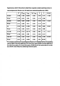
![[PDF] Download Hierarchical Linear Models - Google Sites](https://m.moam.info/img/260x300/pdf-download-hierarchical-linear-models-google-sit_64785cda097c4796708cba0b.jpg)


![[PDF] Read Hierarchical Linear Models: Applications and Data ...](https://m.moam.info/img/260x300/pdf-read-hierarchical-linear-models-applications-a_64789015097c474d228d4a63.jpg)


![[PDF] Hierarchical Linear Models: Applications and Data Analysis ...](https://m.moam.info/img/260x300/pdf-hierarchical-linear-models-applications-and-da_64778da9097c4744708bd6fc.jpg)
![[PDF] Download Hierarchical Linear Models: Applications and Data ...](https://m.moam.info/img/260x300/pdf-download-hierarchical-linear-models-applicatio_6476f8b0097c474c228b5650.jpg)


