ensembles of self-organizing feature maps (SOM). The paper is organized as follows. Background information about single imputation using SOM is presented ...
Multiple imputation of missing data using self organizing map ensembles R. Rallo, J. Ferré and Francesc Giralt# Departament d'Enginyeria Informàtica i Matemàtiques. Escola Tècnica Superior d'Enginyeria. #
Departament d'Enginyeria Química. Escola Tècnica Superior d'Enginyeria Química (ETSEQ).
Universitat Rovira i Virgili. Av. dels Països Catalans, 26, 43007 Tarragona, Catalunya, SPAIN 1. Introduction A virtual sensor is a conceptual device whose output or inferred variable can be modeled in terms of other parameters relevant to the same process. The soft sensor should be conceived at the highest cognitive level of abstraction so that a sufficiently accurate characterization of the total system behavior could be attained in terms of errors between validated or measured data and predicted outputs. Artificial neural networks are an adequate choice because, in addition to the above, they can improve performance with time, i.e., are capable of learning real cause-effect relations between sensor's stimulus and its response when historical databases of the whole process are used for training. Real-time readings of several process variables as well as feedback signals of downstream on-line analyzers for the target property are needed for training the virtual sensor. Once trained, this virtual device uses only real time measurements of the selected process variables obtained by process sensors at certain times to infer the value of the target property. The modeling techniques used implement virtual sensor systems in chemical processing plants usually rely heavily in the quality of the data used to develop the model. Nevertheless, the field sensors used to collect all these data are susceptible to damage and failure due to the manufacturing surroundings. If one of these field sensors fails, the data needed by the model are incomplete making the whole inferential system unusable. This is a major drawback of these data-based approaches. According to Scheffer (2002), data can be Missing Completely at Random (MCAR), Missing at Random (MAR), and Missing not at Random (MNAR). In chemical plants a combination of this three mechanisms is usually responsible for sensor faults. When the values of missing data cannot be recovered several preprocessing methods can be applied. These techniques usually focus on “removing” the missing information, either by ignoring patterns with incomplete information (case deletion) or by substituting the missing variables with plausible values (mean, median, regression, etc.). The shortcomings of case-deletion strategies have been well documented
1
elsewhere (Little and Rubin, 1987). The second approach is the most adequate for conducting the single or multiple imputation processes during virtual sensor operation (Rubin, 1987). The main objective of this work is to develop a multiple imputation strategy based in the use of ensembles of self-organizing feature maps (SOM). The paper is organized as follows. Background information about single imputation using SOM is presented in Section 2. The methodology used to obtain multiple imputations using SOM is described in Section 3. Finally the results obtained for two industrial applications are presented and discussed. 2. The Self-Organizing Map as an Imputation System. The Self-Organizing Map (Kohonen, 1990) is a biologically plausible neural system that induces a topology-preserving mapping from certain high-dimensional space of data onto typically two or three dimensional maps. The relative distances between data points are preserved in the space spanned by the SOM. The map units form a two-dimensional lattice where the location of a map unit carries semantic information about the data assigned to it. Due to the usual two-dimensional layout of the SOM, one can conveniently visualize the resulting cluster densities. SOM consists in a set of units placed on the intersection points of a regular grid. Initially, a reference vector of the same dimension as the data to be classified is assigned to each unit. The learning algorithm is based on a winner-takes-all approach where the unit with the reference vector closer (in terms of Euclidian distance) to the current input data, and all its neighboring units are adapted at each learning step. This process is repeated until the classification stabilizes, i.e. no more adaptations are needed. After this process, each map unit represents a class of the data presented during the training process. The use of the SOM as a single data imputation tool has been explored in diverse application areas (Wang, 2002; Fessant et al., 2002; Rallo et al., 2003), ranging from chemical engineering to social sciences. The process of single imputation using the SOM is based on its capacity to deal with incomplete inputs since the presence of such patterns affects the calculation of distances.As missing components are excluded from the individual variable contributions to distance, the distances corresponding to incomplete patterns will be computed using fewer components. This can be interpreted as the error induced by the projection of the input data onto a lower dimensional space. Since the input components are normalized in the range [0,1] this error is upper-bound by the expression n − n − k , being n the dimension of the input space and k the number of missing variables. If the dimension of the input space is higher than the number of missing variables (n>>k) then the error induced in the calculation of the distance is low. It is important to note that after a proper self-organization process, similar patterns will be associated to neighboring units. This 2
implies that if the error induced by missing variables in the distance calculations leads to a miss assignment of the winner node, the new best matching unit (bmu) selected will be in the neighborhood of the correct one. Under these assumptions the SOM can be used as a data imputation system assuming that for plant applications model degradation will not be linearly correlated with the rate of missing data (Samad and Harp, 1982). 3. Multiple Imputation using Self-Organizing feature maps. In recent years, ensemble approaches to classification and regression have attracted a great deal of interest. These methods can be shown both theoretically and empirically to outperform single predictors in a wide range of tasks (Hansen and Salamon, 1990). The SOM-based single imputation model can be extended to multiple imputation schemes. The main idea resides in the concept of “model aggregation”. Aggregation attempts to improve the quality of the imputed values by generating multiple versions of the imputation system φi (x) , and combining their outputs in some prescribed way, usually by averaging:
φ aggregated ( X ) =
1 N
N
∑ φ ( x) i =1
i
(1)
where φ aggregated (x) is the aggregated imputation system and N is the cardinality of the ensemble.
One of the elements required for accurate prediction when using an ensemble is recognized to be “model diversity", i.e., the disagreement between the components in the ensemble. Diversity can be introduced by (i) manipulating the components of the input data (e.g., using feature selection), (ii) by randomizing the training procedure for each member of the ensemble (e.g., combining underfitted with over-fitted models with different learning parameters and network topologies), (iii) by modifying the response with the addition of noise, and (iv) by re-designing the training set. In the present work two of these main approaches have been used. First, diversity has been introduced in each of the single imputation models by changing the size of the maps. This leads to an ensemble where under-trained models (ie. with great generalization capabilities) coexist with others that have been over-fitted (ie. very accurate and adapted to certain regions of the training data). Second, the training set has been manipulated using “bagging” techniques (Breiman, 1996), i.e., resampling techniques called “bootstrapping” to generate multiple versions of the training set. The procedure starts by considering the training set TR formed by N patterns, each labeled with a probability 1/N. A new training set TRbag is created by sampling with replacement N times from the original training set, using these probabilities. Using this procedure some cases in TR may not appear in TRbag while others may appear multiple times. The resampled training set is used to train
3
an imputation model. The process is repeated several times and the results of each individual model are combined. As mentioned before, the model of single imputation using SOM is based in the estimation of the values of missing variables using the prototypes in the corresponding SOM clusters. These prototypes can be selected and combined using diverse approaches. In this work two approaches were used: (i) direct substitution with the corresponding component taken from the prototype vector of the bmu; (ii) substitution by a mean value obtained by averaging the corresponding components in the prototype vector of the bmu and those of a certain number of its neighboring units. The size of the neighborhood was chosen as three since the inclusion of more distant units doesn’t improve the quality of the imputed data. Furthermore, a n-fold cross validation with n=10 was performed while training model to obtain a more accurate representation of the maps. 3. Results and Conclusions.
Two industrial processes are analyzed to evaluate whether the SOM is a suitable system to perform multiple data imputations and to assess its efficiency compared with mean-substitution and single imputation techniques. The first corresponds to a set of real data records obtained from a polyethylene plant. The polymerization of ethylene to produce LDPE is usually carried out in tubular reactors 800-1500 m long and 20-50 mm in diameter at pressures of 600-3000 bar. The quality of the polymer produced is determined essentially by the Melt Index (mi), which is measured by the flow rate of polymer through a die. The on-line measurement of this quantity is difficult and requires close human intervention because the extrusion die often fools and blocks. As a result, in most plants the mi is evaluated off-line with an analytical procedure that takes between 2 to 4 hours to complete in the laboratory, leaving the process without any real-time quality indicator during this period. A successful model for estimating the mi on-line was developed by Rallo et al. (2002). The main drawback of this approach resides in the fact that the failure of a single sensor makes the virtual sensor unusable. A pool of the LDPE process information, formed by the 148 process variables (pressures, flow rates, temperatures of the cooling/heating streams of the reactor, etc.) closely related to the polymerization process and sampled at intervals of 10 minutes was used to develop a SOM-based multiple imputation system. For simplicity, only one grade of LDPE, containing 5548 input patterns, is discussed here. The data used to train the system included all the 148 variables, with both complete and incomplete patterns. Table 1 summarizes the results obtained using the imputation system under different conditions and using diverse imputation models. Three main
4
cases have been analyzed. First, the effect of random failures in a temperature sensor, second the effects of failures in a flow meter, and finally random failures in any of the 148 sensors. Table 1. Comparison of the imputation models in the LDPE plant for two simulated failures. Absolute mean errors and statistical properties of the imputed dataset (mean, median and variance) for three different levels of missingness. Imputation model Temperature
mean
Sensor Failure
SIbmu
SIneigh=3
µ=0.516 median=0.510
MIbaggingbmu
MIbagging neigh=3
var=0.031 unique=240
MIdimbmu
(4.3%) MIdim neigh=3
Flow rate Measurement
Mean
SIbmu
System Failure
SIneigh=3
MIbaggingbmu µ=0.540 median=0.555 var=0.024
MIbagging neigh=3
MIdimbmu
unique=3084 (56%)
MIdim neigh=3
% missing data
AME
µ
median
var
10% 30% 70% 10% 30% 70% 10% 30% 70% 10% 30% 70% 10% 30% 70% 10% 30% 70% 10% 30% 70% 10% 30% 70% 10% 30% 70% 10% 30% 70% 10% 30% 70% 10% 30% 70% 10% 30% 70% 10% 30% 70%
0.136 0.141 0.142 0.101 0.106 0.106 0.108 0.114 0.115 0.080 0.080 0.074 0.080 0.081 0.077 0.055 0.055 0.053 0.057 0.057 0.054 0.117 0.124 0.125 0.109 0.115 0.117 0.114 0.120 0.121 0.096 0.094 0.095 0.097 0.095 0.096 0.078 0.079 0.079 0.079 0.081 0.081
0.515 0.516 0.515 0.512 0.513 0.515 0.511 0.512 0.512 0.522 0.516 0.518 0.520 0.515 0.517 0.519 0.516 0.516 0.518 0.515 0.516 0.540 0.540 0.544 0.542 0.541 0.544 0.541 0.540 0.543 0.545 0.543 0.545 0.545 0.544 0.544 0.539 0.541 0.542 0.541 0.542 0.543
0.516 0.517 0.520 0.512 0.512 0.515 0.514 0.507 0.511 0.509 0.510 0.511 0.514 0.504 0.500 0.509 0.505 0.497 0.537 0.537 0.534 0.536 0.535 0.539 0.562 0.565 0.564 0.557 0.562 0.561 0.564 0.567 0.564 0.564 0.565 0.564
0.005 0.005 0.005 0.003 0.003 0.003 0.017 0.017 0.018 0.017 0.017 0.017 0.019 0.020 0.021 0.018 0.019 0.020 0.001 0.001 0.001 0.000 0.000 0.000 0.005 0.006 0.005 0.005 0.005 0.005 0.007 0.008 0.008 0.007 0.007 0.007
5
800 700
1.0
600
freq
500 400
0.8
300
100 0 0.0
0.2
0.4
0.6
0.8
1.0
800 700 600
freq
500 400
imputed variable
200
0.6
0.4
10 % missing 30 % missing 70 % missing
0.2
300 200 100
0.0 0.0
0 0.0
0.2
0.4
0.6
0.8
1.0
0.2
0.4
0.6
0.8
1.0
measured variable
normalized data value
Figure 1. (Left) Frequency histograms for the original LDPE data corresponding to the temperature
sensor. (upper) and the flow rate (lower). (Right) Measured and imputed variables corresponding to a set of random failures using the best multiple imputation model. Temperature and flowrate have been chosen because of their distinct distribution of data. Temperature data are smoothly distributed and the amount of unique values is low (4.3%) compared with data corresponding to flowrate, were the amount of unique values raises till 56%. This situation is specially challenging for a prototype-based classifier such is the SOM. In all these situations the models compared had been: mean substitution, SI based on the bmu, SI based on a neighborhood of the bmu, MI using bagging and MI using maps of different size. Also, in each case the effect of the amount of missing data has been studied, varying the missing data ratio from 10% to 70% of the available patterns. Inspection of Table 1 leads to several observations: (i) Regardless of the methods used to construct the individual single imputation systems the absolute mean error of the aggregated response of an ensemble of maps is always lower than that of each individual system; (ii) all imputation systems maintain an stable behavior with the increase of missing data, independently of the imputation technique used. The imputation systems based on the SOM are very robust with respect to the amount of missing data. The performance of these systems (measured as the absolute mean error) does not degrade in a significant way when the amount of missing data increases from 10% up to 6
70%. In all situations, the SOM imputation yield an absolute mean error (AME) lower than that obtained with mean-substitution; (iii) all SOM imputation methods tend to overestimate the value of the mean of the imputed data, while those based solely in mean-substitution are more precise but cannot reproduce well the variance of data. For the temperature sensor, the best imputation model presents a maximum relative error in the mean estimation of 0.6% for the dataset with 10% of missing data. On the other hand, for the flow rate meter, the maximum relative error in the mean for the best model is 0.40% which corresponds to the dataset with 70% of missing data. The variance of a dataset is more difficult to reproduce by means of imputation techniques. For the temperature sensor, the model that reproduces best the variance yields a relative error of 32.2%. The situation is worse for the flow rate, with a relative error around 66.6%. This high value can be explained mainly because the data corresponding to flow rate is more diverse (56% of unique values) than the data for the temperature sensor (4.3%). This high amount of unique values cannot be handled conveniently by prototype-based imputation systems such is the SOM; (iv) All current imputation systems exhibit lower errors for the imputation of temperatures. That constitutes a clear indication of the fact that depending on the statistical properties of data being modeled, imputation systems based on the use of prototype-based classifiers will have low performance. Table 2 summarizes the results obtained in the later case, where the misbehaving sensor is chosen randomly. This situation is equivalent to considering all the sensors in the process plant with the same uniform probability distribution of failure. In this situation, the results observed confirm that SOM-based imputation systems outperform mean-substitution techniques. Figure 1 shows that in all the cases the behavior of the imputation system remains stable independently of the amount of missing data since incomplete patterns were also used during training. Best results are also obtained when using the multiple imputation system implemented using maps of different sizes. To corroborate the quality of the imputation process a hypothesis test to compare the means of the imputed data with the original dataset was also performed. In all the cases, at a significance level of 0.05 this test revealed that there are no statistically significant differences between the means of both samples. Unfortunately significant differences are observed for the variances. The main conclusions that can be drawn from this analysis are: (i) Multiple imputation methods are more stable and outperform those based on single imputation; (ii) the use of an ensemble of SOM maps of different sizes in multiple imputation systems yields better results that techniques based on bagging; (iii) the results obtained using only the components of the prototype of the bmu in SOMbased imputation are better than those obtained using the average with neighboring units.
7
Table 2. Comparison of all the imputation models for a random sensor failure in the LDPE plant. Absolute mean errors for three different levels of missingness Imputation Model Mean
SIbmu
Random sensor Failure
SIneigh=3
MIbaggingbmu
MIbagging neigh=3
MIdimbmu
MIdim neigh=3
% missing data
AME
10% 30% 70% 10% 30% 70% 10% 30% 70% 10% 30% 70% 10% 30% 70% 10% 30% 70% 10% 30% 70%
0.116 0.119 0.119 0.099 0.101 0.100 0.103 0.105 0.105 0.081 0.077 0.073 0.082 0.078 0.075 0.068 0.067 0.065 0.069 0.068 0.066
The second case studied is taken from the UCI Machine Learning Repository (Blake and Merz, 1998). This dataset contains records corresponding to the operation of a Waste Water Treatment Plant (WWTP) under several operating conditions. A schema of the plant with measurement points and variables is provided in Figure 2. One of the most difficult problems in modeling and control these treatment plants is the construction of reliable process models, i.e., the development of detailed first principle models is very difficult, expensive, and time consuming. Activated sludge is a common example of an industrial wastewater treatment process. In this process the inlet flow rate and composition are variable, the population of microorganisms (acting as living catalyst) varies over time (both in quantity and number of species), process knowledge is very limited, and the few available on-line analyzers tend to be unreliable. The amount of organic matter present is measured as biological oxygen demand (BOD), which is a key indicator of water quality. An accurate inferential model for the prediction of BOD is crucial because there is a five-day time delay in laboratory measurements and the aeration tank also has a significant hydraulic time delay. Consequently, the experimental BOD data are not useful for purposes of process control. This benchmark contains 1480 missing values, corresponding to the 7.3% of the whole dataset.
8
Q-E ZN-E PH-E DBO-E DQO-E SS-E SSV-E SED-E COND-E
PH-P DBO-P SS-P SSV-P SED-P COND-P
PH-D DBO-D DQO-D SS-D SSV-D SED-D COND-D
PH-S DBO-S DQO-S SS-S SSV-S SED-S COND-S
Areation Tanks Pretreatment INPUT
Primary Settlers
Secondary Settlers
Primary Treatment Measure Points
RD-DBO-P RD-SS-P RD-SED-P
OUTPUT
Secondary Treatment RD-DBO-S RD-DQO-S
Overall efficiency: RD-DBO-G, RD-DQO-G, RD-SS-G, RD-SED-G
Figure 2. Layout of the WWTP with points of measurement and measured variables.
The whole dataset contains 521 data records, each consisting of 38 process variables. Of these, 29 correspond to measurements taken at different points in the plant (indicated in Figure 1), and the remaining 9 variables correspond to calculated performance measures. The main problem in this dataset resides in the large amount of missing data that contains, making it unusable for training a conventional soft sensor system. Taken into consideration the results fro LDPE, the single imputation methods used to construct the base models for this dataset were based only in the response of the bmu. The full dataset was reconstructed using each of the basic the imputation methods shown in the preceding case. Using these data (without missing information) three virtual sensors for pH, chemical oxygen demand (COD) and biological oxygen demand (BOD) for the effluent water were implemented and trained. All three virtual sensors were based in a neural network trained using the backpropagation algorithm. The whole dataset (512 patterns) was splited into a training set (500 patterns) and the remaining were used for testing purposes. These input patterns were formed only by 22 variables corresponding to measurement points located in the pretreatment, primary settler and secondary settler. The best topology of the neural network was 22-13-1 (ie. 22 input variables, 13 hidden nodes and 1 output). The results obtained in this process are presented in Table 3. It can be seen that the predictions obtained from all the three virtual sensors have a similar value for their absolute mean error. This could be due to the fact that the prediction model is not too sensitive to the quality of the imputations. Nevertheless, it is important to note that the prediction process is possible due to the prior imputation of data. The lowest errors are obtained for BOD, which is the target variable with most missing data in the original dataset (28). A new aggregation model (referred as MIhybrid in the table) for the multiple imputation system was used with this dataset. This model is based in the
9
combination of multiple imputation models based in bagging with those based in maps of different sizes. This improved performance in terms of absolute mean errors. Table 3. Absolute Mean Error for the prediction of pH, COD and BOD at the effluent of the WWTP. Comparison of imputation models. The number of missing cases in the original dataset is shown for each target. Imputation Model AME Mean 0.029 SIbmu 0.032 pH MIbaggingbmu 0.031 Missing: 1 MIdimbmu 0.036 MIhybridbmu 0.026 Mean 0.075 SIbmu 0.065 COD MIbaggingbmu 0.064 Missing: 18 MIdimbmu 0.060 MIhybridbmu 0.058 Mean 0.017 SIbmu 0.021 BOD 0.015 MIbaggingbmu Missing: 23 dim 0.016 MI bmu MIhybridbmu 0.015
References
BLAKE, C.L.., MERZ, C.J., 1998. UCI Repository of machine learning databases, Irvine, University of California, Department of Information and Computer Science. Available from: [http://www.ics.uci.edu/~mlearn/MLRepository.html]. BREIMAN, L., 1996. Bagging Predictors. Machine Learning, 24, 123-140. FESSANT, F., MIDENET, S., 2002. Self-Organising Map for Data Imputation and Correction in Surveys. Neural Comput. & Applic., 10, 300-310. HANSEN, L.K., SALAMON, P. 1990. Neural network ensembles, IEEE Trans. Pattern Analysis and Machine Intelligence, 12(10): 993-1001. KOHONEN, 1990. The Self-Organizing Map. Proc. IEEE. 78, 1443-1464. LITTLE, R.J.A., RUBIN, D.B, 1987. Statistical Analysis with Missing Data. New York: J. Wiley & Sons. RALLO, R., FERRÉ-GINÉ, J., GIRALT, F., 2003. Best Feature Selection and Data Completion for the Design of Soft Neural Sensors. Proceedings of AIChE 2003, 2nd Topical Conference on Sensors, San Francisco. RALLO,.R., FERRÉ-GINÉ, J., ARENAS, A., GIRALT, F., 2002. Neural Virtual Sensor for the Inferential Prediction of Product Quality from Process Variables. Computers and Chemical Engineering, 26 (12), 1735-54. RUBIN, D.B., 1987. Multiple Imputation for Non response in Surveys. New York: J. Wiley & Sons. SAMAD T, HARP S., 1992. Self organisation with partial data. Network, 3, 205–212. SCHEFFER, J., 2002. Dealing with Missing Data. Res. Lett. Inf. Math. Sci., 3, 153. WANG, S., 2003. Application of Self-organising maps for data mining with incomplete data sets. Neural Comput. and Applic., 12, 42-48.
10