Multiple Imputation Using SAS Software - Journal of Statistical Software

JSS

Journal of Statistical Software December 2011, Volume 45, Issue 6.

http://www.jstatsoft.org/

Multiple Imputation Using SAS Software Yang Yuan SAS Institute Inc.

Abstract Multiple imputation provides a useful strategy for dealing with data sets that have missing values. Instead of filling in a single value for each missing value, a multiple imputation procedure replaces each missing value with a set of plausible values that represent the uncertainty about the right value to impute. These multiply imputed data sets are then analyzed by using standard procedures for complete data and combining the results from these analyses. No matter which complete-data analysis is used, the process of combining results of parameter estimates and their associated standard errors from different imputed data sets is essentially the same. This process results in valid statistical inferences that properly reflect the uncertainty due to missing values. This paper reviews methods for analyzing missing data and applications of multiple imputation techniques. This paper presents the SAS/STAT MI and MIANALYZE procedures, which perform inference by multiple imputation under numerous settings. PROC MI implements popular methods for creating imputations under monotone and nonmonotone (arbitrary) patterns of missing data, and PROC MIANALYZE analyzes results from multiply imputed data sets.

Keywords: multiple imputation, monotone missing pattern, Markov chain Monte Carlo.

1. Introduction Most SAS statistical procedures exclude observations with any missing variable values from the analysis. Although using only complete cases is simple, information that is in the incomplete cases is lost. Excluding observations with missing values also ignores the possible systematic difference between the complete cases and incomplete cases, and the resulting inference might not be applicable to the population of all cases, especially with a smaller number of complete cases. There are several approaches to handling missing data. The first approach uses all available data, which ignores any incomplete data in the cases. For example, the CORR procedure estimates a variable mean by using all cases with nonmissing values for this variable, ignoring

2

Multiple Imputation Using SAS Software

the possible missing values in other variables. The CORR procedure also estimates a correlation by using all cases with nonmissing values for this pair of variables. This estimation might make better use of the available data, but the resulting correlation matrix might not be positive definite. Another approach is single imputation, in which a value is substituted for each missing value. Standard statistical procedures for complete data analysis can then be used with the filled-in data set. For example, each missing value can be imputed from the variable mean of the complete cases. This approach treats missing values as if they were known in the completedata analyses. Single imputation does not reflect the uncertainty about the predictions of the unknown missing values, and the resulting estimated variances of the parameter estimates are biased toward zero. Instead of filling in a single value for each missing value, a multiple imputation procedure replaces each missing value with a set of plausible values that represent the uncertainty about the right value to impute (Rubin 1987). The multiply imputed data sets are then analyzed by using standard procedures for complete data and combining the results from these analyses. No matter which complete-data analysis is used, the process of combining results from different data sets is essentially the same. Multiple imputation does not attempt to estimate each missing value through simulated values, but rather to represent a random sample of the missing values. This process results in valid statistical inferences that properly reflect the uncertainty due to missing values; for example, valid confidence intervals for parameters. Multiple imputation inference involves three distinct phases: ˆ The missing data are filled in m times to generate m complete data sets. ˆ The m complete data sets are analyzed by using standard procedures. ˆ The results from the m complete data sets are combined for the inference.

The MI procedure in SAS/STAT software is a multiple imputation procedure that creates multiply imputed data sets for incomplete p-dimensional multivariate data. It uses methods that incorporate appropriate variability across the m imputations. After the m complete data sets are analyzed by using standard procedures, the MIANALYZE procedure can then be used to generate valid statistical inferences about these parameters by combining results from the m complete data sets. Documentation for SAS/STAT 9.2, SAS/STAT 9.22, and SAS/STAT 9.3 is available online (SAS Institute Inc. 2011a).

2. Multiple imputation methods in the MI procedure This section describes methods that are available in PROC MI. PROC MI assumes that the missing data are missing at random (MAR)—that is, the probability that an observation is missing might depend on Yobs , but not on Ymis (Rubin 1976, 1987). Furthermore, PROC MI also assumes that the parameters θ of the data model and the parameters φ of the missing data indicators are distinct. That is, knowing the values of θ does not provide any additional information about φ, and vice versa. If both MAR and distinctness assumptions are satisfied, the missing-data mechanism is said to be ignorable.

Journal of Statistical Software Pattern of missingness Monotone

Type of imputed variable Continuous

Available methods Monotone regression Monotone predicted mean matching Monotone propensity score

Monotone Monotone

Classification (ordinal) Classification (nominal)

Monotone logistic regression Monotone discriminant function

Arbitrary

Continuous

MCMC full-data imputation MCMC monotone-data imputation

3

Table 1: Imputation methods in PROC MI. The imputation method of choice depends on the pattern of missingness in the data and the type of the imputed variable. A data set with variables Y1 , Y2 , . . . , Yp (in that order) is said to have a monotone missing pattern when the event that a variable Yj is missing for a particular individual implies that all subsequent variables Yk , k > j, are missing for that individual. Table 1 summarizes the available methods. For data sets with monotone missing patterns, the variables with missing values can be imputed sequentially with covariates constructed from their corresponding sets of preceding variables. To impute missing values for a continuous variable, one of the following methods can be used: a regression method (Rubin 1987), a predictive mean matching method (Heitjan and Little 1991; Schenker and Taylor 1996), or a propensity score method (Lavori, Dawson, and Shera 1995). To impute missing values for a classification variable, one of the following methods can be used: a logistic regression method when the classification variable has a binary or ordinal response, or a discriminant function method when the classification variable has a binary or nominal response. For data sets with arbitrary missing patterns, a Markov chain Monte Carlo (MCMC) method that assumes multivariate normality can be used to impute missing values (Schafer 1997). The MCMC method can be used to impute either all the missing values or just enough missing values to make the imputed data sets have monotone missing patterns. A monotone missing data pattern offers greater flexibility in the choice of imputation models (such as the monotone regression method) that do not use Markov chains. A different set of covariates can also be specified for each imputed variable. For data sets with arbitrary missing patterns, a fully conditional specification (FCS) method can also be used to impute missing values for both continuous and classification variables (Brand 1999; van Buuren 2007). The FCS method assumes the existence of a joint distribution for all variables. The method does not start with an explicitly specified multivariate distribution for all variables, but rather uses a separate conditional distribution for each imputed variable. This feature is not described further in this paper, but is described in the documentation of the MI procedure for SAS/STAT 9.3 (SAS Institute Inc. 2011b).

2.1. Methods for data sets with monotone missing data patterns For a data set with a monotone missing data pattern, one of the following methods can be used: a regression method, a predictive mean matching method, or a propensity score

4

Multiple Imputation Using SAS Software

method to impute missing values for a continuous variable; a logistic regression method for a classification variable with a binary or ordinal response; or a discriminant function method for a classification variable with a binary or nominal response. For a variable with missing values, a model is fitted using observations with observed values for the variable. With this resulting model, a new model is drawn and is used to impute missing values for the variable. The missing values are imputed sequentially for variables in the order given by the VAR statement. That is, for a variable Yj with missing values, the missing values are imputed from the distribution Yj ∼ P ( Yj | Y1 , Y2 , . . . , Yj−1 ) An example is a regression model Yj = β0 + β1 X1 + β2 X2 + . . . + βk Xk where X1 , X2 , . . ., Xk are the covariates generated from preceding variables Y1 , Y2 , . . . , Yj−1 . The following steps are used to impute missing values for Yj at each imputation: 1. The regression model is fitted using observed values for the variable Yj and its covariates X1 , X2 , ..., Xk . The fitted model includes the regression parameter estimates βˆ = (βˆ0 , βˆ1 , ..., βˆk ) and the associated covariance matrix σ ˆj2 Vj , where Vj is the usual X0 X inverse matrix derived from the intercept and covariates X1 , X2 , ..., Xk . 2 are drawn from the posterior predic2. New parameters β∗ = (β∗0 , β∗1 , ..., β∗(k) ) and σ∗j tive distribution of the parameters (Rubin 1987). That is, they are simulated from (βˆ0 , βˆ1 , ..., βˆk ), σ ˆj2 , and Vj . The variance is drawn as 2 σ∗j =σ ˆj2 (nj − k − 1)/g

where g is a χ2nj −k−1 random variate and nj is the number of nonmissing observations for Yj . The regression coefficients are drawn as 0 β∗ = βˆ + σ∗j Vhj Z 0 is the upper triangular matrix in the Cholesky decomposition, V = V0 V , where Vhj j hj hj and Z is a vector of k + 1 independent random normal variates.

3. The missing values are then replaced by β∗0 + β∗1 x1 + β∗2 x2 + . . . + β∗(k) xk + zi σ∗j where x1 , x2 , ..., xk are the values of the covariates and zi is a simulated normal deviate. The predictive mean matching method can also be used for imputation. It is similar to the regression method except that for each missing value, it imputes an observed value that is selected from the specified number of nearest observations to the predicted value from the simulated regression model (Rubin 1987). The predictive mean matching method ensures that imputed values are plausible, and it might be more appropriate than the regression method if the normality assumption is violated (Horton and Lipsitz 2001).

Journal of Statistical Software

5

2.2. MCMC methods for data sets with arbitrary missing patterns MCMC originated in physics as a tool for exploring equilibrium distributions of interacting molecules. In statistical applications, it is used to generate pseudorandom draws from multidimensional and otherwise intractable probability distributions via Markov chains. A Markov chain is a sequence of random variables in which the distribution of each element depends on the value of the previous one. In MCMC, a Markov chain long enough for the distribution of the elements to stabilize to a common distribution is constructed. This stationary distribution is the distribution of interest. Repeatedly simulating steps of the chain simulates draws from the distribution of interest Schafer (1997). In Bayesian inference, information about unknown parameters is expressed in the form of a posterior probability distribution. MCMC has been applied as a method for exploring posterior distributions in Bayesian inference. That is, through MCMC, the entire joint posterior distribution of the unknown quantities can be simulated and simulation-based estimates of posterior parameters can be obtained. Assuming that the data are from a multivariate normal distribution, data augmentation is applied to Bayesian inference with missing data by repeating the following steps: 1. The imputation I-step: With the estimated mean vector and covariance matrix, the I-step simulates the missing values for each observation independently. That is, if the variables with missing values for observation i are denoted by Yi(mis) and the variables with observed values are denoted by Yi(obs) , then the I-step draws values for Yi(mis) from a conditional distribution Yi(mis) given Yi(obs) . 2. The posterior P-step: The P-step simulates the posterior population mean vector and covariance matrix from the complete sample estimates. These new estimates are then used in the I-step. Without prior information about the parameters, a noninformative prior is used. Other informative priors can also be used. For example, a prior information about the covariance matrix might help stabilize the inference about the mean vector for a near singular covariance matrix. (t+1)

That is, with a current parameter estimate θ(t) at t-th iteration, the I-step draws Ymis from (t+1) p(Ymis |Yobs , θ(t) ) and the P-step draws θ(t+1) from p(θ|Yobs , Ymis ). The two steps are iterated long enough for the results to reliably simulate an approximately independent draw of the missing values for a multiply imputed data set (Schafer 1997).

3. The MI procedure PROC MI provides various methods to create multiply imputed data sets for incomplete multivariate data that can be analyzed using standard SAS procedures. Table 2 summarizes the available statements in PROC MI. The imputation method of choice depends on the pattern of missingness in the data and the type of the imputed variable. For a data set with a monotone missing pattern, the MONOTONE statement can be used to specify applicable monotone imputation methods; otherwise, the MCMC statement can be used assuming multivariate normality.

6

Multiple Imputation Using SAS Software Statement BY CLASS EM

FREQ MCMC MONOTONE TRANSFORM VAR

Description Specifies groups in which separate sets of multiple imputations are performed Specifies the classification variables in the VAR statement Computes the maximum likelihood estimate (MLE) of data with missing values by expectation-maximization (EM) algorithm assuming a multivariate normal distribution Specifies the variable that represents the frequency of occurrence in the observation Specifies Markov chain Monte Carlo imputation methods Specifies imputation methods for a data set with a monotone missing pattern Specifies the variables to be transformed in the imputation process Specifies the variables to be analyzed Table 2: Statements in PROC MI.

Option DATA= NIMPUTE= OUT= ROUND= MINIMUM= MAXIMUM= SEED= MU0=

Description Specifies the input data set Specifies the number of imputations Specifies the output SAS data set in which to put the imputation results Specifies units to round imputed variable values Specifies minimum values for imputed variable values Specifies maximum values for imputed variable values Specifies a positive integer that is used to start the pseudorandom number generator Specifies variable means under the null hypothesis in the t-test for location Table 3: Key options in PROC MI.

The TRANSFORM statement specifies the variables to be transformed before the imputation process; the imputed values of these transformed variables are reverse-transformed to the original forms before the imputation. The Box-Cox, exponential, logarithmic, logit, and power transformations can be used for the variables. Table 3 lists key options available in the PROC MI statement. Often, as few as three to five imputations are adequate in multiple imputation (Rubin 1996). If the NIMPUTE= option is not specified, NIMPUTE=5 is used. The OUT= option specifies the output SAS data set that includes an identification variable, _IMPUTATION_, to identify the imputation number.

3.1. MONOTONE statement The MONOTONE statement specifies monotone methods to impute variables for a data set with a monotone missing pattern. A VAR statement must be specified, and the data set must have a monotone missing pattern with variables ordered in the VAR list. Table 4 lists available methods in the MONOTONE statement. For each imputed variable, the imputation method and, optionally, a set of the effects as covariates to impute the variable can be specified. Each effect is a variable or a combination of variables preceding the imputed variable in the VAR statement. If no covariates are specified, then all preceding variables are used as the covariates.

Journal of Statistical Software Option REG REGPMM PROPENSITY DISCRIM LOGISTIC

Description Specifies the Specifies the Specifies the Specifies the Specifies the

7

regression method predictive mean matching method propensity scores method discriminant function method logistic regression method

Table 4: Summary of imputation methods in MONOTONE statement. With a MONOTONE statement, the variables are imputed sequentially in the order given by the VAR statement. For a continuous variable, the following methods can be used: a regression method, a regression predicted mean matching method, or a propensity score method to impute missing values. For a nominal classification variable, a discriminant function method can be used to impute missing values without using the ordering of the class levels. For an ordinal classification variable, a logistic regression method can be used to impute missing values by using the ordering of the class levels. For a binary classification variable, either a discriminant function method or a logistic regression method can be used.

3.2. Example 1: Regression method for monotone missing pattern data This example uses the regression method to impute missing values for variables in the following Fish data set, which has a monotone missing pattern. The data set contains two species of the fish (Bream and Pike) and three measurements: Length, Height, Width. Some values have been set to missing, and the resulting data set has a monotone missing pattern in the variables Length, Height, Width, and Species. data Fish; title 'Fish Measurement Data'; input Species $ Length Height Width @@; datalines; Bream Bream . Bream Bream . Bream Bream Bream . Bream Bream . Bream Bream Bream

30.0 31.1 34.0 34.5 35.1 36.2 36.4 37.2 38.3 38.6 39.5 39.7 40.5 40.6 41.6 44.1

11.520 12.378 12.444 14.180 14.005 14.263 13.759 14.954 14.860 15.633 15.129 15.523 . 16.362 16.890 18.037

4.020 4.696 . 5.279 4.844 . 4.368 5.171 5.285 5.134 5.570 5.280 . 6.090 6.198 6.306

. Bream Bream Bream Bream Bream Bream Bream Bream Bream . Bream Bream Bream Bream Bream

31.2 33.5 34.7 35.0 36.2 36.2 37.3 37.2 38.5 38.7 39.2 40.6 40.9 41.5 42.6 44.0

12.480 12.730 13.602 12.670 14.227 14.371 13.913 15.438 14.938 14.474 15.994 15.469 16.360 16.517 18.957 18.084

4.306 4.456 4.927 4.690 4.959 4.815 5.073 5.580 5.198 5.728 . 6.131 6.053 5.852 6.603 6.292

8

Multiple Imputation Using SAS Software

Bream Bream Pike Pike Pike . Pike Pike Pike Pike Pike ;

45.3 46.5 34.8 38.8 40.5 45.5 45.8 48.7 55.1 64.0 68.0

18.754 17.624 5.568 5.936 7.290 7.280 7.786 7.792 8.926 9.600 10.812

6.750 6.371 3.376 4.384 4.577 4.323 5.130 4.870 6.171 6.144 7.480

Bream

45.9

18.635

6.747

Pike . Pike Pike Pike Pike . Pike

37.8 39.8 41.0 45.5 48.0 51.2 59.7 64.0

5.708 . 6.396 6.825 6.960 7.680 10.686 9.600

4.158 . 3.977 4.459 4.896 5.376 . 6.144

The following statements invoke the MI procedure and request the regression method for variables Height and Width and the logistic regression method for the variable Species. The resulting data set is named OutFish. proc mi data=Fish seed=1305417 out=OutFish; class Species; monotone reg(Height Width/ details) logistic( Species= Length Height Width Height*Width/ details); var Length Height Width Species; run; The Model Information table describes the method and options used in the multiple imputation process. By default, NIMPUTE=5: five imputations are created for the missing data. The Monotone Model Specification table displays specific monotone methods used in the imputation. The MI Procedure Model Information Data Set Method Number of Imputations Seed for random number generator

WORK.FISH Monotone 5 1305417

Monotone Model Specification

Method

Imputed Variables

Regression Logistic Regression

Height Width Species

The Missing Data Patterns table lists distinct missing data patterns with their corresponding frequencies and percentages. An ‘X’ indicates that the variable is observed in the cor-

Journal of Statistical Software

9

responding group, and a ‘.’ indicates that the variable is missing. The variable means for continuous variables in each group are also displayed. Missing Data Patterns Group 1 2 3 4

Length

Height

Width

Species

X X X X

X X X .

X X . .

X . . .

Freq

Percent

43 3 4 2

82.69 5.77 7.69 3.85

-----------------Group Means---------------Length Height Width

Group 1 2 3 4

41.997674 38.433333 42.275000 40.150000

12.819512 11.797667 13.346750 .

5.359860 4.587667 . .

The DETAILS option in the REG option displays the regression coefficients in the regression model that are estimated from the observed data and the regression coefficients that are used in each imputation. Regression Models for Monotone Method Imputed Variable

Effect

Obs-Data

Height Height

Intercept Length

0.00173 -0.22453

Imputed Variable

Effect

Height Height

Intercept Length

----------------Imputation---------------1 2 3 -0.152270 -0.133455

-0.136544 -0.155687

-0.064801 -0.319043

---------Imputation--------4 5 0.036585 -0.108935

0.088415 -0.215399

Regression Models for Monotone Method Imputed Variable

Effect

Width

Intercept

Obs-Data 0.00682

----------------Imputation---------------1 2 3 0.054140

0.018049

-0.015137

10

Multiple Imputation Using SAS Software

Width Width

Length Height

0.75519 0.73890

Imputed Variable

Effect

Width Width Width

Intercept Length Height

0.838485 0.832117

0.768945 0.831748

0.789577 0.809482

---------Imputation--------4 5 0.024027 0.728779 0.747734

0.084643 0.631217 0.745232

Similarly, the DETAILS option in the LOGISTIC option displays the regression coefficients in the logistic regression model that are estimated from the observed data and the regression coefficients that are used in each imputation. Logistic Models for Monotone Method Imputed Variable

Effect

Species Species Species Species Species

Intercept Length Height Width Height*Width

Obs-Data 22.80713 -14.44698 43.11236 -9.64352 -9.73015

Imputed Variable

Effect

Species Species Species Species Species

Intercept Length Height Width Height*Width

---------------Imputation--------------1 2 3 22.807129 -14.446980 43.112363 -9.643524 -9.730154

22.807129 -14.446980 43.112363 -9.643524 -9.730154

22.807129 -14.446980 43.112363 -9.643524 -9.730154

---------Imputation--------4 5 22.807129 -14.446980 43.112363 -9.643524 -9.730154

22.807129 -14.446980 43.112363 -9.643524 -9.730154

The following statements list the first 10 observations of OutFish with imputed values. proc print data=OutFish(obs=10); var _Imputation_ Species Length Height Width; title 'First 10 Observations of the Imputed Data Set'; run; First 10 Observations of the Imputed Data Set Obs

_Imputation_

Species

Length

Height

Width

Journal of Statistical Software 1 2 3 4 5 6 7 8 9 10

1 1 1 1 1 1 1 1 1 1

Bream Bream Bream Bream Bream Bream Bream Bream Bream Bream

30.0 31.2 31.1 33.5 34.0 34.7 34.5 35.0 35.1 36.2

11 11.520 12.480 12.378 12.730 12.444 13.602 14.180 12.670 14.005 14.227

4.02000 4.30600 4.69600 4.45600 4.62964 4.92700 5.27900 4.69000 4.84400 4.95900

3.3. MCMC statement The MCMC statement uses a Markov chain Monte Carlo method to impute values for a data set with an arbitrary missing pattern, assuming a multivariate normal distribution for the data. Table 5 summarizes the key options available for the MCMC statement. The key options for the imputation details are: ˆ CHAIN=SINGLE | MULTIPLE: The CHAIN= option specifies whether a single chain (CHAIN=SINGLE) is used for all imputations or a separate chain (CHAIN=MULTIPLE) is used for each imputation (Schafer 1997). The default is CHAIN=SINGLE. ˆ IMPUTE=MONOTONE | FULL: The IMPUTE= option specifies whether a full-data imputation (IMPUTE=FULL) is used for all missing values or a monotone-data imputation (IMPUTE=MONOTONE) is used for a subset of missing values to make the imputed data sets have a monotone missing pattern. The default is IMPUTE=FULL.

Option Data sets INEST= OUTEST= OUTITER=

Description Inputs parameter estimates for imputations Outputs parameter estimates used in imputations Outputs parameter estimates used in iterations

Imputation details CHAIN= IMPUTE= NBITER= NITER=

ODS output graphics PLOTS=TRACE PLOTS=ACF

Specifies single or multiple chain Specifies monotone or full imputation Specifies the number of burn-in iterations for each chain Specifies the number of iterations between imputations in a chain

Displays trace plots of parameters from iterations Displays autocorrelation plots of parameters from iterations

Table 5: Summary of key options in MCMC statement.

12

Multiple Imputation Using SAS Software ˆ NBITER=numbers: The NBITER= option specifies the number of burn-in iterations before the first imputation in each chain. The default is NBITER=200. ˆ NITER=numbers The NITER= option specifies the number of iterations between imputations in a single chain. The default is NITER=100.

3.4. Example 2: MCMC method for arbitrary missing pattern data This example uses the MCMC method to impute missing values for variables in a data set with an arbitrary missing pattern. The following Fitness data set has been altered to contain an arbitrary missing pattern. These measurements were made on men involved in a physical fitness course at N.C. State University. Certain values have been set to missing and the resulting data set has an arbitrary missing pattern. Only selected variables of Oxygen (intake rate, ml per kg body weight per minute), Runtime (time to run 1.5 miles in minutes), RunPulse (heart rate while running) are used. data Fitness; input Oxygen datalines; 44.609 11.37 54.297 8.65 49.874 9.22 . 11.95 39.442 13.08 50.541 . 44.754 11.12 51.855 10.33 40.836 10.95 46.774 10.25 39.407 12.63 45.441 9.63 45.118 11.08 45.790 10.47 48.673 9.40 47.467 10.50 ;

RunTime RunPulse @@; 178 156 . 176 174 . 176 166 168 . 174 164 . 186 186 170

45.313 59.571 44.811 . 60.055 37.388 47.273 49.156 46.672 50.388 46.080 . 39.203 50.545 47.920

10.07 . 11.63 10.85 8.63 14.03 . 8.95 10.00 10.08 11.17 8.92 12.88 9.93 11.50

185 . 176 . 170 186 . 180 . 168 156 . 168 148 170

The following statements use the MCMC method to impute missing values for all variables in a data set. The resulting data set is named OutFitness. These statements also create an iteration plot for the successive estimates of the variable Oxygen and an autocorrelation function plot for Oxygen. ods graphics on; proc mi data=Fitness nimpute=4 seed=501213 mu0=50 10 180 out=OutFitness; em; mcmc plots=(trace(mean(Oxygen)) acf(mean(Oxygen)));

Journal of Statistical Software

13

var Oxygen RunTime RunPulse; run; ods graphics off; The Model Information table describes the method and options used. The MI Procedure Model Information Data Set Method Multiple Imputation Chain Initial Estimates for MCMC Start Prior Number of Imputations Number of Burn-in Iterations Number of Iterations Seed for random number generator

WORK.FITNESS MCMC Single Chain EM Posterior Mode Starting Value Jeffreys 4 200 100 501213

By default, the procedure uses a single chain to create five imputations. It takes 200 burn-in iterations before the first imputation and 100 iterations between imputations. The burn-in iterations are used to make the iterations converge to the stationary distribution before the imputation. The Missing Data Patterns table lists distinct missing data patterns. It shows that the data set does not have a monotone missing pattern. Missing Data Patterns

Group 1 2 3 4 5

Group 1 2 3 4 5

Oxygen

Run Time

Run Pulse

X X X . .

X X . X X

X . . X .

Freq

Percent

21 4 3 1 2

67.74 12.90 9.68 3.23 6.45

-----------------Group Means---------------Oxygen RunTime RunPulse 46.353810 47.109500 52.461667 . .

10.809524 10.137500 . 11.950000 9.885000

171.666667 . . 176.000000 .

14

Multiple Imputation Using SAS Software

The expectation-maximization (EM) algorithm is a technique that finds maximum likelihood estimates for parametric models for incomplete data (Little and Rubin 2002). By default, the procedure uses the statistics from the available cases in the data as the initial estimates for EM algorithm, and the correlations are set to zero. With the EM statement, the initial parameter estimates for the EM algorithm and the resulting maximum likelihood estimates are displayed. Initial Parameter Estimates for EM _TYPE_

_NAME_

MEAN COV COV COV

Oxygen RunTime RunPulse

Oxygen

RunTime

RunPulse

47.116179 29.301078 0 0

10.688214 0 1.904067 0

171.863636 0 0 102.885281

EM (MLE) Parameter Estimates _TYPE_

_NAME_

MEAN COV COV COV

Oxygen RunTime RunPulse

Oxygen

RunTime

RunPulse

47.104077 27.797931 -6.457975 -18.031298

10.554858 -6.457975 2.015514 3.516287

171.381669 -18.031298 3.516287 97.766857

The EM algorithm can also be used to compute posterior modes, the parameter estimates with the highest observed-data posterior density. These posterior modes are used to begin the MCMC process. EM (Posterior Mode) Estimates _TYPE_

_NAME_

MEAN COV COV COV

Oxygen RunTime RunPulse

Oxygen

RunTime

RunPulse

47.103766 24.549967 -5.726112 -15.926036

10.554320 -5.726112 1.781407 3.124798

171.382196 -15.926036 3.124798 83.164045

After the completion of the specified four imputations, the Variance Information table displays the between-imputation variance, within-imputation variance, and total variance for combining complete-data inferences. Variance Information

Variable

-----------------Variance----------------Between Within Total

DF

Journal of Statistical Software Oxygen RunTime RunPulse

0.067395 0.000211 0.801827

0.962300 0.064026 3.441013

15 1.046544 0.064290 4.443298

24.54 28.062 15.929

Variable

Relative Increase in Variance

Fraction Missing Information

Relative Efficiency

Oxygen RunTime RunPulse

0.087544 0.004129 0.291276

0.084443 0.004123 0.250570

0.979326 0.998970 0.941050

The Parameter Estimates table displays the estimated mean and standard error of the mean for each variable. The table also displays a 95% confidence interval for the variable mean and a t statistic with the associated p-value for the hypothesis that the population mean is equal to the value specified with the MU0= option. Parameter Estimates Variable

Mean

Std Error

Oxygen RunTime RunPulse

47.129771 10.583493 172.041037

1.023007 0.253555 2.107913

95% Confidence Limits 45.0208 10.0642 167.5708

49.2387 11.1028 176.5112

DF 24.54 28.062 15.929

Variable

Minimum

Maximum

Mu0

t for H0: Mean=Mu0

Pr > |t|

Oxygen RunTime RunPulse

46.783898 10.570896 170.934337

47.395550 10.599616 173.122002

50.000000 10.000000 180.000000

-2.81 2.30 -3.78

0.0097 0.0290 0.0017

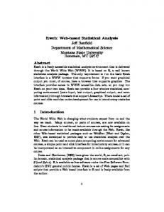
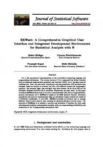
With the TRACE(MEAN(OXYGEN)) option, the procedure displays a trace plot for the mean of Oxygen, as shown in Figure 1. The plot shows no apparent trends for the variable Oxygen. With the ACF(MEAN(OXYGEN)) option, an autocorrelation plot for the mean of Oxygen is displayed, as shown in Figure 2. It shows no significant positive or negative autocorrelation. The following statements list the first 10 observations of the output data set OutFitness: proc print data=OutFitness(obs=10); title 'First 10 Observations of the Imputed Data Set'; run; First 10 Observations of the Imputed Data Set Run

16

Multiple Imputation Using SAS Software

Figure 1: Trace plot for Oxygen.

Figure 2: Autocorrelation function plot for Oxygen.

Journal of Statistical Software

17

Obs

_Imputation_

Oxygen

RunTime

Pulse

1 2 3 4 5 6 7 8 9 10

1 1 1 1 1 1 1 1 1 1

44.6090 45.3130 54.2970 59.5710 49.8740 44.8110 42.8857 46.9992 39.4420 60.0550

11.3700 10.0700 8.6500 8.0747 9.2200 11.6300 11.9500 10.8500 13.0800 8.6300

178.000 185.000 156.000 155.925 176.837 176.000 176.000 173.099 174.000 170.000

4. Combining inferences from imputed data sets With m imputations, m different sets of the point and variance estimates for a parameter Q can be computed. Let Qˆi and Uˆi be the point and variance estimates from the ith imputed data set, i=1, 2, ..., m. Then the point estimate for Q from multiple imputations is the average of the m complete-data estimates: Q=

m 1 X Qˆi m i=1

Let U be the within-imputation variance, which is the average of the m complete-data estimates m 1 X Uˆi U= m i=1

and B be the between-imputation variance B=

m 1 X (Qˆi − Q)2 m − 1 i=1

Then the variance estimate associated with Q is the total variance T = U + (1 +

1 )B m

The statistic (Q − Q)T −1/2 is approximately distributed as a t distribution with vm degrees of freedom (Rubin 1987), where "

vm

U = (m − 1) 1 + (1 + m−1 )B

#2

When the complete-data degrees of freedom v0 is small and there is only a modest proportion of missing data, the computed degrees of freedom, vm , can be much larger than v0 , which

18

Multiple Imputation Using SAS Software Statement BY CLASS MODELEFFECTS STDERR TEST

Description Specifies groups in which separate sets of multiple imputations are performed Specifies classification variables in the MODELEFFECTS statement Lists the effects in the data set to be analyzed Lists standard errors associated with effects Tests linear hypotheses about the parameters Table 6: Statements in PROC MIANALYZE.

is inappropriate. Barnard and Rubin (1999) recommend the use of an adjusted degrees of ∗ , freedom, vm ∗ vm



=

where vobs ˆ =

1 1 + vm vobs ˆ

−1

v0 + 1 v0 (1 − γ) v0 + 3

γ=

(1 + m−1 )B T

5. The MIANALYZE procedure From m imputations, m different sets of the point and variance estimates for a parameter Q can be computed. PROC MIANALYZE combines these results and generates valid statistical inferences about the parameter. Multivariate inferences can also be derived from the m imputed data sets. Table 6 lists available statements in PROC MIANALYZE. The MODELEFFECTS statement lists the effects in the data set to be analyzed. Each effect is a variable or a combination of variables, and is specified with a special notation using variable names and operators. The STDERR statement lists standard errors associated with effects in the MODELEFFECTS statement, when the input DATA= data set contains both parameter estimates and standard errors as variables in the data set. The TEST statement tests linear hypotheses about the parameters β. An F test is used to test jointly the null hypotheses (H0 : Lβ = c) specified in a single TEST statement. Table 7 lists available options in the PROC MIANALYZE statement. Input data sets are specified based on the requested type of inference. The appropriate combination depends on the type of inference and the SAS procedure that was used to create the data sets. For example, if PROC REG was used to create an OUTEST= data set of type EST that contains the parameter estimates and covariance matrix, the DATA= option would be used to read the OUTEST= data set.

5.1. Example 3: Reading results from PARMS= and COVB= data sets This example creates data sets that contain parameter estimates and corresponding covariance

Journal of Statistical Software Option Input data sets DATA= DATA=

19

Description

PARMS= PARMINFO= COVB= XPXI=

Specifies the input Specifies the input standard errors Specifies the input Specifies the input Specifies the input Specifies the input

COV, CORR, or EST type data set data set for parameter estimates and

Statistical analysis ALPHA= EDF= THETA0=

Specifies the level for the confidence interval Specifies the complete-data degrees of freedom Specifies parameters under the null hypothesis

Printed output WCOV BCOV TCOV MULT

Displays Displays Displays Displays

data data data data

set set set set

for for for for

parameter estimates parameter information covariance matrices (X0 X)−1 matrices

the within-imputation covariance matrix the between-imputation covariance matrix the total covariance matrix multivariate inferences

Table 7: Options in PROC MIANALYZE. matrices computed by a logistic regression model for imputed data sets. These estimates are then combined to generate valid statistical inferences about the model parameters. The following statements use PROC LOGISTIC to generate the parameter estimates and covariance matrix for each imputed data set stored in OutFish: proc logistic data=OutFish; class Species; model Species= Length / covb; by _Imputation_; ods output ParameterEstimates=lgparms CovB=lgcovb; run; The following statements display the ODS output PARAMETERESTIMATES= data set from PROC LOGISTIC for the first two imputed data sets: proc print data=lgparms(obs=4); title 'Logistic Model Coefficients (First Two Imputations)'; var _Imputation_ Variable Estimate StdErr; run; The Logistic Model Coefficients (First Two Imputations) table displays the output parameter estimates and standard errors for the first two imputed data sets. Logistic Model Coefficients (First Two Imputations)

20

Multiple Imputation Using SAS Software Obs 1 2 3 4

_Imputation_

Variable

Estimate

StdErr

1 1 2 2

Intercept Length Intercept Length

11.6446 -0.2599 10.9976 -0.2477

3.5105 0.0836 3.3477 0.0802

The following statements display the ODS output COVB= data set from PROC LOGISTIC for the first two imputed data sets: proc print data=lgcovb(obs=4); title 'Logistic Covariance Matrices (First Two Imputations)'; run; The Logistic Covariance Matrices (First Two Imputations) table displays the output covariance matrices for the first two imputed data sets. Logistic Covariance Matrices (First Two Imputations) Obs 1 2 3 4

_Imputation_

Parameter

Intercept

1 1 2 2

Intercept Length Intercept Length

12.3239 -0.29171 11.20695 -0.26691

Length -0.29171 0.006986 -0.26691 0.006433

The following statements use the MIANALYZE procedure to read parameter estimates in the PARMS= data set and the associated covariance matrix in the COVB= data set: proc mianalyze parms=lgparms covb=lgcovb; modeleffects Intercept Length; run; The Model Information table lists the input data sets and the number of imputations. The Variance Information table displays the between-imputation, within-imputation, and total variances for combining complete-data inferences. The MIANALYZE Procedure Model Information PARMS Data Set COVB Data Set Number of Imputations

WORK.LGPARMS WORK.LGCOVB 5

Variance Information

Journal of Statistical Software

Parameter

21

-----------------Variance----------------Between Within Total

Intercept Length

0.372426 0.000126

12.323246 0.006976

12.770157 0.007127

DF 3266 8927.7

Parameter

Relative Increase in Variance

Fraction Missing Information

Relative Efficiency

Intercept Length

0.036266 0.021625

0.035587 0.021386

0.992933 0.995741

The Parameter Estimates table displays the parameter estimate and standard error of the regression coefficient for each variable. With an estimate −0.25906 and its associated p-value 0.0022 for the parameter Length, the length of Bream is significantly shorter than the length of Pike. Parameter Estimates Parameter

Estimate

Std Error

Intercept Length

11.614996 -0.259060

3.573536 0.084419

95% Confidence Limits 4.60840 -0.42454

18.62159 -0.09358

Parameter

Minimum

Maximum

Intercept Length

10.997552 -0.270055

12.217637 -0.247650

Parameter

Theta0

t for H0: Parameter=Theta0

Pr > |t|

Intercept Length

0 0

3.25 -3.07

0.0012 0.0022

DF 3266 8927.7

5.2. Example 4: Reading results from a DATA= data set This example creates an EST-type data set that contains regression coefficients and their corresponding covariance matrices computed from imputed data sets. These estimates are then combined to generate valid statistical inferences about the regression model. The following statements use the REG procedure to generate regression coefficients in each imputed data set stored in OutFitness:

22

Multiple Imputation Using SAS Software proc reg data=OutFitness outest=regest covout noprint; model Oxygen= RunTime RunPulse; by _Imputation_; run;

The following statements display the output OUTEST= data set from PROC REG for the first two imputed data sets: proc print data=regest(obs=8); var _Imputation_ _Type_ _Name_ Intercept RunTime RunPulse; title 'REG Model Coefficients (First Two Imputations)'; run; The REG Model Coefficients (First Two Imputations) table displays regression coefficients and their covariance matrices for the first two imputed data sets. REG Model Coefficients (First Two Imputations) Obs 1 2 3 4 5 6 7 8

_Imputation_

_TYPE_

1 1 1 1 2 2 2 2

PARMS COV COV COV PARMS COV COV COV

_NAME_

Intercept RunTime RunPulse Intercept RunTime RunPulse

Intercept

RunTime

RunPulse

95.0397 66.8696 -0.8169 -0.3371 92.0495 81.2318 -0.8646 -0.4150

-3.39792 -0.81692 0.14815 -0.00436 -3.29472 -0.86457 0.13230 -0.00308

-0.06817 -0.33708 -0.00436 0.00223 -0.06029 -0.41496 -0.00308 0.00259

The following statements combine the results from the imputed data sets: proc mianalyze data=regest edf=28; modeleffects Intercept RunTime RunPulse; run; The EDF= option is specified to request that the adjusted degrees of freedom be used in the analysis. For a regression model with three independent variables (including the Intercept) and 31 observations, the complete-data error degrees of freedom is 28. The Model Information table lists the input data set and the number of imputations. The Variance Information table displays the between-imputation, within-imputation, and total variances for combining complete-data inferences. The MIANALYZE Procedure Model Information Data Set

WORK.REGEST

Journal of Statistical Software Number of Imputations

23

4

Variance Information

Parameter

-----------------Variance----------------Between Within Total

Intercept RunTime RunPulse

8.872382 0.022390 0.000119

80.351747 0.137756 0.002602

91.442225 0.165744 0.002750

DF 20.683 18.038 24.191

Parameter

Relative Increase in Variance

Fraction Missing Information

Relative Efficiency

Intercept RunTime RunPulse

0.138024 0.203169 0.057212

0.129776 0.184223 0.055958

0.968575 0.955972 0.986204

The Parameter Estimates table displays the parameter estimate and standard error of the regression coefficient for each variable. The table also displays a 95% mean confidence interval and a t test with the associated p-value for the hypothesis that the regression coefficient is equal to zero. Since the p-value for RunPulse is 0.2987, this variable can be removed from the regression model. Parameter Estimates Parameter

Estimate

Std Error

Intercept RunTime RunPulse

91.220141 -3.260213 -0.055700

9.562543 0.407116 0.052445

95% Confidence Limits 71.31514 -4.11540 -0.16390

111.1251 -2.4050 0.0525

Parameter

Minimum

Maximum

Intercept RunTime RunPulse

88.378636 -3.397916 -0.068166

95.039651 -3.047243 -0.042970

Parameter

Theta0

t for H0: Parameter=Theta0

Pr > |t|

DF 20.683 18.038 24.191

24

Multiple Imputation Using SAS Software Intercept RunTime RunPulse

0 0 0

9.54 -8.01 -1.06