Amy J. Briggs. Department of Computer Science. Middlebury College. Middlebury, VT 05753. {dfouhey, schar, briggs}@middlebury.edu. AbstractâWe present a ...
In Proc. 20th International Conference on Pattern Recognition (ICPR 2010), Istanbul, Turkey, August 2010
Multiple Plane Detection in Image Pairs using J-Linkage David F. Fouhey
Daniel Scharstein
Amy J. Briggs
Department of Computer Science Middlebury College Middlebury, VT 05753 {dfouhey, schar, briggs}@middlebury.edu
Abstract—We present a new method for the robust detection and matching of multiple planes in pairs of images. Such planes can serve as stable landmarks for vision-based urban navigation. Our approach starts from SIFT matches and generates multiple local homography hypotheses using the recent J-linkage technique by Toldo and Fusiello, a robust randomized multi-model estimation algorithm. These hypotheses are then globally merged, spatially analyzed, robustly fitted, and checked for stability. When tested on more than 30,000 image pairs taken from panoramic views of a college campus, our method yields no false positives and recovers 72% of the matchable building walls identified by a human, despite significant occlusions and viewpoint changes. Keywords-3D shape recovery; perceptual organization; stereo and motion.
I. I NTRODUCTION AND RELATED WORK Given two images of a scene containing planar surfaces, the points in each pair of corresponding planar regions are related by a homography, a linear projective transformation with 8 parameters. Detecting such homographies—and thus the underlying 3D planes—has many applications, including camera calibration, 3D architectural reconstruction, and robot navigation. In this paper we consider the use of the detected planes for visual navigation [1] and location recognition [2] from a set of panoramic reference views (see Fig. 1). While visual features such as SIFT [3] can be used for localization [4], such features are unstable in the presence of repetitive structures such as windows in building facades and often yield false positives. Instead, we propose using entire planar surfaces as visual features. We thus need a robust way of extracting and matching multiple planes from image pairs, even in the presence of significant viewpoint changes and occlusion. Our approach is to establish multiple homography hypotheses starting from matched SIFT features. There is much existing work on estimating homographies from matched features. The standard approach for model estimation in the presence of outliers is Random Sample Consensus (RANSAC); however, it cannot detect multiple models. Both Vincent and Laganiere [5] and Kanazawa and Kawakami [6] use sequential approaches to overcome this problem. Zuliani et al. [7] compare sequential RANSAC with multiRANSAC. All of these approaches commit to
Figure 1. Corresponding planar surfaces detected by our method between two multi-image panoramas. Each planar surface is modeled by a homography relating a collection of matched SIFT features. The detected planes can serve as stable landmarks for location recognition and visual navigation.
plane hypotheses sequentially or require specifying the number of models a priori. Similar non-randomized methods commit to initial seed regions that are then grown while updating the models [8], [9]. Like several of the above methods, our approach performs randomized model estimation on feature correspondences; in contrast to existing work, however, it does not sequentially commit to hypotheses. Instead we use the J-linkage technique by Toldo and Fusiello [10], a robust randomized multi-model estimation algorithm, followed by a number of steps to ensure high accuracy while avoiding false positives. II. A PPROACH Given an image pair, our method extracts feature correspondences, establishes initial plane hypotheses using Jlinkage, and globally merges them. The resulting hypotheses are then refined using spatial analysis and stability checks. Each step is discussed in detail below. A. Feature correspondence extraction To generate feature correspondences we use the SIFT detector and matching procedure [3]. The feature detector is applied to the two grayscale images, producing collections of features I1 and I2 . Correspondences between these features are established using a nearest-neighbor search in the feature descriptor space. For each feature p ∈ I1 we find its nearest
and second-nearest neighbor q, q 0 ∈ I2 respectively. The correspondence between p and q is accepted if the Euclidean distance ratio |p − q|/|p − q 0 | is below a constant bound. For a correspondence c = (p, q), we denote its feature locations in the two images as xc1 and xc2 respectively. B. Initial hypotheses using J-linkage Randomized model estimation techniques such as RANSAC provide an effective and efficient way to generate models from outlier-contaminated data. In order to detect multiple models we adopt the recent J-linkage technique [10], which is robust to gross outliers and noise and does not require prior specification of the number of models. We use it here to detect perspective transformations (homographies) that map planar surfaces from one image to the other. Like RANSAC, J-linkage starts with k randomly chosen minimum sample sets (MSS). In our case each MSS contains 4 correspondences, which uniquely specify a homography. In order to increase the likelihood of choosing an MSS comprised of inliers, we draw the first correspondence uniformly, and the remaining three with higher probability in the vicinity of the first [10]. Let H1 , . . . , Hk denote the homographies specified by each MSS. For each correspondence c, we then compute its preference set Pc , the subset of models that fit c well enough: Pc = {Hj : errHj (c) < �, 1 ≤ j ≤ k, }, |H(xc1 )
(1)
xc2 |
where errH (c) = − is the reprojection error of correspondence c under transformation H, and � is a constant error threshold (we use � = 1.5 pixels). The preference set of a set of correspondences is defined as the intersection of their individual preference sets. Next, J-linkage performs agglomerative clustering: beginning with singleton sets of the detected correspondences, a pair of sets with minimum Jaccard distance dJ between their preference sets is merged, where dJ (X, Y ) = (|X ∪ Y | − |X ∩ Y |)/|X ∪ Y |.
(2)
Merging proceeds until the minimum distance is 1, i.e., all preference sets are disjoint. At every stage of the method, a set of supporting correspondences represents a plane hypothesis. It is easy to see that each cluster of correspondences must always contain at least one model that fits all of them. Many outliers will remain in small sets, and are discarded at this stage; throughout the method, we require at least 6 supporting correspondences for a valid model. The remaining disjoint sets of sufficient cardinality are treated as the initial plane hypotheses. Fig. 2a illustrates the results of this step. C. Global merging Since most of the initial hypotheses are generated from groups of nearby points, globally visible aspects of the
(a) Plane hypotheses after J-linkage
(b) Plane hypotheses after global merging
(c) Plane hypotheses after spatial analysis Figure 2. Illustration of the individual steps of our method. Feature locations are marked with dots; plane hypotheses are visualized using color and convex hulls. (a) J-linkage output; note that single planes often result in multiple models. (b) Global merging reduces the number of models but does not eliminate “rogue” correspondences that fit a model by chance. (c) Spatial analysis retains only compact feature sets.
perspective transformation, such as foreshortening, may be effectively underdetermined. J-linkage only merges correspondences that share a common model, so a large planar surface in the scene may result in several plane hypotheses that cannot be merged, as can be observed in Fig. 2a. We therefore continue the agglomerative clustering, but use a different distance function dF that measures the average error for the model that best fits the union of correspondences: dF (X, Y ) =
X 1 errHˆ (c), |X ∪ Y |
(3)
c∈X∪Y
ˆ is the least-squares solution to the perspective where H transformation for X ∪ Y . Clustering is stopped when the minimum distance exceeds the threshold � used in the Jlinkage step. Fig. 2b illustrates the results. The reason that the green triangle on the left is not merged with the dominant red hypothesis is that the green hypothesis represents a plane different from the main building wall due
Figure 3. Spatial analysis. The red points initially belong to a single plane hypothesis; they are triangulated and long edges are removed. The resulting disjoint graphs are then split into separate hypotheses; the one on the left is rejected due to an insufficient number of supporting points.
to erroneous matches, which is a common problem with repetitive features such as windows of a building. Thus, the two hypotheses are not matched, and in fact the green hypothesis is later removed due its insufficient number of supporting matches.
points in a model are more or less collinear. In this case, slight perturbations in feature locations would result in large changes in the underlying models. Since our goal is to use the detected planes as stable visual landmarks, we want to eliminate such unstable models. We use a simple perturbation test to detect them. Specifically, we repeatedly disturb the feature locations in both images using normally-distributed noise proportional to the size of their bounding box, compute the best-fit model, and project the corners of the bounding box under this model. For a stable model based on well-distributed features, the standard deviations of the bounding box corners will be of the same magnitude as the perturbation noise; if they are significantly higher, we reject the model. The plane hypotheses that pass this test are the final output of our method. The result of the approach when run on image pairs between two multi-image panoramas is shown in Fig. 1. III. R ESULTS
D. Spatial analysis The plane hypotheses computed at this point accurately capture the planar surfaces present in the 3D scene, but may also contain additional “rogue” correspondences that match the underlying transformations by chance (see for instance the yellow correspondence on the far right in Fig. 2b). This is because analysis so far has considered only the feature descriptor and homography spaces, but not the feature location space. Such outliers with respect to feature locations are problematic if we want to estimate the extent of the plane, for instance using the convex hull of the feature points. We detect and eliminate “rogue” correspondences by computing for each plane hypothesis the Delaunay triangulation of its feature locations in image 1, and removing all edges whose length is more than one standard deviation over the mean (see Fig. 3). We then treat the disconnected subgraphs as separate hypotheses and reject those that are insufficiently supported (i.e., have fewer than 6 correspondences). The remaining hypotheses are passed on to the final step. See Fig. 2c for illustration. E. Robust fitting and stability checks Since the distance function dF used in global merging measures the average (rather than maximum) error, we perform a final robust fitting step for each model C to improve its accuracy and remove remaining outliers. We repeatedly compute the best-fit (least-squares) homography ˆ for C, and remove correspondences c from C for which H errHˆ (c) > �i , using a sequence of decreasing error thresholds {�i }. We start with a large threshold and gradually lower it to the original threshold �. If C becomes insufficiently supported during this process, it is rejected. A different problem is that some of the transformations may be effectively underdetermined, for instance, if all
We tested our method using panoramic sequences taken from 31 different viewpoints on Middlebury’s campus. Each sequence spans 360 degrees and contains 8 or 9 images, for a total of 259 images. Each image is corrected for radial distortion, scaled to a width of 1500 pixels, and converted to grayscale for SIFT processing. We evaluated our planedetection method by running it on all 32,455 inter-viewpoint image pairs. Since the viewpoints are spread out over a fairly wide area, most of these pairs do not contain common planes. We manually analyzed the images in order to enable a quantitative performance evaluation. Overall, we found 330 instances of planes that are commonly visible in pairs of images. In 108 of them, however, the SIFT detector fails to find any features, due to the lack of texture (for instance, on building roofs). Another 87 of the plane pairs we identified are too small or undergo too severe a viewpoint shift for SIFT to establish a sufficient number of correspondences. Since the SIFT features are the input to our method, we cannot expect these planes to be found. The remaining 135 “detectable” planes still contain formidable challenges, including illumination changes, reflections (e.g., windows), significant occlusion (e.g., by trees), and significant viewpoint and scale changes. Our method finds 97 of these planes, about 72%. Impressively, despite a data set containing large numbers of similar planes, not a single plane is erroneously detected, indicating the effectiveness of our spatial analysis and stability checks. Figure 4 illustrates the accuracy of our method on a challenging example: two views of a building facade with a significant viewpoint shift, a scale change of more than 300%, and many unmatchable areas (doorway and windows). Despite these challenges our method accurately detects and aligns the building wall.
the Delaunay triangulation of feature locations. Finally, to ensure the quality of the resulting planes, we perform robust fitting and a stability check. Our experimental results on a large number of images demonstrate the effectiveness of our method in sufficiently textured environments. ACKNOWLEDGMENTS We are grateful to Porter Westling for taking the panorama photos. Support for this work was provided by the National Science Foundation under grant IIS-0713442. R EFERENCES [1] D. Robertson and R. Cipolla, “An image based system for urban navigation,” in Proceedings of the British Machine Vision Conference, 2004. [2] G. Schindler, M. Brown, and R. Szeliski, “City-scale location recognition,” in Proceedings of the IEEE Conference on Computer Vision and Pattern Recognition, 2007. Figure 4. Alignment performance in the presence of significant scale and viewpoint changes. Top row: Cropped regions of a matched image pair. Yellow dots mark features belonging to the model; magenta crosses mark other features. Bottom left: The second image warped by the aligning homography. Bottom right: The difference image visualizing the quality of the alignment (dark regions indicate low differences). Note that the building wall is perfectly aligned.
We also performed experiments assessing the effectiveness and necessity of the individual steps of our method. We used a fixed set of image pairs and ran the method, selectively removing one of the post-initial estimation steps at a time. In all cases, the performance decreased, resulting in planes that were detected in pieces, poorly localized, poorly registered, or missed altogether, Finally, we want to point out that distinct 3D surfaces do not always result in separate detected planes. For instance, in Fig. 2c, the three visible faces of the octagonal tower are detected as a single plane. This is not a flaw of the algorithm but rather a limitation of the problem formulation: if the viewpoint does not change significantly, there is insufficient parallax to detect objects at different depths and orientations, and thus a single plane hypothesis, even with a tight threshold �, accurately describes the visual motion of multiple surfaces. IV. C ONCLUSION We have presented a new method for multiple plane detection in image pairs. We use the J-linkage algorithm to generate hypotheses from SIFT feature correspondences, followed by global merging in order to account for global effects such as foreshortening. To eliminate erroneously matched points, we perform a spatial analysis based on
[3] D. Lowe, “Distinctive image features from scale-invariant keypoints,” International Journal of Computer Vision, vol. 60, no. 2, pp. 91–110, 2004. [4] S. Se, D. Lowe, and J. Little, “Mobile robot localization and mapping with uncertainty using scale-invariant visual landmarks,” International Journal of Robotics Research, vol. 21, pp. 735–758, 2002. [5] E. Vincent and R. Laganiere, “Detecting planar homographies in an image pair,” in Proceedings of the 2nd International Symposium on Image and Signal Processing and Analysis, 2001. [6] Y. Kanazawa and H. Kawakami, “Detection of planar regions with uncalibrated stereo using distributions of feature points,” in Proceedings of the British Machine Vision Conference, 2004, pp. 247–256. [7] M. Zuliani, C. Kenney, and B. Manjunath, “The multiRANSAC algorithm and its application to detect planar homographies,” in Proceedings of the IEEE International Conference on Image Processing, 2005, pp. 153–156. [8] K. Aires, H. Ara´ujo, P. Coimbra, and A. de Medeiros, “Plane detection from monocular image sequences,” in Proceedings of the IASTED Conference on Visualization, Imaging, and Image Processing, 2008. [9] F. Fraundorfer, K. Schindler, and H. Bischof, “Piecewise planar scene reconstruction from sparse correspondences,” Image and Vision Computing, vol. 24, no. 4, pp. 395–406, 2006. [10] R. Toldo and A. Fusiello, “Robust multiple structures estimation with J-linkage,” in Proceedings of the European Conference on Computer Vision, 2008, pp. 537–547.