Multiple polynomial regression method for determination of biomedical optical properties from integrating sphere measurements Jan S. Dam, Torben Dalgaard, Paul Erik Fabricius, and Stefan Andersson-Engels
We present a new, to our knowledge, method for extracting optical properties from integrating sphere measurements on thin biological samples. The method is based on multivariate calibration techniques involving Monte Carlo simulations, multiple polynomial regression, and a Newton–Raphson algorithm for solving nonlinear equation systems. Prediction tests with simulated data showed that the mean relative prediction error of the absorption and the reduced scattering coefficients within typical biological ranges were less than 0.3%. Similar tests with data from integrating sphere measurements on 20 dye–polystyrene microsphere phantoms led to mean errors less than 1.7% between predicted and theoretically calculated values. Comparisons showed that our method was more robust and typically 5–10 times as fast and accurate as two other established methods, i.e., the inverse adding– doubling method and the Monte Carlo spline interpolation method. © 2000 Optical Society of America OCIS codes: 120.3150, 120.5820, 170.7050, 170.1470, 160.4760.
1. Introduction
In the field of biomedical optics, determination of the optical properties of various biological materials is essential, not only for diagnostic purposes, e.g., whole blood analysis,1– 4 but also in therapeutic applications, e.g., in the development of tissue light propagation models for various types of laser therapy.5,6 The optical properties,7 i.e., the absorption coefficient a, the scattering coefficient s, and the anisotropy parameter g, are often determined by measurement of the total diffuse reflectance R and the diffuse transmittance T of a thin sample in an integrating sphere setup. However, it is only possible to determine a and the reduced scattering coefficient ⬘s ⫽ 共1 ⫺ g兲s from pure R and T measurements. To separate ⬘s into s and g, one often includes measurements of the collimated transmittance Tc as well. Because accurate Tc measurements are difficult to perform, the
J. S. Dam 共
[email protected]兲, T. Dalgaard, and P. E. Fabricius are with Bang & Olufsen Medicom a兾s, Bredgade 67b, DK-7600 Struer, Denmark. J. S. Dam and S. AnderssonEngels are with the Department of Physics, Lund Institute of Technology, P.O. Box 118, S-221 00 Lund, Sweden. Received 28 September 1999; revised manuscript received 3 December 1999. 0003-6935兾00兾01202-08$15.00兾0 © 2000 Optical Society of America 1202
APPLIED OPTICS 兾 Vol. 39, No. 7 兾 1 March 2000
similarity principle8 –10 is often applied in conjunction with integrating sphere measurements; i.e., only a and ⬘s are determined. R and T measurements may be carried out with either a single- or a double-sphere setup. In the latter, R and T can be determined simultaneously without moving the sample; however, the obtainable accuracy is decreased compared with a single-sphere setup, owing to optical cross talk between the two spheres.11 Several methods have been applied to solve the problem of extracting a and ⬘s from R and T measurements, e.g., methods based on Kubelka–Munk theory12 and diffusion theory.13 Although both these methods provide analytical expressions for R共a, ⬘s兲 and T共a, ⬘s兲, the inverse problem of determining a共R, T兲 and ⬘s共R, T兲 has no analytical solutions. Furthermore, the analytical solutions of R共a, ⬘s兲 and T共a, ⬘s兲 are not accurate; thus most contemporary approaches are based on numerical methods, which provide more accurate calculations of R共a, ⬘s兲 and T共a, ⬘s兲, e.g., the inverse adding– doubling 共IAD兲 method14 or methods involving Monte Carlo simulations.2–15 For all the above methods it is common that a共R, T兲 and ⬘s共R, T兲 have to be determined by iterative numerical calculations. This may prove to be to slow in some cases, e.g., applications involving real-time multiwavelength analysis. In this paper we present a method, which is both fast and accurate and thus suitable for such
applications. The method is based on Monte Carlo simulations,16 polynomial regression, and a Newton– Raphson algorithm17 for solving nonlinear equation systems. For brevity we denote the method MPR 共multiple polynomial regression兲. In the following sections we first explain the steps of the MPR method in detail. Next, we present and discuss simulated and measured test results. Finally, we compare the performance of the MPR method with that of the IAD method and another Monte Carlo-based method, the so-called Monte Carlo spline interpolation 共MCSI兲 method.5
Then we performed converging iterative calculations of a and ⬘s, using the algorithm in Eq. 共4兲:
冋
A.
冉 冊 冉 冊 冉 冊
k ⫽ 0, 1, 2, 3, . . . ,
In mathematical terms the first step of the MPR method is to perform two bijective mappings of a relevant subset of the 关a, ⬘s兴 space onto their images in the R and the T spaces, respectively. Such mappings may of course be obtained from a series of R and T measurements on phantoms are performed with known a and ⬘s values. However, it is faster to apply a proper light-propagation model, e.g., Monte Carlo simulations. The next step is to create a calibration model, i.e., to find a mathematical description of the R共a, ⬘s兲 and T共a, ⬘s兲 mappings. A regular and a smooth appearance of simulated R and T images, i.e., Rsim and Tsim, indicated that these may be fitted well by relatively simple mathematical functions. Thus we tested and used double polynomials with the generic form P共a, ⬘s, m兲 ⫽ 共a0 ⫹ a1a ⫹ a2a2 ⫹ · · · ⫹ amam兲 ⫻ 共b0 ⫹ b1⬘s ⫹ b2⬘s2 ⫹ · · · ⫹ bm⬘s m兲, (1) where 共a0, a1, a2, . . . and b0, b1, b3, . . . 兲 are fitting coefficients determined by least-squares regression and m is the order of the double polynomial. The resulting polynomial fits to Rsim and Tsim were defined as Rfit ⫽ PR共a, ⬘s, m兲, Tfit ⫽ PT共a, ⬘s, m兲.
(2)
The final step of the MPR method is to solve the inverse problem of extracting a and ⬘s from real integrating sphere measurements, i.e., Rmeas and Tmeas. For this we used a Newton–Raphson algorithm. First, we defined F共a, ⬘s兲 ⫽ Rfit ⫺ Rmeas, G共a, ⬘s兲 ⫽ Tfit ⫺ Tmeas.
(3)
冊
冧
,
(4)
where ha and hs are correction terms of a and ⬘s. The calculations were continued until ha and hs satisfied predefined accuracy requirements. Finally, a,k and ⬘s,k were read. B.
General Principles
册
a,k⫹1 h ⫽ a,k ⫹ a,k ⬘s,k⫹1 ⬘s,k hs,k
2. Methods
The purpose of the MPR method is to extract a and ⬘s from integrating sphere measurements of R and T on thin turbid biological samples. This involves several numerical and experimental methods, which we describe in the present section.
冤 冥冉
F F F共a,k, ⬘s,k兲 a ⬘s ha,k ⫺ ⫽ G共a,k, ⬘s,k兲 G G hs,k a ⬘s
Simulations and Numerical Analysis
We used the Monte Carlo code provided by Wang et al.16 to generate calibration and simulated prediction data sets. To provide a detailed calibration model, we first generated two 20 ⫻ 50 matrices of Rsim and Tsim, where Tsim includes both the collimated and the diffuse transmittance, whereas Rsim represents diffuse reflectance only. The values of a and ⬘s in these matrices were incremented in steps of 0.1 and 1 cm⫺1, respectively, within the typical biological ranges18,19: 0.1 cm⫺1 ⱕ a ⱕ 5 cm⫺1, 1 cm⫺1 ⱕ ⬘s ⱕ 20 cm⫺1, g ⫽ 0.9, n ⫽ 1.4,
(5)
where n is the refractive index. Note that both g and n were kept fixed in the simulations. The sample geometry of the simulations was a semi-infinite slab with thickness dsample ⫽ 0.5 mm. The slab was placed between semi-infinite glass slides with thickness dslide ⫽ 1 mm and refractive index nslide ⫽ 1.52. The slab was irradiated by a collimated beam with the diameter rbeam ⫽ 1 mm. In each simulation, 1 ⫻ 106 photons were traced. This extensive Rsim and Tsim data set was used in the evaluation of the MPR technique to extract a and ⬘s from Monte Carlo simulated prediction data. To perform prediction tests on data from integrating sphere measurements on phantom models as well, we generated a second calibration model. Referring to the results from the prediction tests on simulated data, the number of simulations used in this calibration model were reduced to include only 117 共9 ⫻ 13兲 Rsim and Tsim simulations. The geometry of these simulations were adapted to the single integrating sphere setup geometry in Fig. 1, and the optical properties of the simulations were chosen to 1 March 2000 兾 Vol. 39, No. 7 兾 APPLIED OPTICS
1203
interaction of the incident light with the sample. This relation is given by ⬁
Pout ⫽ P0␦d rw
兺 共␣
r ⫹ ␣s rs ⫹ ␣d rd兲n
w w
n⫽0
⫽ P0
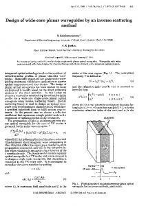
Fig. 1. Setup for Rmeas and Tmeas phantom measurements. The sphere is an 8-in. 共⬃20.3 cm兲 IS 080 SF from Labsphere, and the parameters are rbeam ⫽ 1 mm, dsample ⫽ 2.2 mm, dslide ⫽ 1 mm, rsample ⫽ 23 mm, rdetector ⫽ 12.5 mm, and ⫽ 633 nm. Note, during Rmeas measurements, the sample is placed at the port to the right-hand side.
cover the phantom optical property range sufficiently: 0 cm⫺1 ⱕ a ⱕ 3 cm⫺1, 4.4 cm⫺1 ⱕ ⬘s ⱕ 21.8 cm⫺1, g ⫽ 0.92, n ⫽ 1.33.
(6)
␦d rw , 1 ⫺ ␣w rw ⫺ ␣s rs ⫺ ␣d rd
(7)
where r denotes diffuse reflectance coefficients and ␣ denotes normalized areas relative to the total sphere area. The subscripts w, s, and d denote wall, sample, and detector, respectively. The initial reflected or transmitted intensity at the sample is P0 ⫽ rs Pin or P0 ⫽ ts Pin, respectively, where Pin is the intensity of the incident laser beam and rs and ts are diffuse reflectance and transmittance coefficients of the sample, respectively. Note that the specular reflectance Rspec leaves the sphere through the entrance port and that the collimated transmittance Tc ⬍⬍ Ttotal; thus both are ignored in this particular setup. To avoid direct exposure of the detector from P0, it was pulled back from the detector port; thus only diffuse reflectance from a portion of the opposite sphere wall was detected. The normalized area of this portion is denoted ␦d in Eq. 共7兲. Using a well-defined reflectance standard as a reference in conjunction with Eq. 共7兲, we extracted rs and ts from the phantom measurements and used these as input to the MPR method during the prediction analysis, i.e., Rmeas ⫽ rs and Tmeas ⫽ ts. 3. Results and Discussion
Except for the Monte Carlo simulations, all numerical analysis and algorithms in this paper were carried out with Matlab 5.2. Thus all matrix manipulation, least-squares fitting, etc., is based on standard Matlab routines. C.
Experimental Setup and Measurements
To carry out MPR tests on experimental data, we measured Rmeas and Tmeas of 20 liquid phantoms, each with a distinct set of a and ⬘s, using the integrating sphere setup shown in Fig. 1. The phantoms consisted of green food dye and 1.9-m polystyrene spheres suspended in water. During the measurements the phantoms were contained in cuvettes, consisting of two glass slides separated by a black plastic spacer. As illustrated in Fig. 1, some of the transmitted and reflected diffuse light is lost in real integrating sphere measurements, owing to the limited diameter of sample port. During the prediction analysis we therefore corrected Rsim and Tsim to take these transversal losses into account before the polynomial fits Rfit and Tfit were calculated. We did this by ignoring values of Rsim and Tsim for radial distances r ⬎ 0.5 rsample. Furthermore, we also had to carry out corrections due to losses through the ports and the reflective coating of the integrating sphere. The measured intensity at the detector Pout in an integrating sphere setup is the result of multiple reflections in the sphere originating from the first 1204
APPLIED OPTICS 兾 Vol. 39, No. 7 兾 1 March 2000
A.
Calibration Model
Figure 2 depicts the two simulated Rsim and Tsim data sets of the calibration model that we used in the MPR evaluations on simulated prediction data. As we stated above, the overall appearance of the Rsim and the Tsim plots is smooth and regular and thus well suited for polynomial fitting. Figure 3 shows the resulting fitting errors when two fifth-order double polynomials are used to fit the Rsim and Tsim plots in Fig. 2. The speckled appearance of the absolute error plots in Figs. 3共a兲 and 3共b兲 indicates that any systematic fitting errors due to the fitting algorithm are less significant than errors introduced by the random intrinsic noise of the Monte Carlo simulations. The relative errors of Rfit in Fig. 3共c兲 are significantly higher for low ⬘s values. This is because the low absolute levels of Rfit in this region 共see Fig. 2兲 are more easily afflicted by the Monte Carlo noise and that the applied least-squares regression algorithm optimizes the fit on the basis of the absolute—and not the relative— errors. Various preprocessing of Rsim and Tsim before fitting might reduce the latter error source. To test the performance of the Newton–Raphson algorithm separately, we also did predictions tests, using the original calibration data sets as input to the Newton–Raphson method, i.e., Rmeas ⫽ Rfit and Tmeas ⫽ Tfit. The results showed that the mean relative calculation error of both a and ⬘s was approximately 1 ⫻ 10⫺6. Furthermore, the Newton–
100 Rmeas and Tmeas data based on random a and ⬘s values within the ranges defined in relation 共5兲. Figure 4 shows the actual random distribution of a and ⬘s in the prediction set. All results discussed in the present subsection are based on this prediction set and the large 20 ⫻ 50 calibration set described in Subsection 2.B. Furthermore, all reported errors are relative prediction errors:
Err ⫽ 100%
冏
冏
pred ⫺ ref , ref
(8)
where pred is the predicted value and ref the true value of either a or ⬘s. The prediction errors of a or ⬘s are denoted Erra and Errs, respectively. 1. Order of Polynomials Table 1 gives the prediction errors using Rfit and Tfit fitting polynomials of orders 3, 4, and 5, respectively. The iterations of the Newton–Raphson algorithm were stopped when both ha and hs ⬍ 1 ⫻ 10⫺6 关see Eq. 共4兲兴. This criterion was typically satisfied after 5–15 iterations, leading to almost identical calculation times in all three cases. It is evident that the prediction accuracy of the fifth-order polynomials are superior to the third- and fourth-order polynomials. Sixth-order polynomials were also tested but caused rank deficient problems in the regression algorithm and were therefore rejected.
Fig. 2. Total diffuse reflectance R 共a兲 and transmittance T 共b兲 as a function of the absorption coefficient a and the reduced scattering coefficient ⬘s for a thin slab geometry. The R and T data for the plots were generated with Monte Carlo simulations.
Raphson algorithm converged in all cases; thus the specific contribution of the algorithm to the total prediction errors of the MPR method is negligible. B.
Numerical Prediction Tests
We tested the overall prediction performance of the MPR method, using a simulated prediction set of a
2. Large-Error Analysis The cases in which the prediction errors of a and兾or ⬘s, i.e., Erra and兾or Errs were larger than 0.5% with the fifth-order fits from Table 1 are depicted in Fig. 4. It appears that the Errs values are largest when R is low, whereas the largest Erra values occur mainly when R is low and T is high 共see discussion in subsection 3.A兲. To analyze the Monte Carlo noise contribution versus the fitting-error contribution to the total prediction error, we generated 10 identical but independent Rsim and Tsim sets for each of the 14 marked large-error cases in Fig. 4. The results from this analysis are shown in Fig. 5. In cases 1– 6 both Erra and Errs ⬎ 0.5% 共i.e., the triangles in Fig. 4兲, whereas in cases 7–14 only Errs ⬎ 0.5% 共i.e., the open circles in Fig. 4兲. In each of the 14 cases in Fig. 5 the left-hand bar indicates the maximum deviation from the true value, the middle bar is a measure of the prediction precision error, and the right-hand bar is a measure of the prediction accuracy error. By comparing the middle and the right-hand bars, we can conclude that the errors in cases 1– 6 are mainly due to MPR fitting errors in the calibration set, whereas the errors in cases 7–14 are not due to limitations of the MPR method in general but rather to the Monte Carlo noise in the prediction set. Thus only one of the latter eight cases were off by more than 0.5%, when we, in each case, calculated the mean of the ten independent predictions, i.e., the right-hand columns of Fig. 5. 1 March 2000 兾 Vol. 39, No. 7 兾 APPLIED OPTICS
1205
Fig. 3. 关共a兲 and 共b兲兴 Absolute and 关共c兲 and 共d兲兴 fitting errors of Rfit and Tfit.
3. Calculation Speed versus Accuracy The applied Newton–Raphson algorithm was implemented in Matlab and run on a 166-MHz Pentium personal computer. As shown in Table 1, one single prediction of a and ⬘s was calculated in ⬃60 ms. If the algorithms were implemented and compiled in,
Fig. 4. Solid curves, contour plots of constant Rsim and Tsim values as a function of a and ⬘s. The curves with positive slopes are Rsim plots, and the curves with negative slopes are Tsim plots. The markers depict the random distribution of a and ⬘s values in the simulated prediction set. The gray dots indicate cases with prediction errors less than 0.5%. The open circles are cases in which Errs exceeds 0.5%, and the triangles are cases in which both Erra and Errs exceed 0.5%. 1206
APPLIED OPTICS 兾 Vol. 39, No. 7 兾 1 March 2000
e.g., the C programming language, the calculations would run even faster. In contrast, it took days to generate the Monte Carlo data for the 20 ⫻ 50 calibration model we used. However, the total Monte Carlo calculation time may be reduced by means of either tracing less photons in each simulation or using less simulations to generate the calibration model. The calculation time might also be reduced with the Monte Carlo techniques suggested by Pifferi et al.20 Table 2 shows the resulting prediction errors of four equivalent fifth-order calibration models based on four Rsim and Tsim sets with two different numbers of simulations and two different numbers of photons per simulation. The results showed no significant increase in the mean prediction errors when either the number of photons or the number of simulations was reduced. Only when both the number of photons and the number of simulations were reduced simultaneously did a significant increase in the prediction errors occur. Consequently, the total calculation time of the calibration set may be reduced at least 10 times without any significant increase in the average prediction errors. 4. Similarity Principle When no collimated transmittance data Tc are available during integrating sphere measurements, the similarity principle is often assumed. However, this assumption is strictly valid only for large sample geometries and for g ⬎ 0.9.8 –10 We tested the validity of the similarity principle, using our calibration model 共 g ⫽ 0.9兲 on a series of simulated Rmeas and Tmeas with constant ⬘s but varying g. For constant ⬘s ⫽ 10 cm⫺1
Table 1. Prediction Errors, Number of Iterations, and Prediction Calculation Times for Polynomial Fits of Orders 3, 4, and 5
Erra 共%兲
Errs 共%兲
Orders
Mean
Max.
Mean
Max.
Iterations Mean
Calc. Time 共ms兲 Mean
Third order Fourth order Fifth order
1.0 0.4 0.2
7.8 3.1 1.4
0.8 0.4 0.3
6.2 3.5 1.1
11 11 11
54 56 60
we found that the prediction values of ⬘s deviated approximately ⫺2.5% at g ⫽ 0.8 and ⫹2.5% at g ⫽ 0.99, respectively. To determine g in conjunction with R and T measurements, it is necessary to perform Tc measurements also. Because of the practical difficulties involved in Tc measurements, the resulting measurement errors are often more severe than the errors arising from calibration models with a fixed g. However, the MPR method can be readily extended to include determination of s and g as well by generation of calibration models for various g values and application of a simple algorithm for choosing the appropriate model during each prediction. 5. Comparisons with other Methods We also compared the MPR method with the MCSI method5 and the IAD method.14 Both the latter
Fig. 5. Analysis of prediction errors greater than 0.5%. The upper graph 共a兲 shows Erra, and the lower 共b兲 shows the corresponding Errs. In each single case the three bars indicate the following: left, maximum deviation of ten identical simulations from the true value; middle, average deviation from the mean of the ten simulations; right, deviation of the mean of the ten simulations from the true value.
methods are capable of extracting the full set of optical properties, i.e., a, s, and g. To do this, they are designed to be fed with collimated transmittance data Tc in addition to the R and T data. In the case of the IAD method it is possible, though, to assume a g value and then use R and T data only. We chose to feed both the MCSI and the IAD method with Tc data calculated with the Beer–Lambert law and the Fresnel law. Table 3 shows the prediction errors, the prediction calculation time, and the number of outliers of the MPR, MCSI, and IAD methods, respectively. The outliers—which we defined as predictions with errors greater than 10%—were excluded from the mean prediction error calculations. All three methods were tested on the same computer. It appears that the MPR method is significantly faster and more accurate than both the IAD and the MCSI methods. As stated in Subsection 2.B, we applied a finite light source in these experiments. In fact, the IAD method implies uniform illumination; i.e., it is capable of handling one-dimensional light propagation only. This may to some degree account for the lower accuracy. Furthermore, we used only four quadrature points in the IAD calculations. Thus the accuracy of the IAD method may be improved by use of more quadrature points at the expense of the calculation speed. Although the MCSI and the MPR methods are both based on databases of Monte Carlo simulations, the MPR method yields significantly better accuracy and robustness than the MCSI method. This may be attributed to the fact that the MPR method is less sensitive to the Monte Carlo noise embedded in the databases. The MCSI method is based on spline interpolation of a selection of a few juxtaposed R or T points from the Monte Carlo database. Thus the MCSI fit will pass exactly through all of the selected data points and track any local variation, including intrinsic Monte Carlo noise. Owing to the local variability 共i.e., noise兲 in the Monte Carlo data 共see Fig. 3兲, the interpolated fit may even oscillate widely to pass
Table 2. Prediction Errors with Fifth-Order Polynomial Fits and a Reduced Number of Photon Packets and兾or Simulations for the Calibration Model
1 ⫻ 105 Photons兾Simulation Erra 共%兲
100 Simulations 1000 Simulations
1 ⫻ 106 Photons兾Simulation
Errs 共%兲
Erra 共%兲
Errs 共%兲
Mean
Max.
Mean
Max.
Mean
Max.
Mean
Max.
0.3 0.2
1.2 1.5
0.5 0.3
2.1 1.4
0.2 0.2
2.0 1.4
0.3 0.3
1.6 1.1
1 March 2000 兾 Vol. 39, No. 7 兾 APPLIED OPTICS
1207
Table 3. Prediction Errors, Prediction Calculation Times, and Number of Outliers
Methods
Erra 共%兲 Mean
Errs 共%兲 Mean
Calc. Time 共ms兲 Mean
Outliers 共%兲
MPR MCSI IAD
0.2 1.3 1.6
0.3 2.0 2.5
60 1350 350
0 9 9
through all data points and thereby produce unrealistic intermediate values. In contrast, the MPR method is based on two immediate fits including all R and T data points of the Monte Carlo database. In this case the fits are optimized with least-squares regression; thus any local variability in the R and T data will be smoothened out, which in turn will reduce the interference from the random Monte Carlo noise. C.
Phantom Measurements
To further validate the method, we also tested it on Rmeas and Tmeas data from phantom measurements. In these experiments we used the small 9 ⫻ 13 calibration set described in Subsection 2.C. Assuming that the scattering due to the dye in the phantoms was negligible, we determined the actual a of the 20 phantoms from collimated transmittance measurements of pure dye solutions, using the Beer–Lambert law. Also assuming that the absorption in the polystyrene spheres in the phantoms was negligible, we calculated the actual ⬘s of the phantoms, using Mie theory.21 Figure 6 shows correlation plots of the actual optical properties versus optical properties determined from integrating sphere measurements with the MPR method. In this case a few prediction outliers occurred when we used a fifth-order model, whereas a fourth-order model caused no such problems. This is probably because the higher-order models, although they are more accurate in general, may be more sensitive to the inevitable noise in measured prediction data and thus be less robust than lowerorder models. As a compromise between accuracy and robustness we therefore used fourth-order models for the predictions presented in Fig. 6. The means of Erra and Errs were 1.1% and 1.7%, respectively. In contrast to the errors reported in Subsection 3.B 共see Eq. 8兲, these errors are relative to the dynamic ranges of a and ⬘s in the phantoms: Err ⫽ 100%
冏
冏
pred ⫺ ref . ref,max ⫺ ref,min
(9)
We used the definition in Eq. 共9兲 in this case, because a includes zero values, leading to division by zero if Eq. 共8兲 is used instead. Although the prediction errors of the measurements are relatively small, they are slightly higher than the errors obtained from similar simulated tests on this model 共mean Erra ⬃ 0.7% and mean Errs ⬃ 0.2%兲. This is mainly due to uncertainties, partly in the determination of the exact sphere compensation parameters and partly in the 1208
APPLIED OPTICS 兾 Vol. 39, No. 7 兾 1 March 2000
Fig. 6. Correlation plots of theoretical calculations of a 共a兲 and ⬘s 共b兲 versus a and ⬘s values predicted by the MPR method from phantom measurements.
stated values of the applied optical properties of microspheres, glass, water, etc. Furthermore, the Monte Carlo simulations employ the Henyey– Greenstein phase function to calculate the scattering properties of the calibration data. However, the
Henyey–Greenstein phase function is an approximation to the more correct and complex phase function obtained from Mie theory calculations. Consequently, this may also account for some of the minor discrepancies between the predicted and the true values of a and ⬘s in Fig. 6. 4. Conclusions
The above results show that the MPR method is accurate, fast, and robust. The minor increase in the prediction errors for low-reflectance levels may be reduced by preprocessing of the calibration data before the fitting is performed. However, if this particular region is of main interest, it would be better to apply a larger sample thickness to increase the reflectance signal level and thereby reduce the effect of the interference from Monte Carlo noise and measurement noise. It appears that the similarity principle is not strictly valid in the above experiments. Consequently, g variations lead to increased but systematic ⬘s prediction errors of the MPR method. However, if necessary, the MPR method could readily be extended to include direct determination of s and g as well, and thus circumvent any similarity problems. The calculations of the data for the calibration model suffer from the same advantages and drawbacks as all other Monte Carlo-based methods. The main advantages are the flexibility in sample geometry and the potentially high accuracy. The major drawback is the calculation time needed to obtain this high accuracy. However, the results showed that the MPR method maintained a high level of accuracy when the number of simulations or traced photons in the calibration data set was significantly reduced, i.e., 10 times. In our case this meant that the calculation time of the calibration data could be reduced from days to hours. The predicted values of a and ⬘s with the MPR method on data from real integrating sphere measurements showed good correlation with theoretically calculated values. These experiments also showed that, when MPR predictions involve real measurement data, it is essential to include proper compensation for the various radiation losses in the setup. Furthermore, it may be necessary to decrease the order of the polynomial fits to obtain robust results on measured 共i.e., noisy兲 data compared with similar experiments on simulated data. In conclusion, it is evident that, once the calibration model has been implemented, the prediction speed, the accuracy, and the robustness of the MPR method is sufficient for a wide range of real-time spectroscopic analysis applications with integrating sphere measurements. The authors acknowledge the financial support from the Danish Academy of Technical Sciences. References 1. N. M. Anderson and P. Sekelj, “Light-absorbed and scattering properties of non-haemolysed blood,” Phys. Med. Biol. 12, 173– 184 共1967兲.
2. A. M. K. Nilsson, G. W. Lucassen, W. Verkruysse, S. Andersson-Engels, and M. J. C. van Gemert, “Changes in optical properties of human whole blood in vitro due to slow heating,” Photopchem. Photobiol. 65, 366 –373 共1997兲. 3. A. Roggan, M. Friebel, K. Do¨rschel, A. Hahn, and G. Mu¨ller, “Optical properties of circulating human blood in the wavelength range 400 –2500 nm,” J. Biomed. Opt. 4, 36 – 46 共1998兲. 4. A. N. Yaroslavsky, I. V. Yaroslavsky, T. Goldback, and H.-J. Schwarzmaier, “Influence of the scattering phase function approximation on the optical properties of blood determined from the integrating sphere measurements,” J. Biomed. Opt. 4, 47–53 共1998兲. 5. A. M. K. Nilsson, R. Berg, and S. Andersson-Engels, “Measurements of the optical properties of tissue in conjunction with photodynamic therapy,” Appl. Opt. 34, 4609 – 4619 共1995兲. 6. W.-C. Lin, M. Motamedi, and A. J. Welch, “Dynamics of tissue optics during laser heating of turbid media,” Appl. Opt. 35, 3413–3420 共1996兲. 7. A. J. Welch, M. J. C. van Gemert, W. M. Star, and B. C. Wilson, “Overview of tissue optics,” Optical-Thermal Response of Laser-Irradiated Tissue, A. J. Welch and M. J. C. van Gemert, eds. 共Plenum, New York, 1995兲, Chap. 2. 8. H. C. van de Hulst, Multiple Light Scattering, Vols. I and II 共Academic, New York, 1980兲. 9. R. Graff, J. G. Aarnoudse, F. F. M. de MulHenk, and W. Jentink, “Similarity relations for anisotropic scattering in absorbing media,” Opt. Eng. 32, 244 –252 共1993兲. 10. D. R. Wyman, M. S. Patterson, and B. C. Wilson, “Similarity relations for anisotropic scattering in Monte Carlo Simulations of deeply penetrating neutral particles,” J. Comp. Physiol. 81, 137–150 共1989兲. 11. J. W. Pickering, S. A. Prahl, N. van Wieringen, J. B. Beek, H. J. C. M. Sterenborg, and M. J. C. van Gemert, “A double integrating sphere system for measuring the optical properties of tissue,” Appl. Opt. 32, 399 – 410 共1993兲. 12. P. Kubelka, “New contributions to the optics of intensely light scattering materials. Part I,” J. Opt. Soc. Am. A 4, 448 – 457 共1948兲. 13. J. Reichmann, “Determination of absorption and scattering coefficients for nonhomogeneous media. 1. Theory,” Appl. Opt. 12, 1811–1815 共1973兲. 14. S. A. Prahl, M. J. C. van Gemert, and A. J. Welch, “Determining the optical properties of turbid media by using the adding– doubling method,” Appl. Opt. 32, 559 –568 共1993兲. 15. C. R. Simpson, M. Kohl, M. Essenpreis, and M. Cope, “Near Infrared optical properties of ex-vivo human skin and subcutaneous tissues measured using the Monte Carlo inversion technique,” Phys. Med. Biol. 43, 2465–2478 共1998兲. 16. L.-H. Wang, S. L. Jacques, and L.-Q. Zheng, “MCML—Monte Carlo modeling of photon transport in multi-layered tissues,” Comput. Methods Programs Biomed. 47, 131–146 共1995兲. 17. S. V. Chapra and R. P. Canale, Numerical Methods for Engineers 共McGraw-Hill, New York, 1997兲, Chap. 6. 18. W. F. Cheong, S. A. Prahl, and A. J. Welch, “A review of the optical properties of biological tissue,” IEEE J. Quantum Electron. 26, 2166 –2185 共1990兲. 19. J. F. Beek, P. Blokland, P. Posthumus, M. Aalders, J. W. Pickering, H. J. C. M. Sterenborg, and M. J. C. van Gemert, “In vitro double-integrating-sphere optical properties of tissues between 630 and 1064 nm,” Phys. Med. Biol. 42, 2255–2261 共1997兲. 20. A. Pifferi, P. Taroni, G. Valentini, and S. Andersson-Engels, “Real-time method for fitting time-resolved reflectance and transmittance measurements with a Monte Carlo model,” Appl. Opt. 37, 2774 –2780 共1998兲. 21. C. F. Bohren and D. R. Huffman, Absorption and Scattering of Light by Small Particles 共Wiley, New York, 1983兲.
1 March 2000 兾 Vol. 39, No. 7 兾 APPLIED OPTICS
1209