[3] A. Girard, C.E. Rasmussen, and R. Murray-Smith. Gaussian process priors with uncertain inputs: Multiple-step ahead prediction. Technical Report 119, Dept.
Multiple-step Time Series Forecasting with Sparse Gaussian Processes Perry Groot ab
Peter Lucas a
Paul van den Bosch b
a
Radboud University, Model-Based Systems Development, Heyendaalseweg 135, 6525 AJ Nijmegen b Technical University Eindhoven, Department of Electrical Engineering, Control Systems, Potentiaal 4.28, 5600 MB Eindhoven Abstract Forecasting of non-linear time series is a relevant problem in control. Furthermore, an estimate of the uncertainty of the prediction is useful for constructing robust controllers. Multiple-step ahead forecasting has recently been addressed using Gaussian processes, but direct implementations are restricted to small data sets. In this paper we consider multiple-step forecasting for sparse Gaussian processes to alleviate this problem. We derive analytical expressions for multiple-step ahead prediction using the FITC approximation. On several benchmarks we compare the FITC approximation with a Gaussian process trained on a large portion of randomly drawn training samples. As a consequence of being able to handle larger data sets, we show a mean prediction that is closer to the true system response with less uncertainty.
1
Introduction
In this paper we consider non-linear time series of the form xt+1 = f (xt , ut ),
yt = xt + �t
(1)
with t a time index, x the system state, u a controllable input, y the observed state, � ∼ N (0, σ 2 ) a noise term, and f some non-linear transition function. In particular we consider the problem of forecasting future states, which is a relevant problem in control. Forecasting allows one to choose controls u in order to optimize a predefined economic criteria, for example, the throughput and amount of power used by a printer while print quality remains high. In this paper we focus on forecasting using a Gaussian process (GP), a flexible Bayesian framework that places a prior distribution over functions. The GP provides both a mean and a variance for each prediction, which is useful for constructing robust controllers [7, 12]. Multiple-step forecasting can be done using direct forecasting or using iterative one-step predictions with the latter usually being superior [2]. A naive way of repeatedly doing one-step ahead predictions is to feed back the mean of the prediction into the system state, but this has been shown to severely underestimate the uncertainty of the model predictions. A better approach is to also take the uncertainty of the input of the ith step into account to compute the (i + 1)th step predictive distribution. The details using a Gaussian process (GP) approach have been worked out in [3, 4, 8, 9]. Initially by using Taylor approximations [3], but later extended to exact expressions for the first and second moments of the predictive distribution [8, 9], which can be solved analytically for a number of covariance functions [9, 5, 1]. Although for non-linear dynamical systems, a Gaussian input distribution does not guarantee the predictive distribution to be Gaussian, a GP allows an analytic Gaussian approximation that uses exact moment matching which has been shown to correspond well to the gold standard of MCMC sampling. A direct implementation of GPs, however, limits their applicability to small data sets since the kernel matrix needs to be stored, costing O(N 2 ), and inverted, costing O(N 3 ), with N the number of data points. In recent years several approaches have addressed this problem often selecting a subset of the training data (the active set) of size M reducing the computational complexity to O(M 2 N ) for M � N . In this paper we
focus on the FITC approximation [13], one of the leading methods for modeling sparse GPs, which relaxes the constraint that the active set has to come from the training data. This allows the M pseudo-inputs and addtional hyperparameters to be optimized at the same time. The contribution of this paper are analytical expressions for multiple-step ahead prediction using the FITC approximation. We obtain a method with a predictive model that executes several magnitudes faster than the standard GP. On several benchmarks we compare the FITC approximation with a GP trained on a large portion of randomly drawn training samples. As a consequence of being able to handle larger data sets, we also show a mean prediction that is closer to the true system response with less uncertainty. The rest of this paper is structured as follows. Section 2 describes background information on Gaussian process regression and the FITC approximation for sparse GPs. Section 3 describes iterative one-step ahead time series forecasting using uncertainty propagation. Section 4 derives the analytical equations for time series forecasting with the FITC approximation. Section 5 presents two illustrative examples. Section 6 summarizes our conclusions.
2
Sparse Gaussian process regression
We denote vectors x and matrices K with bold-face type and their components with regular type, i.e., xi , Kij . With xT we denote the transpose of the vector x. N (x|m, V ) is a Gaussian distribution with mean m and covariance V .
2.1
Gaussian processes
In this section we briefly describe the Gaussian process model for regression [11]. Let D be a data set consisting of N observed D-dimensional input vectors X = {xn }N n=1 and corresponding real-valued outputs y = {yn }N n=1 . We assume that function observations follow from a latent function f that are corrupted by additive iid zero mean Gaussian noise, i.e., y = f (x) + � with � ∼ N (0, σ 2 ). We place a GP prior on the latent function f giving a multi-variate Gaussian distribution on any finite subset of latent variables, i.e., the values of the function f (x) at location x. The GP is completely specified by a mean function (typically taken to be zero) and covariance function. In particular we have p(f |X) = N (f |0, KN N ) where the covariance matrix KN N is constructed from the covariance function [KN N ]nn0 = K(xn , xn0 ). Typically the covariance function depends on additional hyperparameters. In this paper we will make use of the squared exponential (SE) covariance function with automatic relevance determination (ARD) hyperparameters � � 1 T −1 (2) K(xn , xn0 ) = v exp − (xn − xn0 ) W (xn − xn0 ) 2 2 where W = diag(w12 , . . . , wD ) allows for different length scales along each input dimension and v specifies the signal variance. By integrating out the latent function values we obtain the marginal likelihood
p(y|X, Θ) = N (y|0, KN N + σ 2 I)
(3)
with Θ = {v, w1 , . . . , wD , σ 2 } all hyperparameters which we usually omit for readability. Maximum likelihood estimates for Θ are typically obtained by minimizing the negative log marginal likelihood (e.g., using gradient descent), which can be evaluated exactly in the case of GP regression and is given by [11] − log p(y|X) =
1 T 1 N y (KN N + σ 2 I)−1 y + log |KN N + σ 2 I| + log(2π). 2 2 2
(4)
The predictive distribution is obtained by considering a new point x∗ and conditioning on the hyperparameters Θ and data D, which gives p(y|x∗ , D, Θ) = N (y|µ∗ , σ∗2 ) with µ∗ = K∗N (KN N + σ 2 I)−1 y,
σ∗2 = K∗∗ − K∗N (KN N + σ 2 I)−1 KN ∗ + σ 2
(5)
Gaussian processes do not scale well for large data sets since training requires O(N 3 ) time because of the inversion of the covariance matrix. Once the inversion is done, computing the predictive mean is O(N ) and computing the predictive variance is O(N 2 ) per new test case.
2.2
Sparse Gaussian processes
In this section we briefly describe the sparse pseudo-input Gaussian process [13], which was later renamed to Fully Independent Training Conditional (FITC) model to fit in the systematic framework of [10]. The ¯ = {x ¯ m }M FITC model approximates the full GP using M pseudo-inputs X m=1 that are not restricted to the data inputs, but are rather hyperparameters that can be learned. Given a base covariance function K, the FITC covariance function has the following form: −1 K F IT C (xn , xn0 ) = KnM KM M KM n0 + λn δnn0 ,
−1 λn = Knn − KnM KM M KM n
(6)
¯ m ) of covariances between data inputs and pseudo-inputs where KnM is the matrix with elements K(xn , x ¯m, x ¯ m0 ) of covariances between pseudo-inputs. The marginal and KM M is the matrix with elements K(x likelihood is similar to Eq. (3) ¯ Θ) = N (y|0, K F IT C + σ 2 I) p(y|X, X, NN
(7)
which is used analogous to Eq. (4) to learn hyperparameters and pseudo-inputs of the FITC model jointly by minimizing the negative log likelihood using gradient descent. The predictive distribution is computed just as the standard GP model by considering a new point x∗ and conditioning on the data D giving ¯ Θ) = N (y|µ∗ , σ 2 ) with p(y|x∗ , D, X, ∗ µ∗ = K∗M Q−1 KM N (Λ + σ 2 I)−1 y,
−1 −1 σ∗2 = K∗∗ − K∗M (KM )KM ∗ + σ 2 M −Q
(8)
where Q = KM M + KM N (Λ + σ 2 I)−1 KN M and Λ = diag(λ). F IT C (cf. Training the FITC model is computationally more efficient since the covariance matrix KN N Eq. (6)) consists of a sum of a low rank part and a diagonal part and can therefore be inverted in O(M 2 N ) rather than O(N 3 ). After some precomputations, computing the predictive mean is O(M ) and computing the predictive variance is O(M 2 ) per new test case.
3
Iterative time-series forecasting with uncertainty propagation
In this section we briefly review iterative one-step ahead prediction with uncertainty propagation [3, 4, 8, 9]. We assume an autoregressive Gaussian process model with L lagged outputs given by xk = [yk−L , . . . , yk−1 ]T ,
yk = f (xk ) + �
(9)
with f some non-linear function and � ∼ N (0, σ 2 ) a white noise term. Assuming the time series is known up to time T , denoted by YT , predicting the system k-steps ahead at time T +k can be achieved by repeatedly doing one-step ahead predictions. When the input is a random variable x∗ with an input distribution given by p(x∗ |u, S) ∼ N (u, S), the predictive distribution of the function value p(f∗ ) is obtained by integrating over the input distribution: Z p(f∗ |u, S, D) = p(f∗ |x∗ , D)p(x∗ |u, S) dx∗ (10) The idea of iterative one-step ahead prediction with uncertainty propagation is to approximate at each step t the predictive distribution with a Gaussian distribution N (m(ut , St ), v(ut , St )). It has been shown that the first and second moment of the predictive distribution can be computed analytically for the SE kernel (cf. Eq. (2)) giving a prediction p(yt |YT ) ∼ N (m(ut , St ), v(ut , St ) + σ 2 ), which is then fed back into the system state and represented by N (m(ut+1 , St+1 ), v(ut+1 , St+1 )). In particular, at time T + 1 we have yT +1−L 0 ... 0 . .. .. uT +1 = (11) and ST +1 = .. . . yT
0
...
0
Since p(yT +1 |YT ) ∼ N (m(uT +1 , ST +1 ), v(uT +1 , ST +1 ) + σ 2 ) we have at time T + 2: yT +2−L 0 ... 0 . .. . .. uT +2 = and ST +2 = .. . m(uT +1 , ST +1 )
0
...
v(uT +1 , ST +1 ) + σ
2
(12)
This is repeated iteratively until at time T + k we have m(uT +k−L , ST +k−L ) .. uT +k = and .
ST +k
4
m(uT +k−1 , ST +k−1 ) v(uT +k−L , ST +k−L ) + σ 2 .. = . cov(yT +k−1 , yT +k−L )
... ...
cov(yT +k−L , yT +k−1 ) .. . 2 v(uT +k−1 , ST +k−1 ) + σ
(13)
Time series forecasting with sparse GPs
In this section we will derive the mathematical equations necessary for multiple-step ahead prediction with the FITC covariance function described in Section 2.2. In order to use the multiple-step ahead prediction approach described in Section 3, we need expressions for the mean m(ut , St ), variance v(ut , St ) and −1 −1 covariance cov(yt , yt0 ). Let B (1) = Q−1 KM N (Λ + σ 2 I)−1 y and B (2) = KM . The predictive M −Q (1) equations using the FITC Gaussian process model are then given by µ(x∗ ) = K∗M B and σ∗2 = K∗∗ − K∗M B (2) KM ∗ + σ 2 . Furthermore, we define the following quantities for a kernel K: R (1) Li = K(x∗ , xi )p(x∗ ) dx∗ R (3) Li = x∗ K(x∗ , xi )p(x∗ ) dx∗
R (2) Lij = K(x∗ , xi )K(x∗ , xj )p(x∗ ) dx∗ R L(4) = K(x∗ , x∗ )p(x∗ ) dx∗
(14)
Thus L(1) is a N × 1 vector, L(2) a N × N matrix, L(3) a N × D matrix, and L(4) a scalar with N the number of training data points and D the dimension of the data. In [9] it has been shown that for the SE kernel (cf. Eq. (2)) the expressions m(ut , St ), v(ut , St ), and cov(yt , yt0 ) can be stated in terms of L(1) , . . . , L(4) which can be solved analytically: (1)
Li (2) Lij (3)
Li L(4)
� = v|W −1 S + I|−1/2 exp − 12 (u − xi )T (S + W )−1 (u − xi ) = v 2 |2W −1� S + I|−1/2 �� −1 exp − 21 (u − xd )T ( W (u − xd ) + (xi − xj )T (2W )−1 (xi − xj ) 2 + S) (1) = Li ci =v
(15)
where xd = 12 (xi + xj ) and ci = (W −1 + S −1 )−1 (W −1 xi + S −1 u). In the remainder we derive analytical expressions for the mean m(ut , St ), variance v(ut , St ) and covariance terms cov(yt , yt0 ) for the FITC kernel function with respect to some base kernel K. We omit the time index t for brevity. Since the predictive mean is given by µ(x∗ ) = K∗M B (1) it holds that Z Z X (1) ¯ m )p(x∗ ) dx∗ m(u, S) = Ex∗ [µ(x∗ )] = µ(x∗ )p(x∗ ) dx∗ = Bm K(x∗ , x
Computing the mean.
(16)
m
P (1) (1) Thus m(u, S) = m Bm Lm = (B (1) )T L(1) where L(1) is the required integral for the base kernel K with respect to the pseudo-inputs.
Computing the variance. Since v(u, S) = Ex∗ [σ 2 (x∗ )] + Ex∗ [µ(x∗ )2 ] − Ex2 ∗ [µ(x∗ )]. These three terms give respectively Z � � Ex∗ [σ 2 (x∗ )] = K(x∗ , x∗ ) − K∗M B (2) KM ∗ p(x∗ ) dx∗ XXZ X X (2) (2) (2) (4) ¯ i )Bij K(x∗ , x ¯ j )p(x∗ ) dx∗ = L(4) − =L − K(x∗ , x Bij Lij i
j
i
j
Z X (1) ¯ i ))2 p(x∗ ) dx∗ Ex∗ [µ(x∗ )2 ] = ( Bi K(x∗ , x
(17)
i
= Ex2 ∗ [µ(x∗ )]
XX
=(
(1)
(1)
Z ¯ i )K(x∗ , x ¯ j )p(x∗ ) dx∗ = K(x∗ , x
Bi Bj
i
j
X
(1) (1) Bi Li )2
XX i
(1)
(1)
(2)
Bi Bj Lij
j
i
Thus we obtain the following expression for the variance X X (2) X (1) (1) (1) (1) (2) v(u, S) = L(4) − (Bij − Bi Bj )Lij − ( Bi Li )2 i (4)
=L
j
�
− Tr (B
i (2)
−B
(1)
(B
(1) T
) )L
(2)
�
(18)
� � − Tr B (1) (B (1) )T L(1) (L(1) )T
Computing the covariances. For the covariance terms we compute cov(yt , xt ). The needed covariances can then be obtained by removing the oldest element of the state vector xt . Omitting the time index, it holds that cov(y, x) = E[yx] − E[y]E[x] where E[y] = m(u, S) and E[x] = u. Since Z E[yx] = xµ(x)p(x) dx Z (19) X X (1) (1) (3) ¯ m )p(x) dx = = Bm xK(x, x Bm Lm m
m
we obtain the following expression for the covariance terms X X (1) (3) (1) (1) cov(y, x) = Bm Lm − ( Bm Lm )u m
(20)
m
In the next section we present experimental results for multiple-step ahead prediction for two benchmark problems leading to a better predictive distribution when using the FITC approximation compared to a standard GP. At the same time computing the predictive distribution is more efficient since the expressions ¯ = {x ¯ m }M L(1) , . . . , L(4) are computed for the base kernel K with respect to the pseudo-inputs X m=1 . Thus (1) (2) (3) (4) L is a M × 1 vector, L a M × M matrix, L a M × D matrix, and L a scalar with M the number of pseudo-inputs and D the dimension of the data.
5
Experiments
In this section we compare the FITC model with a standard GP model on two benchmark problems. We report the mean together with their 2σ error bars. To evaluate the goodness of fit of the model we also report the root mean squared error (RMSE) and the absolute mean error (MAE). The RMSE is defined as v u N u1 X (yi − yˆi )2 , (21) RM SE = t N i where yi is the target value, yˆi predicted value, and N the number of test examples. Since the RMSE can be dominated by a few large residuals we also report the MAE which is defined as M AE = in which the influence of individuals is linear.
N 1 X |yi − yˆi |, N i
(22)
Example 1. The first benchmark that we consider is a simple dynamical system with one system state and one control input given by xk+1 = 0.95 ∗ tanh(xk ) + sin(uk ),
yk = xk + �k
(23)
where at time k, xk is the system state, uk is the known control input, and �k ∼ N (0, σ 2 ) is a noise term. We generated time series data of 1000 points used for training. Given values yk , uk for k = 1, . . . , 1000 we generated a training data set of the form y2 y1 u1 y3 y2 u2 (24) Y = . X= . . .. .. .. y1000 y999 u999 We trained a GP model with a squared exponential kernel as in Eq. (2) on N = 200 points randomly drawn training data points. The sparse GP model used a squared exponential base kernel and was trained using all training data and M = 20 pseudo-inputs. Figure 1 shows the mean prediction and 2σ error bars of both models from k = 1 to k = 100 steps ahead on a separate test set. In the training data the control signal ranged between −2 and 2 whereas in the test set the control signal ranged between −3 and 3 explaining the higher amount of uncertainty whenever |uk | > 2 occurs. The sparse GP model shows a mean prediction that is closer to the true model with less uncertainty. The RMSE and MAE are reported in Table 1 showing slightly better values for the FITC model. The FITC model is, however, much more efficient for multiplestep ahead prediction since M � N . 3
3 ± 2σ mean true control
2
± 2σ mean true control
2
1
1
0
0
−1
−1
−2
−2
−3
−3 0
20
40
60
80
100
0
20
40
60
80
100
Figure 1: Dynamic system 100-step ahead prediction benchmark. Left: standard GP using 200 randomly drawn training inputs. Right: FITC with 20 pseudo-inputs.
Table 1: Comparison for two multiple-step ahead prediction benchmarks. Example 1 Example 2 GP FITC GP FITC RMSE 0.55 0.54 0.34 0.09 MAE 0.37 0.35 0.26 0.06
Example 2. A well-known benchmark for multiple-step ahead prediction is the Mackey-Glass chaotic z(t−τ ) time series, defined as dz(t) dt = −bz(t) + a 1+z(t−τ )10 , which shows strong non-linear behaviour [6]. In our experiments we used a = 0.2, b = 0.1, and τ = 17 and the resulting time series was re-sampled with period 1 and normalized. For the models we used 16 lagged outputs in the state vector xk = [yk−16 , . . . , yk−1 ] where yk is the observed system state xk corrupted by white noise with variance 0.001.
We trained a GP model with a squared exponential kernel as in Eq. (2) on N = 200 points randomly drawn from a time series of 1200 points. The sparse GP model used a squared exponential base kernel and was trained using the 1200 points and M = 40 pseudo-inputs. Figure 2 shows the mean prediction and two standard deviations of both models from k = 1 to k = 100 steps ahead on a separate test set. The sparse GP model clearly shows a mean prediction that is closer to the true model with less uncertainty. At the same time the k-step ahead prediction is much more efficient since M � N . The RMSE and MAE are reported in Table 1, showing much beter values for the FITC model. 2
2 ± 2σ mean true
1.5
± 2σ mean true
1.5
1
1
0.5
0.5
0
0
−0.5
−0.5
−1
−1
−1.5
−1.5
−2
−2
−2.5
−2.5
−3
−3 0
20
40
60
80
100
0
20
40
60
80
100
Figure 2: Mackey-Glass 100-step ahead prediction benchmark. Left: standard GP using 200 randomly drawn training inputs. Right: FITC with 40 pseudo-inputs.
6
Conclusions
In this paper we looked at the problem of non-linear time series forecasting in the context of iterative onestep predictions. A naive approach that only propagates the mean of the predictive distribution typically underestimates the uncertainty of the model predictions. This can be improved by also taking the uncertainty of the input into account. Details of such an approach has been worked out earlier using Gaussian processes. Naive implementations of Gaussian processes, however, limits their applicability to small data sets since inverting the kernel matrix costs O(N 3 ) with N the number of data points. In this paper we have derived analytical equations for multiple-step ahead forecasting using sparse Gaussian processes. We reported results on two dynamical systems examples between a standard GP and a sparse GP. The sparse GP approach produced results several magnitudes faster than the standard GP approach. As a consequence of being able to handle larger data sets this also resulted in better predictive distributions. Further research will focus on extending the presented framework for forecasting using sparse GPs with dimensionality reduction [14] and control optimization [12]. Other interesting directions are to combine the problem of predicting from noisy inputs with the problem of training a model from noisy inputs.
Acknowledgement This work has been carried out as part of the OCTOPUS project with Oc´e Technologies B.V. under the responsibility of the Embedded Systems Institute. This project is partially supported by the Netherlands Ministry of Economic Affairs under the Bsik program.
References [1] K. Aˇzman and J. Kocijan. Non-linear model predictive control for models with local information and uncertainties. Transactions of the Institute of Measurement and Control, 30(5):371–396, 2008.
[2] J.D. Farmer and J.J. Sidorowich. Exploiting chaos to predict the future and reduce noise. Technical Report LA-UR-88, Los Alamos National Laboratory, 1985. [3] A. Girard, C.E. Rasmussen, and R. Murray-Smith. Gaussian process priors with uncertain inputs: Multiple-step ahead prediction. Technical Report 119, Dept. of Computing Science, University of Glasgow, 2002. [4] A. Girard, C.E. Rasmussen, J. Qui˜nonero-Candela, and R. Murray-Smith. Gaussian process priors with uncertain inputs - application to multiple-step ahead time series forecasting. In Neural Information Processing Systems, 2003. [5] J. Kocijan, A. Girard, and D.J. Leith. Incorporating linear local models in Gaussian process model. Technical Report IJS report DP-8895, Jozef Stefan Institute, 2004. [6] M.C. Mackey and L. Glass. Oscillation and chaos in physiological control systems. Science, 197:287– 289, 1977. [7] R. Murray-Smith and D. Sbarbaro. Nonlinear adaptive control using non-parametric Gaussian process prior models. In 15th IFAC World Congress on Automatic Control, 2002. [8] J. Qui˜nonero-Candela, A. Girard, J. Larsen, and C.E. Rasmussen. Propagation of uncertainty in Bayesian kernel models - application to multiple-step ahead forecasting. In International Conference on Acoustics, Speech and Signal Processing, volume 2, pages 701–704, Hong-Kong, 2003. IEEE. [9] J. Qui˜nonero-Candela, A. Girard, and C.E. Rasmussen. Prediction at an uncertain input for Gaussian processes and relevance vector machines - application to multiple-step ahead time-series forecasting. Technical report, IMM, Danish Technical University, 2002. [10] J. Qui˜nonero-Candela and C.E. Rasmussen. A unifying view of sparse approximate Gaussian process regression. Journal of Machine Learning Research, 6:1939–1959, 2005. [11] C.E. Rasmussen and C.K.I. Williams. Gaussian processes for machine learning. MIT Press, Cambridge, MA, 2006. [12] D. Sbarbaro and R. Murray-Smith. Self-tuning control of non-linear systems using gaussian process prior models. Lecture Notes in Computer Science, 3355:140–157, 2005. [13] E. Snelson and Z. Ghahramani. Sparse Gaussian processes using pseudo-inputs. In Advances in Neural Information Processing Systems. MIT Press, 2006. [14] E. Snelson and Z. Ghahramani. Variable noise and dimensionality reduction for sparse Gaussian processes. In Proceedings of the 22nd Annual Conference on Uncertainty in AI. AUAI Press, 2006.