pareto distribution (GPD) arises as the limiting distribution. The concept of .... standard normal cumulative distributi
50th AIAA/ASME/ASCE/AHS/ASC Structures, Structural Dynamics, and Materials Conference
17th 4 - 7 May 2009, Palm Springs, California
AIAA 2009-2256
Conservative Reliability Estimates in Design Optimization Using Multiple Tail Median Palaniappan Ramu1 Dept. of Aerospace & Mechanical Engineering, University of Notre Dame, Notre Dame, IN 46556 Nam H. Kim2 and Raphael T. Haftka3 Dept. of Mechanical & Aerospace Engineering, University of Florida, Gainesville, FL 32611, USA
Inevitable uncertain and/or random variables call for probabilistic approaches in design optimization. Sampling based reliability estimation in such approaches is computationally expensive when designing for high reliability. When available samples are scarce, techniques like tail models are widely used to extrapolate reliability levels from observed levels to unobserved levels. One such approach, the multiple tail median uses a suite of tail models to estimate reliability in the performance space. The method provides the median as the compromise estimate and an insurance against worst predictions. This work associates ranks to the estimates and uses the estimate that is ranked higher than the median as a conservative estimate for reliability.
Nomenclature D D0 E FG ( g )
FG (u ) Fu(z) Fˆ , ( z )
= Tip displacement = Allowable deflection = Young’s Modulus = CDF of G
= CDF of G at u = Conditional CDF = Approximated conditional CDF
FX
= Load in X direction
FY G Gd Gp Gs gc gr L N Nex Pi p Pf R Sr t u
= Load in Y direction = Performance measure = Displacement performance measure = (p×N)th quantile of G = Stress performance measure = Capacity = Response = Length = Total number of samples = Number of exceedances (samples in tail region) = Empirical CDF = Probability = Failure probability = Yield strength = reciprocal of conventional safety factor = thickness = threshold for samples assumed to lie in tail region
1
Postdoctoral Research Associate, AIAA member Associate Professor, AIAA Member 3 Distinguished Professor, AIAA Fellow 2
1 American Institute of Aeronautics and Astronautics Copyright © 2009 by Palaniappan Ramu. Published by the American Institute of Aeronautics and Astronautics, Inc., with permission.
w z
comp
Beta-LT Beta-QH GPD LnBeta-QT ML MTM Reg
= width = exceedance = Reliability index = Shape parameter = Computed stress = Standard normal cumulative distribution function (CDF) = Scale parameter = Fit a linear polynomial to the tail data Inverse normal cumulative distribution function applied to the CDF of Sr = Fit a quadratic polynomial to half of the data. Inverse normal cumulative distribution function applied to the CDF of Sr = Generalized Pareto Distribution = Fit a Quadratic polynomial to the tail data. Logarithmic transformation applied to the beta transformed CDF = Maximum Likelihood = Multiple Tail Median = Regression
Introduction
I
nspite of the prohibitive computational expense, simulation approaches like Monte Carlo Simulation (MCS) are widely used for reliability estimation. Among the several advantages that MCS features, the ability to handle multiple failure modes and complex limit states unlike analytical approaches is attractive for reliability estimation context. Since reliability analysis is an iterative process and using MCS is computationally prohibitive, researchers develop variants of MCS or other approximation methods like response surface or surrogate metamodels that replace the expensive simulations. High reliability translates to small probability of failure, determined by the tails of the statistical distributions. Since the safety levels can vary by an order of magnitude with slight modifications in the tails of the response variables1, the tails need to be modeled accurately. Application of crude MCS is tedious not feasible if not impossible. Therefore, extrapolation techniques can be used. Statistical techniques from extreme value theory (referred to as classical tail modeling techniques here) are available to perform this extrapolation. The basic idea in tail modeling techniques is to approximate the conditional cumulative distribution function (CDF) above a certain threshold by the Generalized Pareto Distribution2 (GPD). In order to do this, one needs to estimate the parameters of GPD. There are several competing methods available for parameter estimation. This paper uses the maximum likelihood and least square regression techniques. The multiple tail median approach (MTM) uses five different data fitting techniques. In addition to the GPD based techniques, it uses three alternate extrapolation techniques in the performance space. The alternate techniques are based on the idea of approximating the relationship between the performance measure and the transformed CDF. A nonlinear transformation is applied to the CDF and the first technique approximates about the top 10% of data using a linear polynomial. The second technique approximates the upper half of the transformed CDF by a quadratic polynomial. The third technique applies a logarithmic transformation to the already transformed CDF and approximates the tail with a quadratic polynomial. It is to be noted that all five techniques do not approximate the functional expression of the model output; rather they approximate the tail of CDF. Thus, they do not need to be tailored to any functional form of the output. The MTM applies all the techniques simultaneously and use the median of the five estimates as the best estimate. The MTM provides a compromise estimate using few samples but it is very dependent on the noise in the initial native sample. This noise is inherent of the volatile CDF tails. Therefore, a measure of how much one can trust the MTM is desirable. It was shown that the range of the five estimates can be used to approximate the error associated with the MTM18. However, it was not very clear by how much the range does over or under estimate the error which might lead to overly conservative designs. Here, an efficient statistical technique called bootstrap is used to compute the confidence bounds on the MTM. Often times a designer settles for a conservative design than an optimal design that can fluctuate around exact value. Therefore, it is explored whether the upper bound of the confidence interval can be used as a conservative estimate for the MTM. It is observed that though bootstrap can provide confidence bounds, the upper bounds are not always necessarily conservative. 2 American Institute of Aeronautics and Astronautics
Individual estimates from the suite of tail models can be grouped into equal sized bins and ranks assigned to the bins (similar to a quintile because there are five estimates here). In this way, equal estimates will be assigned the same rank and the estimate that is ranked higher than the median can be taken as the conservative estimate. It is observed that the conservative estimate obtained by the ranking approach is always conservative. The conservative estimate obtained by the rank based MTM is used in a RBDO framework to perform optimization for highly reliable structure. The paper is structured as follows. Classical tail modeling concepts and alternative extrapolation schemes and the proposed multiple tail median (MTM) approach is presented in Section 2. MTM is applied to an engineering example in Section 3 and the RBDO using MTM is discussed in Section 4.
I. Classical Tail Modeling and Alternative Tail Extrapolation Schemes The theory of tail models comprises a principle for model extrapolation based on the implementation of mathematical limits as finite level approximations. Since several advantages are reported by working in performance measure space4, it is logical to attempt to perform tail modeling in the performance measure space to estimate quantities at unobserved levels. Reliability index and failure probability Pf are related as:
Pf =
(
)
(1)
where ( ) is the CDF of the standard normal random variable. In tail modeling, the interest is to address the excesses over a threshold. In these situations, the generalized pareto distribution (GPD) arises as the limiting distribution. The concept of GPD is presented in Figure 1. Let G be a performance measure which is random and u be a large threshold of G. The observations of G that exceed u are called exceedance, z, which is expressed as:
z=G u
The conditional CDF Fu ( z ) of the exceedance given that the data G is greater than the threshold u, is modeled fairly well by the GPD. Let approximation of Fu ( z ) using GPD be and are shape and scale denoted by Fˆ ( z ) where
F (y ) 1 - Pf
Tail part
(2)
,
F (u )
parameters respectively. For a large enough u, the distribution function of (G u ) , conditional on G > u, is approximately written as5:
z 1
Failed region
Safe region
u
0
Fˆ ,
y G
Figure 1. Tail modeling of Fu(z) using the threshold u. The region of G >0 is failure.
( z) =
1
1+
z
if
0
+
1 exp
z
(3) if =0
In Eq.(3), A + = max(0, A) and z > 0 . In GPD, plays a key role in assessing the weight of the tail. Eq. (3) can be justified as a limiting distribution as u increases5. It is noted that conditional excess CDF Fu ( z ) is related to the CDF of interest FG ( g ) through the following expression: Fu ( z ) =
FG ( g ) FG (u ) 1 FG (u )
From Eq.(4), the CDF of G can be expressed as: 3 American Institute of Aeronautics and Astronautics
(4)
FG ( g ) = (1 FG (u )) Fu ( z ) + FG (u )
(5)
Substituting Fu ( z ) from Eq. (2), Eq. (5) becomes: 1
(1
FG ( g ) = 1
FG (u ) ) 1 +
(G u )
(6) +
For simplicity of presentation, only the case of 0 is considered here. The shape and scale parameters can be estimated using either the maximum likelihood estimation or least-square regression method. Let N be the total number of samples and p be a probability level. Once we obtain estimates of the parameters as ˆ and ˆ , it is possible to estimate the (p×N)th quantile of G denoted as Gp by inverting Eq. (6): Gp = F ( p) = u + 1
$
1 p 1 FG (u )
$
1
(7)
In structural applications, the performance measure is often defined as a difference between the capacity of a system gc (e.g., allowable strength) and the response gr (e.g., maximum stress). For the convenience of the following developments, we normalize the performance measure using the capacity. Thus, we have G=
gc
gr gc
= 1 Sr
(8)
where Sr is the reciprocal of the conventional safety factor. Failure occurs when G > 0, while the system is safe when G < 0. For the performance measure in the form of Eq.(8), we need to approximate the upper tail distribution. The accuracy of this approach depends on the choice of the threshold value u. Selection of threshold is a tradeoff between bias and variance. If the threshold selected is too low, then some data points belong to the central part of the distribution and do not provide a good approximation to the tails. On the other hand, if the threshold selected is too high, the data available for the tail approximation are too few and this might lead to excessive scatter in the final estimate. Boos7suggests that the ratio of Nex (number of tail data) over N (total number data) should be 0.02 (50 < N < 500) and the ratio should be 0.1 for 500 < N < 1000. Hasofer8 suggests using N ex = 1.5 N . Here, we use the 90% quantile as the threshold. There are several methods such as maximum likelihood (ML) and regression to estimate the parameters, ˆ and ˆ . ML is based on a likelihood function, which contains the unknown distribution parameters. The values of these parameters that maximize the likelihood function are the maximum likelihood estimators. The method of least squares minimizes the sum of the deviations squared (least square error) from a given set of data. The parameters are obtained by solving the following minimization problem N
Min ,
i =n
( FG ( gi )
Pi )
2
(9)
where Pi is the empirical CDF and FG(gi) is the CDF of G in Eq. (6). The empirical CDF is computed as: Pi =
i , i = 1,K , N N +1
(10)
where N is the total number of samples. Least square regression requires no or minimal distributional assumptions. 4 American Institute of Aeronautics and Astronautics
In addition to the previous two classical tail modeling techniques, additional tail extrapolation techniques are proposed to estimate Sr, the reciprocal of the safety factor for low failure probability that is sufficient only to estimate Sr for substantially high failure probability (low reliability index). Failure probability can be transformed to reliability index by using Eq.(1). The same transformation is applied here to the CDF of Sr. The tail of the resulting transformed CDF is approximated by a linear polynomial in order to take advantage of fact that normally distributed Sr will be linearly related to the reliability index. This is expressed as: Beta-LT : Sr = C1 + C2
(11)
(b)_
(a)
(c) Figure 2. Transformation of the CDF of safety factor reciprocal (Sr). (a) CDF of Sr. (b) Inverse standard normal cumulative distribution function applied to the CDF (c) Logarithmic transformation applied to the reliability index
Since this approximation will not be accurate enough if Sr follows distributions very different from normal, the second technique approximates the relationship between Sr and reliability index from the mean to the maximum data (about half of the sample) using a quadratic polynomial and represented as: Beta-QH: Sr = C3 + C4 + C5
2
5 American Institute of Aeronautics and Astronautics
(12)
The third technique further applies a logarithmic transformation to the reliability index of tail data that tends to linearize the tail of the transformed CDF. This tail is approximated using a quadratic polynomial, which is expressed as: LnBeta-QT: S r = C6 + C7 (ln( )) + C8 (ln( )) 2
(13)
Here Ci, i = 1,…, 8, are the regression coefficients. The three transformations are described with the help of Figure 2. A data set of N = 500 with a mean of 2 and variance 100 following a lognormal distribution is used to illustrate the three techniques. In this paper we use least square regression to find the coefficients. However, ML approach can also be used to find the coefficients. The alternate extrapolation techniques and classical tail modeling techniques are conceptually the same. The major difference in perceiving the two classes is that the classical tail modeling techniques model the CDF of Sr, whereas the extrapolation schemes approximates the trend of Sr in terms of reliability index. The multiple tail median (MTM) approach applies the five techniques simultaneously and uses the median of the five estimates as a compromise best estimate. It is observed that the median is a more robust estimate than the mean, because the median is less sensitive to the outliers than the mean. The MTM was demonstrated on several statistical distributions and the performance compared in Ramu et al18. It was also shown that the range of the five estimates from the suite of tail models can approximate the error in MTM. However, this approximate might be over conservative at times. Therefore, it is desirable to develop better confidence bounds.
II. Conservative Reliability Estimates Often times, a design engineer settles for a conservative estimate compared to an optimal design that is not robust. MTM estimate allows one to estimate the performance measure corresponding to high reliability. However, there is an error associated with the MTM which can be approximated by the range of the different estimates18. Sometimes, this might lead to over or under conservative reliability estimates which will lead the design to be under or over conservative. However, the actual problem lies is not being able to quantify how reliable is the MTM estimate. Instead, one can use statistical techniques like bootstrap19 to obtain confidence bounds for the MTM. Here, bootstrap technique is used to develop confidence bounds and it is explored whether the upper bound can be used as a conservative estimate of reliability. A. Bootstrap techniques for estimating confidence bounds The bootstrapping method is an efficient statistical technique that can be used for estimating confidence intervals on statistical estimates on the basis of a limited sample19. It is based on the idea of resampling based on the native available data. It is noteworthy that no additional samples are required and the band of confidence of an estimate is obtained based on the initial sample. Assume that Sr contains N independent observation of the performance measure. There are many variations of the bootstrap technique. Here, a non parametric approach is used. MTM (Sr| t) on the basis of the observed sample Sr is estimated using the suite of tail models. A new sample is created by re-sampling with replacement from the initial observed sample. Now, with the new sample, MTM (Sri| t) is estimated again. In a similar way, one can create as many samples as one wants from the initial sample and estimate MTM for each sample. Finally, the Sri=1..l estimates obtained over all the l samples will follow a distribution that will be asymptotically normal. Therefore, an approximate confidence interval at level 1- is then obtained as:
(S
r
| tmw
/2
(S
| t)
1..l
r
)
(14)
where w /2 denotes the 100(1- /2) % standard normal quantile and M estimated over the l samples obtained as:
(S ) = 1..l
r
1
nbs
l 1 i =1
(S
i r
Sr
)
is the standard deviation of the MTM
2
6 American Institute of Aeronautics and Astronautics
(15)
Design Point
N initial samples, Sr i=1
{Sr1}Nx 1
i=…
{Sri}Nx 1
i =l
…
{Srl}Nx 1
Fit the tail data using different techniques and use the median estimate as the compromise estimate.
MTM
S r|
S r1 |
t
t
S r i|
… S r l|
t
t
(Sri..l)
[ S r|
t
- w /2 (Sri..l) , Sr|
Resampling with replacemement. l = number of bootstrap samples
t
- w /2 (Sri..l)]
t = Target reliability index Standard deviation of S r1 |
t….
S r l|
t
w /2 denotes the 100(1- /2) % standard normal quantile
Figure 3. Bootstrap procedure for estimating confidence bounds of the MTM. t refers to the target reliability index at which the performance measure is sought
where Sr is the average over l samples. To avoid making the assumption that the bootstrap estimates are normally distributed, the true distribution may be approximated by generating a large number of bootstrap samples, usually several thousand are needed, especially for small values of q. The quantiles of the distributions provide the corresponding confidence bounds. The procedure is presented in Figure 3. The bootstrapping can be performed only on the tail data while retaining the remaining data or performed on the full data. In order to understand the behavior of bootstrapping the different sets of data both the approaches are adopted in this paper but it is observed that no distinct advantage of one over the other. B. Bootstrap based conservative MTM estimates Bootstrap techniques can be used to establish confidence intervals to the MTM estimate as described in the previous section. In this section, it’s explored whether the upper bound of the confidence interval can be used as a conservative estimate of MTM. In order to address this goal a numerical experiment was performed on a set of true distributions that are listed in Table 1. A data mean of 2 and deviation of 10 was used. The GPD parameters for each distribution are presented in Table 2 which shows that all types of tails are covered by these set of distributions. For each distribution, N=500 was generated. This is the native sample. Based on the procedure described in the previous section with 500 bootstrap samples, an MTM estimate and a [10, 90] % confidence is established. This experiment is repeated 100 times and statistics for the lognormal distribution is presented in Figure 4a. For all the other 3 distributions, the results are presented in the appendix. The upper bound of the bootstrap confidence interval turned 7 American Institute of Aeronautics and Astronautics
Reliability Index =3
Reliability Index =3.6
Exact
Exact
Reliability Index =4.2
Exact
(a)
(b) 4
Figure 4. Lognormal distribution. (a) Boxplot Comparison of MTM bounds estimated by bootstrapping only tail samples and all samples. BSBootstrap, LB-Lower Bound, UB- Upper Bound, Tail – Tail data used for bootstrapping, Full – Full data used for bootstrapping. 500 response samples. 500 bootstrap. 100 repetitions (b) Boxplot comparison of quantile estimates ranked as per their values. The bold line that runs across the boxes is the exact value 4
In a box plot, the box is defined by lines at the lower quartile (25%), median (50%), and upper quartile (75%) values. Lines extend from each end of the box and outliers show the coverage of the rest of the data. Lines are plotted at a distance of 1.5 times the inter-quartile range in each direction or the limit of the data, if the limit of the data falls within 1.5 times the interquartile range. Outliers are data with values beyond the ends of the lines and are denoted by placing a “+” sign for each point 8 American Institute of Aeronautics and Astronautics
out to be a conservative estimate in all three distributions other than the lognormal distribution. From Figure 4, it can be observed that (i) the MTM can over or under estimate the exact (the behavior changes for the same distribution at different reliability indices) (ii) the upper bound is not necessarily conservative always. Bootstrap was used to Table 1. The 4 statistical distributions and their parameters
Distribution
Parameters a
Uniform x
Table 2. GPD parameters for the distributions presented in Table 1
b
12 2
Normal Exponential*
x x
LogNormal
ln ( x ) 0.5 ( b 2 )
x+
12 2
Distribution
x 2
ln 1 +
Uniform Normal Exponential LogNormal
Tail Type 1.05 0.18 0.02 0.67
No tail Light Medium Heavy
x
establish the confidence bounds which it has done adequately. However, the upper bounds of the confidence interval cannot be used without any additional technique that forces this bias and makes the upper bound a conservative estimate. But it is not clear how a bias can be introduced to the upper bound. The challenge here is to introduce the bias in the extrapolation zone. Bias in the interpolation zone as in surrogate models are introduced by several researchers. But this does not help in this situation because; a bias in the interpolation zone does not necessarily mean a bias in the extrapolation zone. C. Conservative estimates using ranking based MTM It was observed that the upper bounds of the bootstrap confidence interval do not automatically bias itself to be a conservative estimate. However, when the MTM estimates from the five techniques arranged in an ascending order, it is normal to expect the estimate that is next to the MTM to be a conservative estimate. Though, the 4th estimate is closer to the worst estimate than the MTM, it has better chance of being conservative. Therefore, an experiment similar to the one in the previous section was performed on the true distributions and the result for the lognormal distribution is presented in Figure 4b. The results for the reaming distributions are presented in the appendix. Once the estimates are obtained employing the different tail models, the estimates are grouped in five bins based on their values. Each of these bins will be assigned a rank. An estimate that corresponds to a bin that is next (greater) to the MTM bin will be the conservative. This approach takes care of a situation when the median estimate and the next estimate are tied. This is similar to obtaining a quintile from the estimates because there are only five estimates. From Figure 4b, it can be observed that the MTM can underestimate the exact but an estimate that receives the 4th rank is always conservative. The same was observed of other distributions and engineering examples too. Therefore, in this paper, the estimate than gets a 4th rank is considered the conservative reliability estimate. This estimate will further be used in design optimization in the next section and expectantly to drive a conservative design.
III. Reliability Based Design Optimization Using Conservative Estimates RBDO is a two-stage methodology. The first stage evaluates the cost function, which is a function of design variables. The second stage estimates the reliability measure for constraint evaluation. Evolution of RBDO methods shows that researchers initially used failure probability in the constraint and because of the variation of huge orders of magnitude, they switched to reliability index. Though reliability index performed well for most problems, it had some singularity problems. Recently researchers showed that inverse measure12, 15 can be successfully used for efficient RBDO. However, in the context of simulation methods to estimate these inverse measures, though the accuracy was increased and smoother convergence to optimal design was achieved, the computational expense remained high. Here, we propose to use the multiple tail median approach to estimate the conservative estimate and use it as the reliability constraint in the RBDO framework. 9 American Institute of Aeronautics and Astronautics
One way to alleviate the expense involved in repeatedly accessing the computer models for reliability estimation is to construct response surface approximation and use them instead of the computer models. In addition, the noise problems that arise when using MCS with limited samples is also a motivation to use response surface approximations (RSA). RSA typically employ low order polynomials to approximate the inverse measures in terms of design variables to filter out noise and facilitate design optimization. These response surfaces are called design response surface (DRS) and are widely used in the RBDO. Here, we construct RSA of inverse measure reciprocal in terms of design variables based on a design of experiment. The conservative inverse measure reciprocals are estimated at each design point in the DOE by Multiple Tail Median approach. D. Response Surface Approximation MCS features several advantages such as easy implementation, robustness but large number of analyses is required to obtain a good estimate of a high reliability measure. In addition, it also produces noisy response and hence is difficult to use in optimization. RSA typically solves the two problems – simulation cost and noise from random sampling. However, in order to estimate the inverse measure at the design points in DOE, MCS requires large number of samples. Here, MTM approach is used to obviate the need for large number of analyses. Once the MTM estimates are obtained, response surface approximations are constructed in the design variable space, which is used in optimization. RSA fit a closed form approximation to the limit state function to facilitate reliability analysis. RSA is very attractive because it helps avoiding the calls to expensive computer simulations like finite element analysis for response calculation. RSA usually fits low order polynomial to response in terms of random variables
gˆ ( x) = Z ( x)T b
(16)
Where gˆ( x) denotes the approximation to the limit state function g ( x) . Z ( x) is the basis function vector that usually consists of monomials and b is the coefficient vector estimated by least square regression . RSA can be used in different ways. Qu and Haftka16 present a method in which RSA can be used as global RSA or local RSA. They construct a design response surface (DRS) of performance measure in terms of design variables. At each design point in the DOE, they use 1e7 samples to estimate PSF. Here, we use 500 samples and MTM at each design point to estimate the inverse measure. Standard error metrics are used to assess the quality of response surface approximation. E. Reliability based design of a cantilever beam The cantilever beam example presented in Figure 5, treated in Wu et al 11 is considered here with system failure constraint. The objective of the original problem is to minimize the weight or, equivalently, the cross sectional area, A = w t subject to two reliability constraints, which require the reliability indices for strength and deflection constraints to be larger than three. The expressions of two performance measures are given as
Strength: Gs =
Tip Displacement:
Gd =
comp
R
600 600 FX + 2 FY 2 wt wt = R
DO = D 4 L3 Ewt
(17)
DO FY t2
2
F + X2 w
(18)
2
where R is the yield strength, FX and FY are the horizontal and vertical loads and w and t are the design parameters. L is the length and E is the elastic modulus. R, FX, FY, and E are random in nature and are defined in Table 3. The properties of the beam are presented in Table 4.
Random Variable Distribution
Table 3. Random variables for the cantilevered beam FX FY R E
Normal (500,100)lb
Normal (1000,100)lb
Normal (40000,2000) psi
10 American Institute of Aeronautics and Astronautics
Normal (29E6,1.45E6) psi
FY
L=1 00" t
FX w
Figure 5. Cantilevered beam with horizontal and vertical loads
Table 4. Properties of the cantilever beam L 100” w 2.6041 t 3.6746 Do 2.145 0.00099 Pf 1 0.00117
Pf 2 Pf 1
0.00016
Pf 2
It is to be noted that the performance measures are expressed in a fashion such that failure occurs when Gs or Gd is greater than one. In this example, we consider system failure case with both failure modes. The optimal design variables taken from Qu and Haftka12 for a system reliability case presented in Table 4. The contribution of each failure mode is also presented in Table 4. Five hundred samples are generated, and for each sample, the critical Sr (maximum of the two) is computed. The conditional CDF of Sr can be approximated by classical techniques and the relationship between Sr and reliability index can also be approximated by the three alternative extrapolation techniques. Based on the five estimates, the MTM is found. A boxplot comparison of the estimates using the bootstrap technique and the rank based MTM is presented in Figure 6. The problem description for the reliability based design is presented below:
min Area = w × t w, t
st
PSF=
1 = f ( w, t , X , Y , R) " 1 Sr
(19)
Here, a response surface of the reciprocal of the inverse measure is constructed in the design variable space. The range for the design response surface is presented in Table 5 is selected based on the mean based deterministic design11, w=1.9574” and t=3.9149. Table 5. Range of design variables for the response surface System Variables w t Range 1.5” to 3.0” 3.5” to 5.0”
A 16 design points Latin Hypercube DOE is used. In addition, 4 samples points in the corners of the DOE to avoid extrapolation errors are also considered. At each of the 20 design points 500 samples of the random variables X, Y and R are generated to compute the reciprocal of system safety factor. At each design point, MTM is used to estimate the safety factor reciprocal at a required target reliability index of 4.2. In addition, the conservative estimates are obtained by using the upper bound of the bootstrap confidence bound and the estimate that is ranked 4th. Also at each DOE point, 1e7 samples are generated to accurately estimate the performance measure. For each point in the DOE, an estimate of the performance measure corresponding to the target reliability index is obtained using 4 different techniques (MTM, BS, Rank based MTM and 1e7 Samples based MCS). For the set of responses obtained through each method, a separate cubic response surface is fit in terms of design variables w and t. A cubic polynomial with two variables has 10 coefficients. Therefore 20 design points should be sufficient to construct the response surface. Once the RSA is constructed, it is used for reliability estimation in the RBDO. The 11 American Institute of Aeronautics and Astronautics
Reliability Index =3
1e7 MCS estimate
Reliability Index =3.6
Reliability Index =4.2
1e7 MCS estimate
1e7 MCS estimate
(a)
(b) Figure 6. Cantilever Beam. (a) Boxplot comparison of MTM bounds estimated by bootstrapping only tail samples and all samples. BS- Bootstrap, LB-Lower Bound, UB- Upper Bound, Tail – Tail data used for bootstrapping, Full – Full data used for bootstrapping. (b) Boxplot comparison of quantile estimates ranked as per their values. The bold line that runs across the boxes is the exact value
12 American Institute of Aeronautics and Astronautics
error metrics of the RSA for the estimate obtained through different methods is presented in Table 6. It is to be noted that these response surfaces are not to be compared with each other. The error metrics are presented to show that the response surfaces are reasonably good fits to their respective data. These response surfaces are used to evaluate the reliability constraint in the optimization process. The optimal designs obtained through the different response surfaces are presented in Table 7.
Table 6. Error metrics for the response surface
Method R2 R2adj PRESS RMS (% of range)
MTM 0.99 0.99 2.12
BS-UB 0.99 0.99 2.60
MTM+1 0.99 0.99 1.95
1e7 0.99 0.99 1.92
Table 7. Reliability based optimal designs
Method W(in) T(in) A(sq.in)
MTM 2.59 3.99 10.23
BS-UB 2.62 4.05 10.61
MTM+1 2.64 3.91 10.34
1e7 2.95 3.5 10.32
It can be observed from Table 7 that the optimal design using the MTM estimate is slightly lighter than the one obtained from the RSA constructed with responses estimated from 1e7 samples. The bootstrap technique based design is the heaviest and the MTM+1st based design is the closest to the high fidelity model and it is a conservative design too. But this problem is a small problem to demonstrate the potential of the method. However, it is noteworthy that the first three methods obtain designs that are pretty close the high fidelity model with just a fraction of the samples of the high fidelity design.
IV. Conclusions It was shown that conservative reliability estimates can be obtained by combining MTM and bootstrap techniques or using a rank based approach for the MTM method. However, in examples discussed in this paper, the rank based approach performed better than the bootstrap techniques to obtain conservative estimates. Next, it was shown that a response surface of the reliability estimates can be used in design optimization. The method was demonstrated on a simple cantilever example and was shown that the design that the conservative estimates obtained with limited samples can yield results closer to a model in which the reliability was estimated using 3 orders of magnitude more samples. Therefore, the MTM or MTM based conservative approaches have a great potential to design for high reliability problems with scarce data.
13 American Institute of Aeronautics and Astronautics
Appendix
Reliability Index =3
Exact
Reliability Index =3.6
Exact
Reliability Index =4.2
Exact
(a)
Exact
Exact
Exact
(b)
14 American Institute of Aeronautics and Astronautics
Exact
Exact
Exact
(c) Figure A1. (a) Uniform distribution (b) Normal distribution (c) Exponential distribution. Boxplot comparison of MTM bounds estimated by bootstrapping only tail samples and all samples. BS- Bootstrap, LB-Lower Bound, UB- Upper Bound, Tail – Tail data used for bootstrapping, Full – Full data used for bootstrapping. 500 response samples. 500 bootstrap. 100 repetitions
(a) 15 American Institute of Aeronautics and Astronautics
(b)
(c ) Figure A2. (a) Uniform distribution (b) Normal distribution (c) Exponential distribution. Boxplot comparison of quantile estimates ranked as per their values. The bold line that runs across the boxes is the exact value
16 American Institute of Aeronautics and Astronautics
References 1
Caers J, Maes M. Identifying tails, bounds, and end-points of random variables. Structural Safety 1998; 20: 1-23. Castillo E. Extreme value theory in engineering. San Diego, USA: Academic Press; 1988. 3 Goel T, Haftka RT, Shyy W, Queipo NV. Ensemble of multiple surrogates. Structural and Multidisciplinary Optimization 2006; 33(3). 4 Ramu P, Qu X, Youn BD, Haftka RT, Choi KK. Safety factors and inverse reliability measures. Int. J. reliability and safety 2006; 1: 187-05 5 Coles S. An introduction to statistical modeling of extreme values. London, England: Springer-Verlag; 2001. 6 McNeil AJ, Saladin T. The peaks over thresholds method for estimating high quantiles of loss distributions. In: Proceeding of XXVIIth international ASTIN Colloquim, Cairns, Australia, 1997; 23-43 7 Boos D. Using extreme value theory to estimate large percentiles. Technometrics 1984; 26 (1): 33-39. 8 Hasofer A. Non-parametric estimation of failure probabilities. In: Casciati F, Roberts B, editors. Mathematical models for structural reliability. CRC Press, Boca Raton, Florida, USA, p. 195-226. 9 Beirlant J, Vynckier P, Teugels JL. Excess functions and estimation of extreme value index. Bernoulli, 1996; 2: 293-18. 10 Bassi F, Embrechts P, Kafetzaki M. Risk management and quantile estimation. In: Adler RJ, et al., editors. A practical guide to heavy tails. Boston, Birkhaeuser, p. 111-30. 11 Wu YT, Shin Y, Sues R, Cesare M. Safety factor based approach for probability–based design optimization. In: Proceedings of 42nd AIAA/ ASME/ ASCE/AHS/ASC structures, structural dynamics and materials conference, Seattle, WA, 2001. AIAA Paper 2001-1522. 12 Qu X, Haftka RT. Reliability-based design optimization using probability sufficiency factor. Structural and Multidisciplinary Optimization 2004; 27(5), 314-25. 13 Qu X, Haftka RT, Venkataraman S, Johnson TF. Deterministic and reliability-based design optimization of composite laminates for propellant tanks. AIAA Journal 2003; 41(10), 2029-36. 14 P. Ramu, N. H. Kim, and R. T. Haftka, Multiple Tail Median Approach for High Reliability Estimation, Structural Safety, submitted, 2008 15 Tu, J.; Choi, K. K.; Park, Y. H. 1999: A New Study on Reliability Based Design Optimization, Journal of Mechanical Design, ASME, Vol 121, No. 4, 557-564 16 Efron, B., 1982, The Jackknife, the Bootstrap, and other Resampling Plans, SIAM, Philadelphia 17 Chernick, M.R., 1999, Bootstrap Methods, a Practitioner’s guide, (Wiley series in probability and statistics) A WileyInterscience publication 18 Ramu, P., 2007, Multiple Tail Median Including Inverse Measures for Structural Design Under Uncertainties, PhD dissertation, University of Florida 2
17 American Institute of Aeronautics and Astronautics