Multiple Target Localisation in Sensor Networks with Location Privacy Matthew Roughan1 and Jon Arnold2 1
School of Mathematical Science, University of Adelaide, SA 5005, Australia
[email protected] 2 Defence Science and Technology Organisation, Australia,
[email protected]
Abstract. It is now well known that data-fusion from multiple sensors can improve detection and localisation of targets. Traditional data fusion requires the sharing of detailed data from multiple sources. In some cases, the various sources may not be willing to share such detailed information. For instance, current military allies may be willing to share some level of information, but only if they can do so without revealing their secrets. This situation appears relevant for modern sensor networks, which may be comprised of networks from multiple participants. It has previously been shown that localisation of a single target can be performed while preserving location privacy of the sensor nodes. Here we extend this to the case of multiple targets. The novel aspect of the problem is related to the ambiguity in target labels, and how we resolve this ambiguity. Key words: Privacy-preservation, localization, ad-hoc networks
1 Introduction It is now a standard data-fusion problem to use multiple sensors to improve the localisation and subsequent tracking of targets. However, there may be cases where such co-operation is limited by the nature of the parties who wish to co-operate. For instance, consider several parties who wish to be able to detect illegal fishing, drug smuggling, or terrorist activities. In the modern context such issues apply to sensor networks, and in particular we consider the case where nodes in the sensor network wish to maintain location privacy (i.e. they wish the location of the node to remain private). There is now a substantial literature on Privacy-Preserving Data Mining (PPDM) and Secure Distributed Computing (SDC) (for examples see [1–4, 9–11]) and these techniques are applicable here. We shall consider two problems. First we consider a problem where each party has estimates of a set of targets’ positions. They then wish to combine this information to provide a better estimate of the targets’ locations without revealing information about their sensors. Previously this problem was solved for a single target in [6]. The second problem we consider is one where any one sensor doesn’t have enough information (in itself) to localise the targets. The example we consider here is where each sensor provides range measurements (such as might be gained from examining time of arrival of signals, or signal power). In itself, such information is inadequate to
2
Matthew Roughan and Jon Arnold
localise a target, but in combination with data from other sensors, the measurements can provide good position estimates. This type of approach appears particularly relevant in the context of ad-hoc networks where we may wish to localise some resource on the network from purely passive measurements of signal strength at a number of points [5, 8], and each node in the network could be controlled by a separate party. Again, this problem was solved for a single target in [6]. Our approach allows extensions of the solutions of these problems to multiple targets, while maintaining the privacy of the participants. That is, the participating sensors need not reveal their location, or sensor characteristics in order to participate. The method is a simple, iterative improvement scheme that attempts to resolve the ambiguity between the different sensors’ labellings of the targets, and its performance is good (close to the ideal performance of co-operating sensors) for small numbers of targets (< 6) after which we find that performance degrades, though this appears to be a more fundamental problem, rather than a problem with the privacy preserving approach.
2 Problems and assumptions 2.1 Problem 0 We first consider a simple problem where N sensors (nodes) each measure an estimate of the position of a single target. We denote the position of the target by (x, y) (relative to some arbitrarily chosen, but agreed point), and the estimate from party i by (ˆ xi , yˆi ). We assume that the position estimate has negligible bias and that the errors in position are independent between sensors, and have covariance matrix Si . Given constant covariance Si = S, we might improve our estimate of the position of the target by taking x ˆ=
N 1 X x ˆi , N i=1
(1)
yˆ =
N 1 X yˆi . N i=1
(2)
The natural approach to computing the sum would be for each party in the measurement to pool values and then compute the sum. This approach reveals at least some values to other parties. An alternative would be to use a trusted third party to pool the results, and hence keep them secret. However trusted third parties are not easy to find. The above problem was considered in [6], and the solution amounts to a Secure Distributed Summation (SDS). It is simple (see [4, 7]) to perform such a sum without leaking any information except the solution itself (even in the presence of collusion between some parties). Once we compute the sum, it is a simple matter to compute the average of the location estimates, and distribute this value to all parties. These approaches only work for N > 2, and in reality, where one could make meaningful guesses about some values it is only really secure for reasonable values of N , but this is the case for a sensor network.
Multiple Target Localisation in Sensor Networks with Location Privacy
3
Although the above approach hides some information — the individual position estimates — the final result is that each sensor learns a positional estimate, and so hiding the individual data seems to make little sense. However, it is simple to adapt this technique to the case where the sensors in question have different characteristics, e.g., accuracy. It makes a lot more sense for a sensor operator to wish to hide their sensor’s characteristics from other operators. For instance, accuracy may depend on distance, and so knowing accuracy may reveal the distance of the node from the target. This is even more important in the multi-target environment where a sensor would reveal multiple measurements at each time-step if no privacy-preserving measures were taken. Consider the simple case where each sensor’s estimate has covariance Si = σi2 I where I is the identity matrix. We then compute a weighted mean 1 x ˆ = PN i=1
1 yˆ = PN i=1
N X
wi
N X
wi
wi x ˆi ,
(3)
wi yˆi ,
(4)
i=1
i=1
where the weights wi = 1/σi2 . If an operator wants to conceal the characteristics of his sensor, they would wish to keep the weights wi secret. This is easily accomplished by performing two SDSs (for each co-ordinate), one over the weighted position, and the other over the weights themselves. 2.2 Problem 1 As noted, Problem 0 was solved in [6]. However, it is unrealistic (in general) to assume only a single target. In the case of distributed measurements of multiple targets there is an ambiguity between measurements. For instance, consider Figure 1. In the figure, we as outside observers can uniquely associate each measured position (the arrows) with a unique target. However, the sensor nodes themselves cannot associate (unambiguously) the position estimates with targets. We refer to this issue as a labelling problem. One approach to solve the labelling would be to assume one possible arrangement of measurements with respect to targets, and then compute the joint estimate of the targets’ positions. Once the joint position estimate is obtained (and shared with each node), then these nodes could estimate a likelihood function for the set of measurements with respect to the target and their known measurement error distributions. The joint likelihood of the measurements with respect to the labelling could then be computed (again using a secure distributed summation) across the sensors. Given the likelihood for each possible arrangement of nodes and targets, we could choose the maximum likelihood arrangement, or if we wish to track these targets, we could use the likelihoods in a multiple-hypothesis tracker. The problem with this simple approach to multiple targets is the number of possible hypotheses. If we have M targets, each node could have M ! possible labellings with respect to the targets. Given N sensor nodes there would therefore be (M !)N possible hypotheses to test. Clearly this does not scale well.
4
Matthew Roughan and Jon Arnold
a
b
targets
x2a x1a x2b x1b 1 sensor nodes
2
Fig. 1. Two target example: dots show sensor nodes, crosses are targets, and the arrows show the four position estimates.
Note that this problem with ambiguity is not unique to privacy-preserving algorithms. In general, the multi-target labelling problem between a group of sensors must be solved for any distributed sensors. There are a number of approaches one could adopt to solve such a problem (e.g., probabilitistic data association, or multi-hypothesis tracking). In the following sections we will investigate a very simple approach that easily extends to become a privacy-preserving algorithm. 2.3 Problem 2 In problem 2 we allow the N sensor nodes to make only range estimates — a common case, for instance where we can only measure power of a signal from a target, and not the direction to a target. The combination of two such estimates is enough to localise a single target to two possible points, and three or more such measurements are capable of deducing the position uniquely (in a 2D plane) with some rare exceptions. It is noteworthy, however, that when the measurements contain errors, the measurements may be inconsistent, resulting in a problem in estimating the target’s position precisely. We denote range estimates from party i by Di (which is an unbiased estimate of the true range di ), and the position of the sensor of party i by (Xi , Yi ). Again this localization problem for a single target has been solved [6], but the multiple target problem presents the same new challenges mentioned above. 2.4 Assumptions The main privacy aim here is to hide the location of the sensor nodes, but we also wish to keep secret, information about the characteristics of these nodes. The security model we use here is the commonly used “honest-but-curious” model. That is, we assume that the co-operating parties are honest in the sense that they follow the algorithms correctly, but they are curious and they will perform additional operations in order to attempt to discover more information than intended. The honest-butcurious assumption has been widely used, and appears applicable here. Sensor operators will benefit from participating honestly in such a scheme without revealing their private
Multiple Target Localisation in Sensor Networks with Location Privacy
5
information, and there is no downside in participating honestly. Dishonest partners in computation (partners who do not follow the algorithm) will reduce their own benefits, without any obvious gain. It is noteworthy that while we assume that participants follow the algorithm correctly, we do allow collusion. Multiple partners are allowed to collude to attempt to learn more information than they otherwise could. The protocols we present can be made resistant to such collusion in the presence of a majority of non-colluding participants. Additionally, there is now a substantial literature on PPDM (e.g. see [1–4, 9–11] and the references therein), and this literature considers many variations on the type of assumptions considered here. It is therefore likely that the assumption of honestbut-curious participants can be substantially weakened. This is an important topic for future research, as the honest-but-curious assumption may well be too strong for some applications.
3 Solutions: problem 1 The number of possible hypotheses we might have to test grows as (M !)N for M targets and N sensors. However, a quick look by eye (say at Figure 1) suggests that it will be common that many of the possible hypotheses are very unlikely, and it is our goal to eliminate the vast majority of these. The approach proposed here is a simple iterative approach. Each of the N sensors first assigns a random set of labels {1, 2, . . . , M } to the targets. The joint position estimates of the targets are then calculated. Each node then calculates the likelihood of its measurements with respect to the current labelling, and the joint position estimates. Each sensor looks for a single swap of labels that improves this likelihood as much as possible (from its perspective). They then iterate. At each step, a node only swaps two labels if this increases the likelihood, and they compute how many sensor nodes performed a swap using a SDS. When zero nodes perform a swap in one iteration, we terminate the algorithm as it can make no further progress. This approach is ideal for a privacy-preserving algorithm for a number of reasons. Its simplicity makes the information required at each step obvious, and hence it is easy to develop a privacy-preserving version of the algorithm. The computation of the joint estimate of the positions of the targets is simply the solution to problem 0 (discussed above) for a given set of labels. The computation reveals only the average of the measurements (the position estimate itself), and so performing it multiple times reveals only a series of position estimate for the targets. However, each position estimate is based on a different set of labellings, and so in theory, there may be some information revealed from the iterations, however, as we show below, generally it takes very few iterations to perform the algorithm, and the number of possible labellings is exponentially large. It therefore seems very unlikely that enough information could leak from these intermediate results to allow any useful inferences, especially as the number of sensor nodes grows. Even if such inferences were possible, the exponential number of possibilities would make the computational expense of such inferences high. The computation of likelihoods is a local operation for each node, and so requires no additional information transfers, and so creates no additional risks of leaking intermediate information.
6
Matthew Roughan and Jon Arnold
A minor addition to this algorithm is that we can also compute the average likelihoods at each stage (using a SDS), and the algorithm can be terminated if this decreases at any point, preventing the possibility of oscillation between solutions. However, note that in the solutions below we did not have to apply this test, as the solutions always converged in relatively few iterations. In order to test this approach we make a number of simplifying assumptions: – location estimate errors are Gaussian, with covariance σI, where σ is a constant variance across all sensors. – location estimates between targets are independent. It is worth noting that these assumptions are not a prerequisite of the algorithm. All that is required of the algorithm is that the sensor nodes know their own distribution of measurement errors — these errors can be different for each sensor, and the sensors can maintain the privacy of their measurements. Given Gaussian errors, computation of the relative likelihoods for sensor j is easily performed by computing ! ÃP (j) (j) M xi − x ˆi (k))2 + (ˆ yi − yˆi (k))2 (j) (j) i=1 (ˆ , L{(ˆ xi , yˆi )|(ˆ xi (k), yˆi (k)} ∝ exp 2σ 2 (j)
(j)
where (ˆ xi , yˆi ) is the position estimate of sensor node j for the target i given the current labelling, and (ˆ xi (k), yˆi (k)) is the joint estimate of the position of target i after k iterations of the algorithm. Note that we need not calculate the exponential function here, as we are maximizing L, and the exponential function is monotonically increasing. Each node computes (locally) this likelihood for each possible swap of a pair of targets, resulting in O(M 2 ) computations, and then uses the new labels in a new joint computation of the positions of the targets. Each node can alternatively declare that it cannot improve its likelihood, and we use a SDS to find how many nodes are in this situation. When all nodes are at this point, we terminate the algorithm, and say it has converged. We simulate this algorithm where we distribute the N sensor nodes, and the M targets randomly in a unit square, and we vary M , N and σ. Initial results for the above algorithm are shown in Figure 2 (a), which appears to show a number of problems in the algorithm. The figure shows the Root Mean Squared Error (RMSE) of estimates of the targets position for an ideal estimate (a simple average of all the measurements); independent measurements by each sensor node; and an estimate using the above algorithm. The algorithm shows worse performance than the independent estimates over a wide range of input noise (σ). Most worrying is the non-zero value of the error for σ = 0. Investigation of the cause of this error found that in some (relatively rare cases) the initial label led to a situation where the labelling was “locked” in the sense that no change (of a single pair of labels) would improve the likelihood. This is a fairly rare occurrence (for small numbers of targets) and so an obvious solution is to re-initialize the algorithm a number of times. Figure 2 (b) shows the effect of such random initializations for N = 4, M = 6 and σ = 0.0. We can see that a relatively small number of re-initializations removes the error caused by this
Multiple Target Localisation in Sensor Networks with Location Privacy
RMSE in position
0.3
0.4 independent estimate PP estimate ideal estimate
RMSE in position
0.35
0.25 0.2 0.15 0.1
7
independent estimate PP estimate ideal estimate
0.3
0.2
0.1
0.05 0 0
0.05
0.1 σ
0.15
(a) Errors vs σ (N = 5, M = 3).
0.2
0 0
2
4
6
8
10
N
(b) Errors depending on number of reinitialization (N = 4, M = 6, σ = 0.0).
Fig. 2. RMSE for position estimates over 100 simulations.
initial locking (the number of re-initializations can be smaller for a few targets, but we will use 5 throughout this paper). Given 5 re-initializations we again simulate the performance of the algorithm, with results shown in Figures 3 and 4. Figure 3 (a) shows the performance for N = 5, M = 3 over a range of values of σ. We can see that the algorithm performs close to the ideal value for moderate values of σ, but starts to deviate from the ideal, for large values. It should be noted that for the scenario simulated (with targets and sensors distributed across the unit square), a value of σ = 0.2 is very large — the 95th percentile confidence intervals for a measurement will lie in a region approximately ±0.4, a substantial part of the possible field. As σ increases, the number of labels that are incorrect (after convergence) increases (shown in Figure 2 (b)). This is inevitable because some measurements may lie closer to an incorrect target, and so the likelihood will be maximized by an incorrect labelling. As σ increases more measurements will fall into this category, and so more labels will be incorrect. The problem is greatly exacerbated as the number of targets increases. The more densely packed the targets are, the more likely their measurements will overlap, and an incorrect labeling will maximize the likelihood. Figure 3 (c) and (d) show much worse performance for six targets. For larger numbers of targets, the algorithm is effective only for small values of σ. As noted, however, this seems to be a fundamental problem with labelling the measurements when there is a significant probability that incorrect labellings will look more natural than the correct labelling. In essence this seems to be a problem in multi-target localisation, and although it is no doubt possible to improve on the algorithm we present here, it is unlikely that fundamental improvements are possible without further measurements (e.g., if one had other data such as radial velocities the task might be easier). Also of interest are the number of iterations required for these algorithms. The computational and communications cost is directly proportional to the number of iterations, and so we would like the value to be small. In fact it is, as is shown in Figure 4. The
Matthew Roughan and Jon Arnold
0.35
RMSE in position
0.3
independent estimate PP estimate ideal estimate
100 correct labels (%)
8
0.25 0.2 0.15 0.1
0.05
0.1 σ
0.15
0.1 σ
0.15
0.2
100 correct labels (%)
RMSE in position
0.05
(b) Average percentage of correct labels (N = 5, M = 3).
independent estimate PP estimate ideal estimate
0.4
40
0 0
0.2
(a) RMSE errors (N = 5, M = 3).
0.5
60
20
0.05 0 0
80
0.3 0.2 0.1
80 60 40 20
0 0
0.05
0.1 σ
0.15
(c) RMSE errors (N = 5, M = 6).
0.2
0 0
0.05
0.1 σ
0.15
0.2
(d) Average percentage of correct labels (N = 5, M = 6).
Fig. 3. RMSE for position estimates over 100 simulations, given 5 re-initializations.
Multiple Target Localisation in Sensor Networks with Location Privacy
9
number of iterations seems to be insensitive to the value of σ (as shown in Figure 4 (a)). On the other hand, Figure 4 (b) shows that the number of iterations does depend on the number of sensors N , approximately logarithmically (see dashed line). This represents quite a win for the approach (the naive approach of testing all hypothesis is exponential in N , whereas this approach is logarithmic in N ). The number of iterations is also dependent roughly linearly on the number of targets, but given that this algorithm can only be applied to moderate numbers of targets, this is not a great concern. As a result, the communications costs of this algorithm is only a few times the cost of an ideal algorithm where no ambiguity existed. Any real approach would have to pay some communications cost to resolve the ambiguity of target labels, and so this approach seems quite reasonable – certainly it is better than evaluating (M !)N hypotheses.
8
7
4
7
3.5
mean iterations
mean iterations
2.5 2 1.5 1
mean iterations
6 3
5 4 3
6 5 4 3
0.5 0 0
0.05
0.1 σ
0.15
0.2
(a) Average number of iterations required with respect to σ (N = 5, M = 3).
2 0
50
100 N
150
(b) Average number of iterations required with respect to the number of sensors N (M = 3, σ = 0.1).
200
2 0
1
2
3
4
5
6
7
N
(c) Average number of iterations required with respect to the number of targets M (N = 5, σ = 0.1).
Fig. 4. Average number of iteration over 100 simulations, given 5 re-initializations.
The figures above show illustrative results — we have simulated many other parameter values and the results above are representative.
4 Solutions: problem 2 The iterative solution generalizes to range measurements. The approach is the same, use a random initial labelling, compute the positions (using the privacy-preserving method described in [6]), and then try to iteratively improve the labels. The only complicating factor is that in order to compute the likelihood of a measurement (with respect to a hypothetical position of a sensor node) the sensor nodes should perform a contour integral along a circular arc through the 2D Gaussian distribution function. For simplicity, we approximate this by taking a point estimate at the distance of the measurement (assuming it lies along a line between sensor and node) from the hypothetical position of the node. This approximation greatly reduces the computational complexity of the algorithm.
10
Matthew Roughan and Jon Arnold
The first result to note is that for this case, the algorithm does not always converge quickly. In most cases the algorithm converges quickly, but in 1.5% of (600) simulated cases, we observe quite a large number of iterations of the algorithm (we terminate it at 100 iterations). The failure to converge quickly could be caused by the approximation we use above, and so would perhaps be removed by replacing this with the correct likelihood. However, these cases could be simply avoided by re-initializing the algorithm after a moderate number (say 20) of iterations, though they still increase the overall average number of iterations required for the algorithm. The second issue to consider is that we need more sensors for the range-only measurements because each sensor contributes less information in its own right (we need at least 3 to obtain a unique position estimate at all). As a result, there is more potential for locking at the initial step, and so we must re-initialize the algorithm a little more often. Figure 5 shows graphs of the performance with respect to the number of re-initializations with M = 3 and N = 10. We can see that moderate values, i.e. around 20 produce good results (though the marginal improvement over 10 is small, and so we might tradeoff performance versus communications costs if needed).
0.25
0.35
PP estimate ideal estimate
0.3 RMSE in position
RMSE in position
0.2 0.15 0.1 0.05 0 0
PP estimate ideal estimate
0.25 0.2 0.15
5
10
15 N
(a) σ = 0.00.
20
25
0.1 0
5
10
15
20
25
N
(b) σ = 0.01.
Fig. 5. RMSE for position estimates with respect to the number of re-initializations N = 10, M = 3.
Figure 6 shows the performance of the algorithm with respect to σ (for N = 10 and M = 3). Note that there are only two curves here, as there is no possibility of independent nodes coming up with their own position estimated based on range alone. Clearly the results are not as good as those for problem 1. It will be interesting in the future to test whether we can improve the performance by improving the approximation for the likelihood function. However, at the least this demonstrates the possibility of performing this type of multi-target localization without information sharing.
Multiple Target Localisation in Sensor Networks with Location Privacy 0.5
PP estimate ideal estimate
11
100 correct labels (%)
RMSE in position
0.4 0.3 0.2 0.1 0 0
80 60 40 20
0.05
0.1 σ
0.15
0.2
(a) RMSE for position estimates errors vs σ.
0 0
0.05
0.1 σ
0.15
0.2
(b) Numbers of correct labels vs σ.
Fig. 6. Performance of range-based estimation over 100 simulations (N = 10, M = 3), and 20 re-initializations.
5 Conclusion This paper has demonstrated that a privacy-preserving approach can be used for multipletarget localization in sensor networks. The approach preserves location privacy of sensor nodes, as well as the performance of the individual sensors. This paper presents work in progress. There are many questions left unanswered. – Is it possible to prevent leakage even of the intermediate information (the series of position estimates); – how can we weaken the honest-but-curious assumption; – can the performance be improved for larger numbers of targets; – how could we mesh this type of localization algorithm with tracking algorithms such as multi-hypothesis tracking; – how should we approach the problem when not all sensors can see the same set of targets; and – are there approaches which could further minimize the communications cost (this is important in the context of sensor networks where nodes may have a limited power budget)?
References 1. M. Atallah, M. Bykova, J. Li, K. Frikken, and M. Topkara. Private collaborative forecasting and benchmarking. In Proc. of the ACM Workshop on Privacy in the Electronic Society (WPES’04), Washington, DC, USA, October 2004. 2. J. Benaloh. Secret sharing homomorphisms: Keeping shares of a secret secret. In Proc. Advances in Cryptology (CRYPTO ’86), pages 251–260, 1987. 3. J. Brickell and V. Shmatikov. Privacy-preserving graph algorithms in the semi-honest model. In ASIACRYPT, LNCS, pages 236–252, 2005.
12
Matthew Roughan and Jon Arnold
4. C. Clifton, M. Kantarcioglu, J. Vaidya, X. Lin, and M. Zhu. Tools for privacy preserving distributed data mining. SIGKDD Explorations, 4(2), December 2002. 5. N. Patwari, A. O. Hero, and J. A. Costa. to appear, chapter Learning Sensor Location from Signal Strength and Connectivity. Springer, 2006. 6. M. Roughan and J. Arnold. Data fusion without data fusion: localization and tracking without sharing sensitive information. In Information, Decision and Control (IDC), Adelaide, Australia, February 2007. 7. M. Roughan and Y. Zhang. Secure distributed data-mining and its application to large-scale network measurements. SIGCOMM Comput. Commun. Rev., 36(1):7–14, 2006. 8. Y. Shang, W. Ruml, Y. Zhang, and M. Fromherz. Localization from mere connectivity. In MobiHoc’03, Annapolis, Maryland, 2003. 9. V. S. Verykios, E. Bertino, I. N. Fovino, L. P. Provenza, Y. Saygin, and Y. Theodoridis. State-of-the-art in privacy preserving data mining. SIGMOD Record, 33(1):50–57, 2004. 10. A. Yao. Protocols for secure computations. In Proc. of the 23th IEEE Symposium on Foundations of Computer Science (FOCS), pages 160–164, 1982. 11. A. Yao. How to generate and exchange secrets. In Proc. of the 27th IEEE Symposium on Foundations of Computer Science (FOCS), pages 162–167, 1986.