Multiple Target Tracking For Mobile Robots Using the JPDAF Algorithm

Multiple Target Tracking For Mobile Robots Using the JPDAF Algorithm Aliakbar Gorji, Saeed Shiry and Mohammad Bagher Menhaj

Abstract Mobile robot localization is taken into account as one of the most important topics in robotics. In this paper, the localization problem is extended to the cases in which estimating the position of multi robots is considered. To do so, the Joint Probabilistic Data Association Filter (JPDAF) approach is applied for tracking the position of multiple robots. To characterize the motion of each robot, two models are used. First, a simple near constant velocity model is considered and then a variable velocity model is applied for tracking. This improves the performance when the robots change their velocity and conduct maneuvering movements. This issue gives an advantage to explore the movement of the manoeuvring objects which is common in many robotics problems such as soccer or rescue robots. Simulation results show the efficiency of the JPDAF algorithm in tracking multiple mobile robots with maneuvering movements.

1 Introduction The problem of estimating the position of a mobile robot in physical environment is an important problem in mobile robotics. Indeed, because of the intrinsic error embedded in the dead-reckoning of a mobile robot, the data gathered form the odometry are not trustable and, therefore, some operations should be conducted on the Aliakbar Gorji Amirkabir University of Technology, 424 Hafez Ave., 15914 Tehran, Iran, e-mail: [email protected] Saeed Shiry Amirkabir University of Technology, 424 Hafez Ave., 15914 Tehran, Iran, e-mail: [email protected] Mohammad Bagher Menhaj Amirkabir University of Technology, 424 Hafez Ave., 15914 Tehran, Iran, e-mail: [email protected]

1

2

Aliakbar Gorji, Saeed Shiry and Mohammad Bagher Menhaj

crude data to reach more accurate knowledge about the position of a mobile robot. Nowadays, various algorithms are proposed to modify the accuracy of localization algorithms. In the field of mobile robot localization, Kalman filter approach [1] plays a significant role. Kalman approach combines the odometry data and the measurements collected by the sensors of a mobile robot and provides an accurate estimation of the robot’s position. Now, Kalman filter approach is greatly used in many localization problems such as mobile robot tracking [2] and Simultaneous Localization and Mapping [3]. Although Kalman approach has provided a general strategy to solve localization problems, it suffers from some weaknesses. The most significant problem of the Kalman method is its weakness to the state estimation of many real systems in the presence of severe nonlinearity. Actually, in general nonlinear systems, the posterior probability density function of the states given the measurements cannot be presented by a Gaussian density functions and, therefore, Kalman method results in unsatisfactory responses. Moreover, Kalman filter is very sensitive to the initial conditions of the states. Accordingly, Kalman methods do not provide accurate results in many common global localization problems. More recently, particle filters have been introduced to estimate non-Gaussian, nonlinear dynamic processes [4]. The key idea of particle filters is to represent the state by sets of samples (or particles). The major advantage of this technique is that it can represent multi-modal state densities, a property which has been shown to increase the robustness of the underlying state estimation process. Moreover, particle filters are less sensitive to the initial values of the states than the Kalman method is. This problem is very considerable in applications in which the initial values of the states are not known such as global localization problems. The mentioned power of particle filters in the state estimation of nonlinear systems has caused them to be applied with great success to different state estimation problems including visual tracking [5], mobile robot localization [6], control and scheduling [7], target tracking [8] and dynamic probabilistic networks [9]. Multiple robot tracking is another attractive issue in the field of mobile robotics. This problem can be introduced as the tracking of mobile robots’ position by another mobile robot nominated as reference robot. Although this problem appears similar to the common localization algorithms, the traditional approaches can not be used because the reference robot does not have access to the odometery data of each mobile robot used in localization algorithms to predict the future position of the robot. Moreover, using the particle filter to estimate the position of all robots, known as combined state space, is not tractable because the complexity of this approach grows exponentially with the number of objects being tracked. To solve the problem of the lack of odometery data, various motion models have been proposed in which no knowledge about external inputs, such as odometery, is necessary. The simplest model proposed is the near constant velocity model. This model has been greatly used in many tracking applications such as aircraft tracking [10], people tracking [11] and some other target tracking applications [12]. Besides this model, some other structures have been proposed usable in some special applications. Near constant acceleration model is a modified version of the previous

Multiple Target Tracking For Mobile Robots Using the JPDAF Algorithm

3

model which can be applied to the tracking of maneuvering objects [13]. Also, interactive multiple model(IMM) filters represent another tool to track the movement of highly maneuvering objects where the former proposed approaches are not reliable [14]. Recently, many strategies have been proposed in the literature to address the difficulties associated with multi-target tracking. The key idea of the literature is to estimate each object’s position separately. To do so, the measurements should be assigned to each target. Therefore, data association has been introduced to relate each target to its associated measurements. By combining data association concept with filtering and state estimation algorithms, the multiple target tracking issue can be dealt easier than applying state estimation procedure to the combined state space model. Among the various methods, Joint Probabilistic Data Association Filter (JPDAF) algorithm is taken into account as one of the most attractive approaches. The traditional JPDAF [15] uses Extended Kalman Filtering(EKF) joint with the data association to estimate the states of multiple objects. However, the performance of the algorithm degrades as the non-linearities become more severe. To enhance the performance of the JPDAF against the severe nonlinearity of dynamical and sensor models, recently, strategies have been proposed to combine the JPDAF with particle techniques known as Monte Carlo JPDAF, to accommodate general non-linear and non-Gaussian models [16]. The newer versions of the mentioned algorithm use an approach named as soft gating to reduce the computational cost which is one of the most serious problems in online tracking algorithms [16]. Besides the Monte Carlo JPDAF algorithm, some other methods have been proposed in the literature. In [16], a comprehensive survey has been presented about the most well-known algorithms applicable in the field of multiple target tracking. The Monte Carlo JPDAF algorithm has been used in many applications. In [11], the algorithm presented as sample based JPDAF, has been applied for multiple people tracking problem. In [17], the JPDAF has been used for multi-target detection and tracking using laser scanner. But, the problem of tracking multiple robots by a reference robot has not been discussed in the literature. This issue is very important in many multiple robot problems such as robot soccer. In this paper, the Monte Carlo JPDAF algorithm is considered for the multiple robot tracking problem. Section II describes the Monte Carlo JPDAF algorithm for multiple target tracking. The JPDAF for multiple robot tracking is the topic of section III. In this section, we will present how the motion of robots in a real environment can be described. To do so, near constant velocity and acceleration model are introduced to describe the movement of mobile robots. Then, it will be shown how a reference robot can track the motion of the other robots. In section IV, various simulation results are presented to support the performance of the algorithm. In this section, the maneuvering movement of the mobile robot is also considered. The results show the suitable performance of the JPDAF algorithm in tracking the motion of mobile robots in the simulated environment. Finally, section V concludes the paper.

4

Aliakbar Gorji, Saeed Shiry and Mohammad Bagher Menhaj

2 The JPDAF Algorithm for Multiple Target Tracking In this section, the JPDAF algorithm considered as the most successful and widly applied strategy for multi-target tracking under data association uncertainty is presented. The Monte Carlo version of the JPDAF algorithm uses common particle filter approach the posterior density function of the states given mea¡ to estimate ¢ surements P(xt |y1:t ) . Now, consider the problem of tracking of N objects. xtk denotes the state of these objects at time t where k=1,2,..,N is the the target number. Furthermore, the movement of each target can be considered by a general nonlinear state space model as follows: xt+1 = f (xt ) + vt yt = g(xt ) + wt

(1)

where vt and wt are the white noise with the covariance matrixes Q and R, respectively. Also, in the above equation, f and g are the general nonlinear functions representing the dynamic behavior of the target and the sensor model. The JPDAF algorithm recursively updates the marginal filtering distribution for each target P(xtk |y1:t ), k=1,2,..,N instead of computing the joint filtering distribution P(Xt |y1:t ), Xt = xt1 , ..., xtN . To compute the above distribution function, some points should be considered as follows: • It is very important how to assign each target state to a measurement. Indeed, in each iteration the sensor provides a set of measurements. The source of these measurements can be the targets or the disturbances also known as clutters. Therefore, a special procedure is needed to assign each target to its associated measurement. This procedure is designated as Data Association considered as the key stage of the JPDAF algorithm which is described in the next sections. • Because the JPDAF algorithm recursively updates the estimated states, a recursive solution should be applied to update the states in each sample time. Traditionally, Kalman filtering has been a strong tool for recursively estimating the states of the targets in multi-target tracking scenario. Recently, particle filters joint with the data association strategy have provided better estimations specially when the sensor model is nonlinear. With regard to the above points, the following sections describe how particle filters paralleled with the data association concept can deal with the multi-target tracking problem.

Multiple Target Tracking For Mobile Robots Using the JPDAF Algorithm

5

2.1 The Particle Filter for Online State Estimation Consider the problem of online state estimation as computing the posterior probability density function P(xtk |y1:t ). To provide a recursive formulation for computing the above density function the following stages are presented: • Prediction stage: The prediction step is proceeded independently for each target as: Z

P(xtk |y1:t−1 ) =

k xt−1

k k k )P(xt−1 |y1:t−1 )dxt−1 P(xtk |xt−1

(2)

• Update stage: The update step can be described as follows: P(xtk |y1:t ) ∝ P(yt |xtk )P(xtk |y1:t−1 )

(3)

The particle filter estimates the probability distribution density function P(xtk |y1:t−1 ) by sampling from a specific distribution function as follows: N

P(xtk |y1:t−1 ) = ∑ w˜ ti δ (xt − xti )

(4)

i=1

Where i=1,2,...,N is the sample number, w˜ t is the normalized importance weight and δ is the delta dirac function. In the above equation, the state xti is sampled from k , y ). By substituting the above equation in the proposal density function q(xtk |xt−1 1:t equation (2) and the fact that the states are drawn from the proposal function q, the recursive equation for the prediction step can be written as follows:

αti

i = αt−1

k,i P(xtk |xt−1 ) k,i q(xtk |xt−1 , y1:t )

(5)

k,i k . Now, by using equation (3) the update stage is the ith sample of xt−1 Where xt−1 can be expressed as the recursive adjustment of importance weights as follows:

wti = αti P(yt |xtk )

(6)

By repeating the above procedure at each time step the sequential importance sampling (SIS) for online state estimation is presented as follows:

The SIS Algorithm 1. For i=1: N initialize the states x0i , prediction weights α0i and importance weights wi0 . 2. At each time step t proceed the following stages: 3. Sample the states from the proposal density function as follows:

6

Aliakbar Gorji, Saeed Shiry and Mohammad Bagher Menhaj i xti ∼ (xt |xt−1 , y1:t )

(7)

4. Update prediction weights as equation (5). 5. Update importance weights as equation (6). 6. Normalize the importance weights as follows: w˜ ti =

wti N Σi=1 wti

(8)

7. Set t=t+1 and go to step 3. Where, for simplicity, the index, k, has been eliminated. The main failure of the SIS algorithm is the degeneracy problem. That is, after a few iterations one of the normalized importance ratios tends to 1, while the remaining ratios tend to zero. This problem causes the variance of the importance weights to increase stochastically over time [18]. To avoid the degeneracy of the SIS algorithm, a selection (resampling) stage may be used to eliminate samples with low importance weights and multiply samples with high importance weights. There are many approaches to implement resampling stage [18]. Among them, the residual resampling provides a straightforward strategy to solve the degeneracy problem in the SIS algorithm. Using the residual resampling joint with the SIS algorithm can be presented as the SIR algorithm as follows:

The SIR Algorithm 1. For i=1: N initialize the states x0i , prediction weights α0i and importance weights wi0 . 2. At each time step t Do the following stages: 3. Do the SIS algorithm to sample states xti and compute normalized importance weights w˜ ti . 4. Check the resampling criterion: • If Ne f f > thresh follow the SIS algorithm. Else • Implement the residual resampling stage to multiply/suppress xti with high/low importance weights. • Set the new normalized importance weights as w˜ ti = N1 . 5. Set t=t+1 and go to step 3. In the above algorithm, Ne f f is a criterion checking the degeneracy problem which can be written as: Ne f f =

1 ∑Ni=1 (w˜ ti )2

(9)

Multiple Target Tracking For Mobile Robots Using the JPDAF Algorithm

7

In [18], a comprehensive discussion has been made on how one can implement the residual resampling stage. Besides the SIR algorithm, some other approaches have been proposed in the literature to enhance the quality of the SIR algorithm such as Markov Chain Monte Carlo particle filters, Hybrid SIR and auxiliary particle filters [19]. Although these methods are more accurate than the common SIR algorithm, some other problems such as the computational cost are the most significant reasons that, in many real time applications such as online tracking, the traditional SIR algorithm is applied to recursive state estimation.

2.2 Data Association In the last section, the SIR algorithm was presented for online state estimation. However, the major problem of the proposed algorithm is how one can compute the likelihood function P(yt |xtk ). To do so, an association should be made between the measurements and the targets. Briefly, the association can be defined as target to measurement and measurement to target association: Definition 1: We will denote a target to measurement association (T→M) by λ˜ = {˜r, mc , mT } where r˜ = r˜1 , .., r˜K and r˜k is defined as follows: ½ 0 If the kth target is undetected r˜k = j If the kth target generates the jth measurement Where j=1,2,...,m and m is the number of measurements at each time step and k=1,2,..,K which K is the number of targets. Definition 2: In a similar fashion, the measurement to target association (M→T) is defined as λ = {r, mc , mT } where r = r1 , r2 , ..., rm and r j is defined as follows:  0 If the jth measurement is not associated    to any target rj = k If the jth measurement is associated    to the kth target In both above equations, mT is the number of measurements due to the targets and mc is the number of clutters. It is very easy to show that both definitions are equivalent but the dimension of the target to measurement association is less than the measurement to target association. Therefore, in this paper, the target to measurement association is used. Now, the likelihood function for each target can be written as: m

P(yt |xtk ) = β 0 + ∑ β i P(yti |xtk )

(10)

i=1

In the above equation, β i is defined as the probability that the ith measurement is assigned to the kth target. Therefore, β i is written as:

8

Aliakbar Gorji, Saeed Shiry and Mohammad Bagher Menhaj

β i = P(˜rk = i|y1:t )

(11)

Before presenting the computation of the above equation, the following definition is explained: ˜ as all possible assignments which can be made Definition 3: We define the set ∧ between the measurements and targets. For example, consider a 3-target tracking problem. Assume that the following associations are recognized between the targets and measurements: r1 = 1, 2, r2 = 3, r3 = 0. ˜ can be shown in Table 1. Now, the set ∧ Table 1 Simulation Parameters Target 1

Target 2

Target 3

0 0 1 1 2 2

0 3 0 3 0 3

0 0 0 0 0 0

In Table 1, 0 means that the target has not been detected. By using the above definition, equation (11) can be rewritten as: P(˜rk = i|y1:t ) = Σλ˜ t ∈∧˜ t ,˜rk = j P(λ˜ t |y1:t )

(12)

The right side of the above equation is written as follows:

P(λ˜ t |y1:t ) =

P(yt |y1:t−1 , λ˜ t )P(y1:t−1 , λ˜ t ) = P(y1:t ) P(yt |y1:t−1 , λ˜ t )P(λ˜ t )

(13)

In the above equation, we have used the fact that the association vector λ˜ t is not dependent on the history of measurements. Each of the density functions in the right side of the above equation can be presented as follows: • P(λ˜ t ) The above density function can be written as: P(λ˜ t ) = P(˜rt , mc , mT ) = P(˜rt |mc , mT )P(mc )P(mT )

(14)

The computation of each density function in the right side of the above equation is straightforward and can be found in [16].

Multiple Target Tracking For Mobile Robots Using the JPDAF Algorithm

9

• P(yt |y1:t−1 , λ˜ t ) Because the targets are considered independent, the above density function can be written as follows: j

P(yt |y1:t−1 , λ˜ t ) = (Vmax )−mc Π j∈Γ Prt (ytj |y1:t−1 )

(15)

Where Vmax is the maximum volume which is in the line of sight of the sensors, Γ j is the set of all valid measurement to target associations and Prt (yt |y1:t−1 ) is the predictive likelihood for the (rtj )th target. Now, consider rtj = k. The predictive likelihood for the kth target can be formulated as follows: Pk (ytj |y1:t−1 ) =

Z

P(ytj |xtk )P(xtk |y1:t−1 )dxtk

(16)

Both density functions in the right side of the above equation are estimated using the samples drawn from the proposal density function. However, the main problem is how one can determine the association between the measurements (yt ) and the targets. To do so, the soft gating method is proposed as the following algorithm:

Soft Gating 1. Consider xti,k , i=1,2,..,N, as the samples drawn from the proposal density function. 2. For j=1:m do the following steps for the jth measurement: 3. For k=1:K do the following steps: 4. Compute µ kj as follows: N

µ kj = ∑ α˜ ti,k g(xti,k )

(17)

i=1

Where g is the sensor model and α˜ tk is the normalized weight as presented in the SIR algorithm. 5. Compute σ kj as follows: N ¡ ¢T σ kj = R + ∑ α˜ ti,k g(xti,k ) − µ kj )(g(xti,k ) − µ kj

(18)

i=1

6. Compute the distance to the jth target as follows: 1 d 2j = (ytj − µ kj )T (σ kj )−1 (ytj − µ kj ) 2 7. If d 2j < ε , assign the jth measurement to the kth target.

(19)

10

Aliakbar Gorji, Saeed Shiry and Mohammad Bagher Menhaj

It is easy to show that the predictive likelihood presented in equation (16) can be approximated as follows: Pk (ytj |y1:t−1 ) ' N(µ k , σ k )

(20)

Where N(µ k , σ k ) is a normal distribution with mean µ k and the covariance matrix σ k . By computing the predictive likelihood, the likelihood density function is easily estimated. In the next subsection, the JPDAF algorithm is presented for multi-target tracking.

2.3 The JPDAF Algorithm The mathematical foundations of the JPDAF algorithm were discussed in the last sections. Now, we are ready to propose the full JPDAF algorithm for the problem of multiple target tracking. To do so, each target is characterized by the dynamical model introduced by equation (1). The JPDAF algorithm is presented as follows:

The JPDAF Algorithm 1. Initialization: initialize the states for each target as x0i,k where i=1,2,..,N and k=1,2,...,K, the predictive importance weights α0i,k and importance weights wi,k 0 . 2. At each time step t proceed through the following stages: 3. For i=1:N do the following steps: 4. For k=1:K conduct the following procedures for each target: 5. Sample the new states from the proposal density function as follows: i,k , y1:t ) xti,k ∼ q(xt |xt−1

(21)

6. Update the predictive importance weights as follows: i,k αti,k = αt−1

i,k P(xti,k |xt−1 ) i,k , y1:t ) q(xti,k |xt−1

(22)

Then, normalize the predictive importance weights. 7. Use the sampled states and new observations, yt , to constitute the association vector for each target as Rk = { j|0 ≤ j ≤ m, y j → k} where (→ k) refers to the association between the kth target and the jth measurement. To do so, use the soft gating procedure described in the last subsection. 8. Constitute all of possible association for the targets and make the set, Γ˜ , as described by definition 3.

Multiple Target Tracking For Mobile Robots Using the JPDAF Algorithm

11

9. Use equation (13) and compute β l for each measurement where l=1,2,..,m and m is the number of measurements. 10. By using equation (10) compute the likelihood ratio for each target as P(yt |xti,k ). 11. Compute the importance weights for each target as follows: wti,k = αti,k P(yt |xti,k )

(23)

Then, normalize the importance weights as follows: w˜ ti,k =

wti,k N wi,k Σi=1 t

(24)

12. Proceed the resampling stage. To do so, implement the similar procedure described in the SIR algorithm. Afterwards, for each target the resampled states can be presented as follows: 1 m(i),k {w˜ ti,k , xti,k } → { , xt } N 13. Set the time as t=t+1 and go to step 3.

(25)

The above algorithm can be used for multiple target tracking issue. In the next section, we show how the JPDAF algorithm can be used for multiple robot tracking. In addition, some well-known motion models are presented to track the motion of a mobile robot.

3 The JPDAF Algorithm for Multiple Robot Tracking In the last section, the JPDAF algorithm was completely discussed. Now, we want to use the JPDAF algorithm to the problem of multiple robot tracking. To do so, consider a simple 2-wheel differential mobile robot whose dynamical model is represented as follows:

∆ sr + ∆ sl ∆ sr − ∆ sl cos(θt + ) 2 2b ∆ sr + ∆ sl ∆ sr − ∆ sl yt+1 = yt + sin(θt + ) 2 2b ∆ sr − ∆ sl θt+1 = θt + b

xt+1 = xt +

(26)

Where [xt , yt ] is the position of the robot, θt is the angle of robot’s head, ∆ sr and ∆ sl are the distances traveled by each wheel, and b refers to the distance between two wheels of the robot. The above equation describes a simple model presenting the motion of a differential mobile robot. For a single mobile robot localization the most

12

Aliakbar Gorji, Saeed Shiry and Mohammad Bagher Menhaj

straightforward way is to use this model and the data collected from the sensors set on the left and right wheels measuring ∆ sr and ∆ sl at each time step. But, the above method does not satisfy the suitable results because the data gathered from the sensors are dotted with the additive noise and, therefore, the estimated trajectory does not match the actual trajectory. To solve this problem, measurements obtained from the sensors are used to modify the estimated states. Therefore, Kalman and particle filters have been greatly applied to the problem of mobile robot localization [2, 6]. Now, suppose the case in which the position of other robots should be identified by a reference robot. In this situation, the dynamical model discussed previously is not applicable because the reference robot does not have access the internal sensors of the other robots such as the sensors measuring the movement of each wheel. Therefore, a motion model should be defined for the movement of each mobile robot. The simplest method is near constant velocity model presented as follows: Xt+1 = AXt + But Xt = [xt , x˙t , yt , y˙t ]T

(27)

Where the system matrixes are defined as: 

 1 Ts 0 0 0 1 0 0   A=  0 0 1 Ts  0 0 0 1   2 Ts 0   2 T 0  B =  s T2   0 s  2 0 Ts

(28)

Where Ts refers to the sample time. In the above equations, ut is a white noise with zero mean and an arbitrary covariance matrix. Because the model is considered as a near constant velocity, the covariance of the additive noise can not be so large. Indeed, this model is suitable for the movement of the targets with a constant velocity which is common in many applications such as aircraft path tracking [5] and people tracking [11]. The movement of a mobile robot can be modeled by the above model in many conditions. However, in some special cases the robots’ movement can not be characterized by a simple near constant velocity model. For example, in a robot soccer problem, the robots conduct a maneuvering movement to reach a special target ordinary to the ball. In these cases, the robot changes its orientation by varying the input forces imposed to the right and left wheels. Therefore, the motion trajectory of the robot is so complex that the elementary constant velocity does not result in satisfactory responses. To overcome the mentioned problem the variable velocity model is proposed. The key idea behind this model is using the robot’s acceleration as another

Multiple Target Tracking For Mobile Robots Using the JPDAF Algorithm

13

state variable which should be estimated as well as the velocity and position of the robot. Therefore, the new state vector is defined as, Xt = [xt , x˙t , atx , yt , y˙t , aty ], where atx and aty are the robot’s acceleration along with the x and y axis, respectively. Now, the near constant acceleration model can be written as what mentioned in equation (27), except for the system matrixes are defined as follows [13]: 

10 0 1  0 0 A= 0 0  0 0 00

Ts 0 1 0 0 0

 0 a1 0  Ts 0 a1   0 a2 0   1 0 a2   0 exp(−Ts ) 0 0 0 exp(−Ts )   b1 0  0 b1     b2 0   B=  0 b2     b3 0  0 b3

(29)

Where the parameters of the above equation are defined as follows: ¢ 1¡ 1 − exp(−cTs ) c 1 a2 = b3 , b2 = (Ts − a2 ), a1 = b2 c 1 T2 b1 = ( s − a1 ) c 2 b3 =

(30)

In the above equation, c is a constant value. The above model can be used to track the motion trajectory of a maneuvering object, such as the movement of a mobile robot. Moreover, combining the results of the proposed models can enhance the performance of tracking. This idea can be presented as follows: X˜t = α X˜a t + (1 − α )X˜v t

(31)

Where X˜a t and X˜v t are the estimation of the near constant acceleration and near constant velocity model, respectively, and α is a number between 0 and 1. Besides the above approaches, some other methods have been proposed to deal with tracking of maneuvering objects such as IMM filters [14]. But, these methods are applied to track the movement of the objects with sudden maneuvering targets which is common in aircrafts. However, in mobile robots scenario, the robot’s motion is not so erratic for the above method to be necessary. Therefore, the near constant velocity model, near constant acceleration model or a combination of the proposed models can be considered as the most suitable structures which can be used to represent the

14

Aliakbar Gorji, Saeed Shiry and Mohammad Bagher Menhaj

dynamical model of a mobile robot. Afterwards, the JPDAF algorithm can be easily applied to the multiple robot tracking problem.

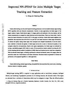
4 Simulation Results To evaluate the efficiency of the JPDAF algorithm, a 3-robot tracking scenario is considered. Fig.1 shows the initial position of the reference and target robots. To prepare the scenario and implement the simulations, the parameters are presented for the mobile robots structure and simulation environment as Table 2. Now, the following experiments are conducted to evaluate the performance of the JPDAF algorithm in various situations. Table 2 Simulation Parameters Parameters

Description

vl vr b ns Rmax Qs ts tmax

the robot’s left wheel speed the robot’s right wheel speed the distance between the robot’s wheels number of sensors placed on each robot the maximum range of simulation environment the covariance matrix of the sensors’ additive noise Sample time for simulation running Simulation maximum running time

Fig. 1 Initial Position of Reference and Target Robots and Simulation Environment, nonmaneuvering case

Multiple Target Tracking For Mobile Robots Using the JPDAF Algorithm

15

4.1 Local Tracking for Non-maneuvering Movement For each mobile robot, the speed of each wheel is determined as shown in Table 3. Table 3 Simulation Parameters Robot Number

Left Wheel Speed

Right wheel Speed

1 2 3

.2( Rad S ) .3( Rad S ) .1( Rad S )

.2( Rad S ) .3( Rad S ) .1( Rad S )

The initial position of the reference robot is set as [5, 5, Π2 ]. Also, the position of the target robots are considered as [8, 2, π ],[1, 3, Π3 ] and [1, 9, Π4 ], respectively. To run the simulation, sample time, ts , and simulation maximum running time, tmax , are set as 1s and 200s, respectively. Fig. 2 shows the trajectories generated for each mobile robot. To probe the physical environment, 24 sensors are placed on the reference robot. The sensors provide the distance from the static objects, walls or obstacles, and the dynamic targets. Because the position of each sensor to the robot’s head is fixed, the sensors’ data can be represented as a pair of [r, φ ] where φ is the angle between the sensor and the reference coordination. Also, the covariance of the sensors’ noise is supposed to be: µ

.2 0 0 5 × 10E − 4

¶ (32)

Now, the JPDAF framework is used to track the trajectory of each robot. In this simulation, the clutters are assumed to be the data collected from the obstacles such as walls. To apply the near constant velocity model as described in equation (27), the initial value of the velocity is chosen uniformly between 1 and -1 as follows: x˙t = U (−1, 1) y˙t = U (−1, 1)

(33) (34)

Where U (.) is the uniform distribution function. Fig. 3 presents the simulation results using the JPDAF algorithm with 500 particles for each robot’s tracking. Simulations justify the ability of the JPDAF algorithm in modifying the intrinsic error embedded in the data collected from the measurement sensor.

16

Aliakbar Gorji, Saeed Shiry and Mohammad Bagher Menhaj

4.2 Local Tracking for Maneuvering Movement Now, consider a maneuvering movement for each robot. Therefore, a variable velocity model is considered for each robot’s movement. Fig. 4 shows the generated trajectory for each mobile robot. Now, we apply the JPDAF algorithm for track-

Fig. 2 The generated trajectory for target robots

ing each robot’s position. To do so, 3 approaches are implemented. Near constant velocity model, near constant acceleration model and combined model described in the last section are used to estimate the states of the mobile robots. Fig. 5-7 shows the results for each robot separately. To compare the efficiency of each strategy, the obtained error is presented for each approach in Tables 4, 5 where the following criterion is used for estimating the error: t

ez =

max (zt − z˜t )2 ∑t=1 , zt = {xt , yt } tmax

(35)

The results show better performance of the combined method relative to the other approaches.

Multiple Target Tracking For Mobile Robots Using the JPDAF Algorithm

Fig. 3 The estimated trajectory using the JPDAF algorithm

Fig. 4 The generated trajectory for manoeuvering target robots

17

18

Aliakbar Gorji, Saeed Shiry and Mohammad Bagher Menhaj

Fig. 5 The estimated trajectory for robot 1

Fig. 6 The estimated trajectory for robot 2

Multiple Target Tracking For Mobile Robots Using the JPDAF Algorithm

19

Fig. 7 The estimated trajectory for robot 3 Table 4 The error for estimating xt Robot Number

Constant Acceleration

Constant Velocity

Combined

1 2 3

.0045 .0112 .0046

.0046 .0082 .0067

.0032 .005 .0032

Table 5 The error for estimating yt Robot Number

Constant Acceleration

Constant Velocity

Combined

1 2 3

.0082 .0096 .0073

.009 .0052 .0077

.0045 .005 .0042

5 Conclusion In this paper, the JPDAF algorithm was presented for multi robot tracking. After introducing the mathematical basis of the JPDAF algorithm, we showed how one can apply the JPDAF algorithm to the problem of multiple robot tracking. To do so, three different models were represented. The near constant velocity model and near constant acceleration model were first described and, then, combining two former approaches were presented as a modification to enhance the accuracy of multi robot tracking. Afterwards, simulation results were carried out in two different stages.

20

Aliakbar Gorji, Saeed Shiry and Mohammad Bagher Menhaj

First, tracking the non-maneuvering motion of the robots were explored. Later, the JPDAF algorithm was tested on tracking the motion of the robots with maneuvering movement. The simulations show that the combined approach provided better performance than the other presented strategies. Although the simulations were explored in the case in which the reference robot was assumed to be stationary, this algorithm can be easily extended to multi robot tracking as well as mobile reference robot. Indeed, robot’s self localization can be used to obtain the mobile robot’s position. Next, the JPDAF algorithm is easily applied to the target robots according to the current estimated position of the reference robot.

References 1. R. E. Kalman, and R. S. Bucy, New Results in Linear Filtering and Prediction, Trans. American Society of Mechanical Engineers, Series D, Journal of Basic Engineering, Vol. 83D, pp. 95– 108, 1961. 2. R. Siegwart and I. R. Nourbakhsh, Intoduction to Autonomous Mobile Robots, MIT Press, 2004. 3. A. Howard, Multi- robot Simultaneous Localization and Mapping using Particle Filters, Robotics: Science and Systems I, pp. 201–208, 2005. 4. N.J. Gordon, D.J. Salmond, and A.F.M. Smith, A Novel Approach to Nonlinear/non-Gaussian Bayesian State Estimation, IEE Proceedings F, 140(2):107–113, 1993. 5. M. Isard, and A. Blake, Contour Tracking by Stochastic Propagation of Conditional Density, In Proc. of the European Conference of Computer Vision, 1996. 6. D. Fox, S. Thrun, F. Dellaert, and W. Burgard, Particle Filters for Mobile Robot Localization, Sequential Monte Carlo Methods in Practice. Springer Verlag, New York, 2000. 7. C. Hue, J. P. L. Cadre, and P. Perez, Sequential Monte Carlo Methods for Multiple Target Tracking and Data Fusion, IEEE Transactions on Signal Processing, Vol. 50, NO. 2, February 2002. 8. B. Ristic, S. Arulampalam, and N. Gordon, Beyond the Kalman Filter, Artech House, 2004. 9. K. Kanazawa, D. Koller, and S.J. Russell, Stochastic Simulation Algorithms for Dynamic Probabilistic Networks, In Proc. of the 11th Annual Conference on Uncertainty in AI (UAI), Montreal, Canada, 1995. 10. F. Gustafsson, F. Gunnarsson, N. Bergman, U. Forssell, J. Jansson, R. Karlsson, and P. J. Nordlund, Particle Filters for Positioning, Navigation, and Tracking, IEEE Transactions on Signal Processing, Vol. 50, No. 2, February 2002 11. D. Schulz, W. Burgard, D. Fox, and A. B. Cremers, People Tracking with a Mobile Robot Using Sample-based Joint Probabilistic Data Association Filters, International Journal of Robotics Research (IJRR), 22(2), 2003. 12. M. S. Arulampalam, S. Maskell, N. Gordon, and T. Clapp, A Tutorial on Particle Filters for Online Nonlinear/Non-Gaussian Bayesian Tracking, IEEE Transactions on Signal Processing, Vol. 50, No. 2, February 2002. 13. N. Ikoma, N. Ichimura, T. Higuchi, and H. Maeda, Particle Filter Based Method for Maneuvering Target Tracking, IEEE International Workshop on Intelligent Signal Processing, Budapest, Hungary, May 24-25, pp.3–8, 2001. 14. R. R. Pitre, V. P. Jilkov, and X. R. Li, A comparative study of multiple-model algorithms for maneuvering target tracking, Proc. 2005 SPIE Conf. Signal Processing, Sensor Fusion, and Target Recognition XIV, Orlando, FL, March 2005. 15. T. E. Fortmann, Y. Bar-Shalom, and M. Scheffe, Sonar Tracking of Multiple Targets Using Joint Probabilistic Data Association, IEEE Journal of Oceanic Engineering, Vol. 8, pp. 173– 184, 1983.

Multiple Target Tracking For Mobile Robots Using the JPDAF Algorithm

21

16. J. Vermaak, S. J. Godsill, and P. Perez, Monte Carlo Filtering for Multi-Target Tracking and Data Association, IEEE Transactions on Aerospace and Electronic Systems, Vol. 41, No. 1, pp. 309–332, January 2005. 17. O. Frank, J. Nieto, J. Guivant, and S. Scheding, Multiple Target Tracking Using Sequential Monte Carlo Methods and Statistical Data Association, Proceedings of the 2003 IEEE/IRSJ, International Conference on Intelligent Robots and Systems, Las Vegas, Nevada, October 2003. 18. Jao. F. G. de Freitas, Bayesian Methods for Neural Networks, PhD thesis, Trinity College, University of Cambridge, 1999. 19. P. D. Moral, A. Doucet, and A. Jasra, Sequential Monte Carlo Samplers, J. R. Statist. Soc. B, 68, Part 3, pp. 411–436, 2006.