JCK(Wiley)
LEFT
INTERACTIVE
Multiple-Well, MultiplePath Unimolecular Reaction Systems. I. MultiWell Computer Program Suite JOHN R. BARKER Department of Atmospheric, Oceanic, and Space Sciences, Department of Chemistry, University of Michigan, Ann Arbor, MI 48109-2143 Received 5 July 2000; accepted 16 October 2000
ABSTRACT: Unimolecular reaction systems in which multiple isomers undergo simultaneous reactions via multiple decomposition reactions and multiple isomerization reactions are of fundamental interest in chemical kinetics. The computer program suite described here can be used to treat such coupled systems, including the effects of collisional energy transfer (weak collisions). The program suite consists of MultiWell, which solves the internal energy master equation for complex unimolecular reactions systems; DenSum, which calculates sums and densities of states by an exact-count method; MomInert, which calculates external principal moments of inertia and internal rotation reduced moments of inertia; and Thermo, which calculates equilibrium constants and other thermodynamics quantities. MultiWell utilizes a hybrid master equation approach, which performs like an energy-grained master equation at low energies and a continuum master equation in the vibrational quasicontinuum. An adaptation of Gillespie’s exact stochastic method is used for the solution. The codes are designed for ease of use. Details are presented of various methods for treating weak collisions with virtually any desired collision step-size distribution and for utilizing RRKM theory for specific unimolecular rate constants. 䉷 2001 John Wiley & Sons, Inc. Int J Chem Kinet 33: 232– 245, 2001
INTRODUCTION The purpose of this article is to describe the theoretical basis for the MultiWell computer program suite [1], which was designed for chemical kinetics calculations that involve complex coupled unimolecular reaction systems. Many chemical systems are characterized by the presence of multiple isomers that interconvert via unimolecular isomerization reactions while undergoing fragmentation reactions to form multiple sets of Correspondence to: J. R. Barker (
[email protected])
䉷 2001 John Wiley & Sons, Inc.
products. These systems are even more complex if excited species are produced via recombination reactions or chemical activation. In all of these cases, energy transfer involving weak collisions plays a role, and the resulting phenomenological reaction rates and branching ratios are functions of temperature, pressure, and the activation mechanism. MultiWell has been designed to simulate such systems. The MultiWell suite of computer programs includes MultiWell, which solves the master equation, and several tools. The tools consist of DenSum, which calculates sums and densities of states; Thermo, which
short standard long
JCK(Wiley)
RIGHT
INTERACTIVE
MULTIPLE-WELL, MULTIPLE-PATH UNIMOLECULAR REACTION SYSTEMS. I.
uses statistical mechanics formulas to calculate equilibrium constants and other thermodynamic quantities; and MomInert, which calculates principal moments of inertia and reduced moments of inertia for internal rotations. These computer programs are available from the author and from a Web site as free source code and makefiles for compiling on several platforms [1]. Example input and output files are available on the Web site. Note that the MultiWell package can be downloaded and examined in conjunction with this article. In the following article (Article II) [2], the MultiWell suite has been utilized to calculate reaction rates and product distributions for the 2-methylhexyl free radical isomerization/fragmentation system, which is comprised of six isomers connected via 15 reversible isomerization reactions [3]. Each isomer can decompose via C — C and C — H bond fission to produce a total of 14 distinct sets of fragmentation products [4]. In toto, there are 49 unimolecular reaction channels, all of which are treated specifically by using MultiWell. Examples are presented in Article II for chemical activation and shock-induced reactions. The results presented there illustrate some of the features incorporated in MultiWell. In this article, the theoretical basis for MultiWell is summarized. Inevitably, various approximations and assumptions must be adopted due to computational limitations and to the absence of physicochemical knowledge. The numerical approximations are described so that program users can better assess MultiWell’s limitations and strengths. The principal assumptions made in formulating the master equation are reviewed. In the next section, the master equation is described formally. In subsequent sections, the stochastic methodology is described along with a brief discussion of some of the merits and limitations of the hybrid master equation approach relative to other methods. Methods for computing microcanonical unimolecular reaction rates and energy transfer step sizes are described, followed by a description of various initial conditions that can be selected as options. Finally, the calculation input and output are outlined.
THE INTERNAL ENERGY MASTER EQUATION The current version of MultiWell is based on the onedimensional master equation, in which internal energy is modeled, but it is planned that future extensions will explicitly include angular momentum (the two-dimensional master equation [5 – 13]). The master equation
233
provides the fundamental theoretical basis for modeling systems in which both energy transfer and chemical reaction can occur [14 – 17]. It comprises a set of coupled integro-differential equations that describe the rates of production and loss of chemical species at specified energies.
Internal Energy and Active Degrees of Freedom Throughout this article, the internal energy E is assumed to be fully randomized among the active degrees of freedom. The internal energy for a particular species (stable molecule or transition state) includes the energy (measured from the zero-point energy) that resides in the internal modes (vibrations, torsions, and internal rotations) and an active external rotation. Nonlinear polyatomic species have three external rotational degrees of freedom characterized by moments of inertia IA , IB , and IC . The usual pragmatic approach [15] is to assume the molecule can be approximated as a symmetric top with two of the moments of inertia equal to one another (IA ⫽ IB), producing a degenerate two-dimensional external rotation. The third external rotor is associated with the symmetric top figure axis and is sometimes termed the K-rotor. The K-rotor is assumed to exchange energy freely with the other internal degrees of freedom, while the degenerate twodimensional external rotation is assumed to be inactive [14,15,17,18]. (More sophisticated treatments of rotations can be utilized in the present version of MultiWell by calculating specific rate constants (k(E)) externally and then providing them in data files read by MultiWell.)
Sums and Densities of States The MultiWell suite of computer codes includes DenSum, which utilizes the Stein-Rabinovitch [19] version of the Beyer-Swinehart algorithm [20] for exact counts of states for species comprised of separable degrees of freedom. The present version of DenSum can accommodate harmonic oscillators, Morse oscillators, and free rotors. The K-rotor is included with the internal degrees of freedom when calculating the sums and densities of states. There are two options for the treatment of rotations. The usual option is to use the convolution method developed by Astholz et al. [21], which is computationally efficient and accurate for rotors with small rotational constants. The second method is to use exact counts of rotational states. The second method is preferred if the rotational constant is larger than ⬃5 cm⫺1. DenSum produces an output file that is subsequently used as an input file by
short standard long
JCK(Wiley)
234
LEFT
INTERACTIVE
BARKER
MultiWell. The inactive two-dimensional external rotation is specified in the general MultiWell data file.
Master Equation for the Vibrational Quasicontinuum At high vibrational energies, a quasicontinuum of vibrational states exists and intramolecular vibrational redistribution (IVR) is rapid. Experiments show that IVR is slow at low energy, exhibits multiple time scales, and becomes rapid at energies where the vibrational state density is of the order of 102 – 103 states/ cm⫺1 [22]. At these state densities, some vibrational states overlap significantly within their natural widths as governed by infrared spontaneous emission rates. At state densities greater than ⬃107 states/cm⫺1, most states are overlapped within their natural widths. The onset of “rapid” IVR is a convenient marker for the onset of the vibrational quasicontinuum. However, this criterion leaves some uncertainty because IVR exhibits multiple time constants and thus some modes remain isolated even at higher vibrational state densities [22]. In the vibrational quasicontinuum, individual quantum states cannot be resolved and the master equation can be written: dy(E⬘,t) dE⬘ ⫽ f (E⬘,t)dE⬘ dt ⫹ ⫺ ⫺
冕 冕
⬁
dE[R(E⬘,E)dE⬘y(E,t)]
R(E,E⬘ )dE ⫽
dE[R(E,E⬘)dE⬘y(E⬘,t)]
0
R(E,E⬘ )dE
⬁
冎
(2a) (2b)
The second factor on the right-hand side of Eq. (2a), the integral over the rates of all inelastic transitions from initial energy E⬘, is the frequency of inelastic collisions, . Usually, the collision frequency is calculated from the expression ⫽ kcoll[M], where kcoll is the bimolecular rate constant for inelastic collisions (which in general may depend on E) and [M] is bath gas concentration. The first factor (in curly brackets) on the right-hand side of Eq. (2a) is P(E,E⬘ ) dE. It is important to emphasize that the factorization of R(E,E⬘ ) in Eq. (2) is merely for convenience and that kcoll and P(E,E⬘ ) never occur independently of one another. Furthermore, P(E,E⬘ ) is only a proper probability density function when is exactly equal to the inelastic collision rate constant. Under this assumption, P(E,E⬘ ) is normalized:
0
0
⬁
⫽ P(E,E⬘ )dE
⬁
⬁
冕 再
R(E,E⬘ )dE , 兰0 R(E,E⬘ )dE
冕
0
冘
vibrationally inelastic collision frequency () multiplied by the “collision step-size distribution,” P(E,E⬘ ), which expresses the probability that a molecule initially in the energy range from E⬘ to E⬘ ⫹ dE⬘ will undergo an inelastic transition to the energy range E to E ⫹ dE:
P(E,E⬘ )dE ⫽ 1
(3)
channels i ⫽ 1
k i (E⬘)y(E⬘,t)dE⬘
(1)
where y(E⬘,t)dE⬘ is the concentration of species with vibrational energy in the range E⬘ to E⬘ ⫹ dE⬘, R(E,E⬘ ) is the (pseudo-first-order) rate coefficient for VET from energy E⬘ to energy E, f(E⬘,t)dE⬘ is a source term (e.g., chemical or photoactivation), and ki(E⬘ ) is a unimolecular reaction rate constant for molecules at energy E⬘ reacting via the ith channel. Terms involving radiative emission and absorption have been omitted. In MultiWell, initial distributions are posited and the master equation is integrated to obtain time-dependent population distributions, reaction yields, and so on. Initial distributions appropriate for several common phenomena are discussed later. In the current version of MultiWell, the source term f(E⬘,t)dE⬘ on the right-hand side of Eq. (1) is not considered. If the rate coefficients R(E,E⬘ ) do not depend on the initial quantum states of the collider bath molecules, they can be written as the product of the total
Note that collision step-size distributions for activating and deactivating collisions are connected via detailed balance: P(E,E⬘ ) (E) ⫽ exp P(E⬘,E) (E⬘ )
再
⫺
E ⫺ E⬘ kBTtrans
冎
(4)
where (E) is the density of states at energy E, Ttrans is the translational temperature, and kB is the Boltzmann constant. The relationships among P(E,E⬘ ), kcoll, and the normalization integral are further discussed later.
Multiple Species (Wells) and Multiple Reaction Channels Here we consider chemical species that can be identified with local minima (wells) on the potential energy hypersurface. These species are distinct from transition states, which are located at saddle points. In MultiWell, each well is assigned an arbitrary index for
short standard long
JCK(Wiley)
RIGHT
INTERACTIVE
MULTIPLE-WELL, MULTIPLE-PATH UNIMOLECULAR REACTION SYSTEMS. I.
identification and reactions are conveniently labeled with two indices: one to designate the reactant and the other to designate the product. For simplicity in notation, one or more of these indices are omitted in some of the following discussion. A master equation such as Eq. (1) can be written for each well, and the equations are coupled via the chemical reaction terms. Each reaction channel is associated either with another well or with fragmentation products. Each isomerization is reversible, and the transition state is the same for the corresponding forward and reverse reactions. In principle, the existence of isomers leads to splitting of vibrational levels, as in the inversion doubling of ammonia, but if tunneling is negligible, the wells can be considered independently [23]. Thus, each well has its own vibrational assignment, molecular structure, and corresponding density of states. Two technical problems arise when using an energy-grained master equation [14,15,17,24] to simulate multiple-well systems. First, the number of coupled differential equations can grow prohibitively as the energy grain size (⌬Egrain) is reduced, making the numerical solution very difficult or impossible. Second, because each well has its own zero of energy and reaction threshold (critical) energies, it is difficult to match the energy-grain boundaries. The reaction threshold energies for forward and reverse reactions are tied to one another. For accurate numerical results, it is necessary to match the energy grains of the coupled wells. The matching of energy grains at one reaction threshold may lead to mismatches at other thresholds and to artificially shifted energies of the wells, relative to one another. These energy shifts produce anomalous results for large grain sizes. This problem can be neglected if the energy grains are very small, but small energy grains lead to very large sets of coupled equations. In all cases, the calculations should be repeated with successively smaller energy grains until the results are independent of ⌬Egrain: Convergence must be achieved. When a continuum master equation is used, energy mismatching and anomalous shifts never create problems. However, the sparse density of states regime at low energies within wells and for transition states near reaction thresholds is not well represented by a continuum model. This difficulty is minimized in MultiWell by using a hybrid master equation approach.
Hybrid Master Equation Formulation Effectively, this formulation uses a continuum master equation in the quasicontinuum at high vibrational energies and an energy-grained master equation at low
235
energies, where the state density is distinctly discontinuous. This is accomplished by using Eq. (1) for the continuum master equation throughout the entire energy range but discretizing the state density, population, and transition rates at low energy. At high energy, Multiwell employs interpolation to determine the density of states and specific rate constants (k(E)). Values of (E) and k(E) are stored in ordered arrays at specific values of E, and intermediate values are determined by interpolation. At low energies, ordered arrays of (E) and k(E) are stored at smaller energy spacing (⌬Egrain) and interpolation is not used: The array entries nearest in energy are utilized directly. The two ordered arrays used for each energy-dependent quantity ((E), k(E), etc.) are combined in “double arrays,” which are discussed in the next section. At all energies, numerical integration is carried out with the trapezoidal rule, which introduces an energy grain in the low energy regime (where state densities are sparse) but gives good continuum results at high energy (where the state densities are smooth). If a stochastic trial (see later) calls for a transition from the continuum space to an energy in the discrete space, the energy is aligned with the discrete energy grain. At low energy, many energy grains do not contain states ((E) ⫽ 0) and transitions are not allowed to those states in MultiWell. As a result, population only resides in energy grains that contain states and collisional transitions low on the energy ladder can only take place with relatively large energy changes, due to the sparse density of states.
Energy Grain in the Hybrid Master Equation Through the use of double arrays, high-energy resolution is achieved in densities and sums of states at low energy and near reaction thresholds. By default, the double arrays have 500 elements (the dimensions can be changed, if desired). The low energy portion of the array is specified according to ⌬Egrain and the number of array elements assigned to the low energy portion of the double array. The high-energy portion is specified only according to the maximum energy. Thus, the number of array elements used in the highenergy portion and the energy grain in the high-energy portion both depend on how many array elements remain after assigning the low energy portion. The same specifications are used for all double arrays, including arrays for densities of states ((E)), sums of states (G‡(E ⫺ E0)), specific rate constants (k(E ⫺ E0)), etc. The discretization of these quantities is the natural result of exact-count algorithms. An example of a double array for the density of states (E) is shown in Figure 1 for benzene (vibra-
short standard long
JCK(Wiley)
236
LEFT
INTERACTIVE
BARKER
Figure 1 Density of states for benzene (including vibrations and one active external rotation). Solid line: density of states from exact count (⌬Egrain ⫽ 10 cm⫺1); solid dots: elements of double array (see text for details).
Typical convergence tests [2] show that 250 bins with ⌬Egrain ⫽ 10 cm⫺1 are usually suitable for the low energy portion of the double arrays. The upper energy bound for the high energy portion is typically 85,000 cm⫺1 to 100,000 cm⫺1, depending on the temperature range and activation method being simulated. The small grain at every reaction threshold gives accurate results for the unimolecular reaction rates. The small grain at low energy within each well gives a good representation of the sparse density of states regime in every well. To achieve comparable numerical results by the matrix solution [17] of an energy-grained master equation for just a single well would require finding the eigenvalues of a matrix with 8500 ⫻8500 elements — a difficult task. The hybrid master equation approach has a distinct advantage in this regard.
STOCHASTIC METHOD tions [25] ⫹ K-rotor). In this example, the density of states was calculated using an energy grain of ⌬Egrain ⫽ 10 cm⫺1 and exact counts up to an energy of 85,000 cm⫺1, although only energies up to 10,000 cm⫺1 are shown in the figure. In this example, the low energy regime was defined as the first 250 elements of a double array and thus covered the range from 0 to 2490 cm⫺1. The remaining 250 elements of the double array overlap the low energy portion and cover the range all the way from 0 to 85,000 cm⫺1 (the high energy regime) with an energy grain of 341.4 cm⫺1. In Figure 1, (E) calculated with ⌬Egrain ⫽ 10 cm⫺1 is shown as the thin solid line and the double array elements are shown as the solid dots. The upper energy boundary for the low energy range was chosen to fall within the vibrational quasicontinuum, as evidenced by (E) ⱖ 100 states/cm⫺1 and by the relative smoothness of the plot of (E). When (E) is sufficiently smooth, relatively little error is introduced by interpolating between the double array points. In principle, convergence tests should be carried out for each simulation. Tests for convergence as ⌬Egrain is reduced reflect several simultaneous effects: The (E) grain size is varied for every well, the G‡(E ⫺ E0) grain size is varied for every reaction, and the energy range covered by the low energy portion of every double array is varied. Because several attributes are affected by ⌬Egrain, the variation of results with grain size cannot be interpreted precisely without extensive tests. However, as long as the energy range covered by the low energy portion of the double arrays is sufficient, smaller grain sizes will produce more accurate results and the results are seen to converge at small ⌬Egrain, as illustrated in Figure 4 of Article II [2].
Gillespie’s Exact Stochastic Method Gillespie showed that a stochastic method gives the exact solution to a set of ordinary differential equations in the limit of an infinite number of stochastic trials [26,27]. The algorithm has been described in the context of chemical kinetics [28,16]. If a Markovian system is in a given state and can make transitions to other states via a set of transition rate coefficients, then for a given step in a stochastic simulation, Gillespie’s algorithm gives a prescription for (a) finding the duration of the time step and (b) selecting the transition from among the choices. This algorithm is repeated step-by-step as long as desired and as long as transitions are possible. Gillespie’s method can be applied to both linear and nonlinear systems [28]. Equation (1) is linear in y(E,t), which leads to a particularly convenient result that is described later. If Eq. (1) contained nonlinear terms to describe energy pooling; for example, the terms would contain factors such as the product y(E,t) ⫻ y(E⬘,t). To solve this system numerically requires using an energy-grained master equation with a swarm of stochastic trials and storing an evolving vector of populations as a function of energy. Here, the number of stochastic trials can be identified with a number of pseudomolecules that initially are placed in a set of energy grains. At each time step, a pseudomolecule is moved from one energy grain to another, as described by Gillespie, and the swarm of pseudomolecules maps out the evolving energy distribution. This approach has been used by Veerecken et al. [29] to simulate unimolecular and recombination reactions, and it can in principle be extended to non-
short standard long
JCK(Wiley)
RIGHT
INTERACTIVE
MULTIPLE-WELL, MULTIPLE-PATH UNIMOLECULAR REACTION SYSTEMS. I.
linear systems. The difficulties in this approach are associated with the energy-grained master equation (see earlier) and with the requirement for storage of the entire vector of y(E,t) at every time step. Given the current availability of inexpensive computer memory, the latter is not a serious limitation for single-well reaction systems. When several wells are involved, the bookkeeping is cumbersome. Moreover, the memory requirements of this technique can become prohibitive in the future if the one-dimensional master equation is to be extended to two dimensions by explicitly including angular momentum. MultiWell is designed so that the future extension to two dimensions will be feasible. For linear master equations, a different strategy [16] is possible using Gillespie’s algorithm. Instead of using a swarm of stochastic molecules and storage of y(E,t) at every step, stochastic trials are run one at a time and snapshots of E and other variables are stored at convenient time intervals. The vector y(E,t) does not need to be stored. A “snapshot” simply records the energy and other properties of a single stochastic molecule as it progresses through a stochastic trial. The snapshot has no effect on the physics of the trial. Since the system is linear, the averaged result of an ensemble of stochastic trials gives the same result as a swarm of stochastic molecules. By retaining only the averaged results of the snapshots, the memory storage requirements are greatly reduced. For a linear master equation, the loss terms can be expressed as first-order in y(E,t) with first-order rate coefficients Aj for k paths. These rate coefficients can be identified with the unimolecular rate constants and the collision frequency in Eq. (1). According to Gillespie’s algorithm, the duration of the next time step is chosen by using the uniform random deviate (i.e., random number) r1:
⫽
⫺ln(r1 ) AT
(5a)
冘A
(5b)
where AT ⫽
k
j⫽1
j
The transition is selected from among the k paths by using a second random number, r2:
冘A ⬍rA ⱕ冘A
n⫺1 j⫽1
k
j
2
T
j⫽n
j
(6)
Here, the transition takes place via path n at time t ⫹ .
237
According to Gillespie’s algorithm, the time intervals between stochastic steps are chosen randomly by Eq. (5a). Thus, the progress of the stochastic simulation is monitored via snapshots, as mentioned earlier. If collisional activation or deactivation is the result of a transition, then the next stochastic step is calculated using rate coefficients appropriate to the new energy. If isomerization to another well is the result of a transition, then the next stochastic step is calculated using the first-order rate coefficients appropriate to the new well, based on E measured from the zero-point energy of the new well. The snapshots from many stochastic trials are averaged. The results include the time-dependent average fractional populations of the isomers, the average internal energy of each isomer, and fractional yields of the fragmentation products, etc. The computer time required for any given stochastic simulation depends on Ntrials, the simulated time duration, and on the properties of the system that affect AT in Eq. (5b). For example, one of the Aj terms is the collision frequency, which is proportional to pressure. If the collision frequency is the dominant term in Eq. (5b), then the average stochastic time step is inversely proportional to pressure, and the number of time steps (and the corresponding computer execution time) for the given simulated time duration is proportional to pressure. Of course, collision frequency is not always the dominant term in Eq. (5b), but the same qualitative considerations can help in estimating required computer time. Note that the effectiveness of Eq. (6) is limited by the properties of the random number generator. The characteristics of various random number generators are discussed elsewhere [30 – 32], where many potential pitfalls are described. It is important to use random number generators that have been thoroughly tested. Even assuming the random number generator produces a sequence that has no serial correlations, the number of random numbers in a sequence is limited, and this imposes a limitation on the relative magnitudes of the Am terms that can be selected according to Eq. (6). For a 32-bit computer, a typical random number sequence contains 231 ⫺ 1 ⬇ 2.1 ⫻ 109 equally spaced numbers. Thus, if the ratio of minimum to maximum values of the rate constants is less than ⬃0.5 ⫻ 10⫺9, then the path with the smaller rate can never be selected. Thus, the random number generator places a rigorous upper bound on the dynamic range of rates that can be selected. A more serious limitation, however, is that an extraordinarily large number of stochastic trials is required in order to sample rare events with useful precision, as discussed in the next section.
short standard long
JCK(Wiley)
238
LEFT
INTERACTIVE
BARKER
Stochastic Uncertainties The precision of the results obtained using stochastic methods depends on the number of stochastic trials. In the systems simulated by MultiWell, several species coexist and their relative populations sum to unity: 1 ⫽ f1 ⫹ f2 ⫹ · · · ⫽
冘
species i⫽1
fi
(7)
The standard deviation in the instantaneous relative population of the ith species is the square root of the variance calculated according to the multinomial distribution [33]:
i ⫽
q
1 fi(1 ⫺ fi ) Ntrials
(8)
where fi is the fractional population of the ith species and Ntrials is the number of stochastic trials. Note that the standard deviation is reduced as the number of trials increases. Also note that fi and (1 ⫺ fi) appear symmetrically in Eq. (8). Thus, the standard deviation is the same when, for example, fi ⫽ 0.01 and when fi ⫽ 0.99. These standard deviations are calculated and reported by MultiWell in its general output. A large number of stochastic trials is needed when rare events must be simulated with high precision. Suppose that fi ⫽ 0.01 and the desired precision corresponds to a relative statistical error of 1% (i.e., i /fi ⫽ 0.01). From Eq. (8), one finds the required number of stochastic trials: Ntrials ⬇106. For a relative error of 10%, only about 104 trials are needed. Thus, the required number of stochastic trials places a practical limit on the precision attainable for minor pathways.
PROCESSES Unimolecular Reactions The energy-dependent specific unimolecular rate constant k(E) is given by the RRKM statistical theory [14,15,17,18]: k(E) ⫽
冋
m‡ ext m ‡ext
册
g‡e 1 G ‡(E ⫺ E0 ) ge h (E)
(9)
where m‡ and m are the number of optical isomers [17]; ext‡ and ext are the external rotation symmetry numbers; ge‡ and ge are the electronic state degeneracies of the transition state and reactant, respectively; h is Planck’s constant, G‡(E ⫺E0) is the sum of states of the transition state; E0 is the reaction threshold en-
ergy; and (E) is the density of states of the reactant molecule. The internal energy E is measured relative to the zero-point energy of the reactant molecule, and the reaction threshold energy (critical energy) is the difference between the zero-point energies of reactant and transition state. Equation (9) was written by assuming that the rotational external symmetry numbers were not used in calculating the sums and densities of states [17]. It is, however, assumed that internal rotor symmetry numbers are used explicitly in the sum and density calculations and hence do not appear in Eq. (9). Note that the quantity set off in square brackets is the reaction path degeneracy [17]. For a tight transition state, G‡(E ⫺ E0) can be calculated from a vibrational-rotational assignment, and the reaction threshold energy can be corrected approximately for angular momentum effects by using a pseudodiatomic model [15,17]. According to this approximation in thermal systems, the temperature-corrected threshold energy E0T is given by the following expression: E0T ⫽ E0 ⫺ kBTtrans
再
1⫺
IA I ‡A
冎
(10)
where IA and I ‡A are the moments of inertia for the external two-dimensional inactive rotations of the reactant and of the transition state, respectively. For loose transition states, more elaborate techniques are needed for calculating k(E). Such techniques include Variational Transition State Theory [17,18], Adiabatic Channel Model [34], and Flexible Transition State Theory [35]. Computer codes have been published for some of these theories [36,37]. These methods can be used in the current version of MultiWell by calculating k(E ⫺ E0) externally and then reading the values from a data file. MultiWell will accept double arrays (from external files) that specify G‡(E ⫺ E0) (which can be calculated conveniently using codes like DenSum, part of the MultiWell suite) or that specify k(E ⫺ E0). Since a double array is used, the effective energy grain can be very small near the reaction threshold, where high energy resolution is important. Another selectable option in MultiWell is to calculate k(E) using the inverse Laplace transform method described by Forst [15,38]: k(E) ⫽
冋
m‡ ext m ‡ext
册
g‡e (E ⫺ E⬁ ) A ge ⬁ (E)
(11)
where A⬁ and E⬁ are the Arrhenius parameters for the corresponding high-pressure-limiting thermal rate constant. Note that the reaction path degeneracy (the
short standard long
JCK(Wiley)
RIGHT
INTERACTIVE
MULTIPLE-WELL, MULTIPLE-PATH UNIMOLECULAR REACTION SYSTEMS. I.
quantity in square brackets) can be absorbed into A⬁ if desired. For added accuracy near the reaction threshold, E⬁ may be replaced in Eq. (11) by Eo, the threshold energy. This substitution may improve the threshold behavior, but it introduces a small error in the calculated high-pressure-limit activation energy. Regardless of the method for calculating k(E), the unimolecular rate constant at the high pressure limit, k⬁(Ttrans), is calculated in MultiWell by using (E) and k(E): k⬁ (Ttrans ) ⫽ 1 Q(Ttrans )
冕
⬁
E0
k(E) (E)exp(⫺E/kBTtrans )dE
(12)
where Q(Ttrans) is the partition function of the reactant internal degrees of freedom (the degrees of freedom used to calculate (E) and k(E)) at translational temperature Ttrans: Q(Ttrans ) ⫽
冕
⬁
0
(E)exp(⫺E/kBTtrans )dE
(13)
The numerical integrations are carried out using the trapezoidal rule, because (E) fluctuates wildly at low energies. Tests show that the numerical integration produces values for k⬁(Ttrans) that are accurate within a fraction of 1% for usual values of ⌬Egrain [2]. The activation energy is obtained by calculating k⬁(Ttrans) at two closely spaced temperatures: E⬁ ⫽ ⫺ R
ln[k⬁ (T2)/k⬁(T1)] [T2⫺1 ⫺ T1⫺1 ]
(14)
From the activation energy and the rate constant at one temperature, the A-factor (A⬁) can be calculated. Values for k⬁(Ttrans), E⬁, and A⬁ calculated in this way are reported (for each reaction) in the general output file.
Collisions Frequency of Inelastic Collisions. Conventionally, it is assumed that the inelastic collision frequency is the same as that experienced by molecules subject to a Lennard-Jones intermolecular potential. For the Lennard-Jones potential, kcoll takes the following form [24]: kcoll ⫽ 2具 典 ⍀ (2,2)*
(15)
where 具 典 is the average speed at the translational temperature, is the Lennard-Jones diameter, and
239
⍀(2,2)* is the collision integral [39], which depends on the Lennard-Jones parameters. Since only the product kcollP(E,E⬘ ) appears in the master equation, if kcoll is underestimated, then normalization of the step-size distribution is not appropriate. If, on the other hand, kcoll is overestimated, then P(E,E⬘ ) must include elastic collisions [40]. The inclusion of elastic collisions in the master equation causes no problems, except to reduce the efficiency of certain numerical solutions. However, the fundamental question remains: Is the frequency of inelastic collisions the same as the Lennard-Jones collision frequency? Lawrance and Knight [41] used single vibrational level fluorescence and found that the observed total cross sections for inelastic collisions are in quantitative agreement with the Lennard-Jones collision frequency for a moderately high density of vibrational states. Classical trajectory calculations support this assumption [42,43], but the argument is somewhat circular in this case since the assumed potential energy functions are often constructed from pairwise Lennard-Jones potentials. Very recently, Xue et al. [44] used quantum beat spectroscopy to investigate a single vibrational level of SO2 at high vibrational energy and found cross sections substantially greater than predicted by the Lennard-Jones interaction potential. However, in the sparse density of states regime at low vibrational energies it is well known that the inelastic collision cross section is small [45], and thus the total inelastic collision rate constant is probably smaller than kLJ . A rigorous upper limit to kcoll is provided by the total collision rate constant kq , which is based on the total quantum cross section. Because of concern about the proper choice of kcoll and normalization of the stepsize distribution (see later), MultiWell provides an option for utilizing the total collision rate constant, which can be estimated from Lennard-Jones parameters [46]. Since it is expected that the fraction of inelastic collisions is small at low energy (see earlier) and cannot exceed unity at high energies, the following heuristic function has been included as an option in MultiWell: kcoll ⫽ kq{1 ⫺ exp[⫺(E ⫺ Eq )/b]}
(16)
where Eq and b are empirical parameters that regulate the energy dependence of kcoll. This option has been made available in MultiWell, but it has not yet been investigated thoroughly. Collision Step-Size Distribution. Many step-size distribution models have been used in energy transfer studies, and there is still considerable uncertainty about the appropriate collision model and functional
short standard long
JCK(Wiley)
240
LEFT
INTERACTIVE
BARKER
form of P(E,E⬘ ) [47,48]. Note that Pd(E,E⬘ ) for deactivating collisions is expressed in terms of an unnormalized function, fd(E,E⬘ ), and normalization factor N(E): 1 fd(E,E⬘ ), N(E⬘ )
Pd(E,E⬘ ) ⫽
for E⬘ ⬎ E
(17)
To offer a wide selection, MultiWell includes ten different optional functional forms for fd(E,E⬘ ), including biexponential, Gaussian, Weibull distribution, etc. The best information currently available suggests that a generalized exponential function is most appropriate for deactivation steps [48,49]: fd(E,E⬘ )
再
冨
⫽ exp ⫺
E⬘ ⫺ E ␣(E⬘ )
冨 冎, ␥
for E⬘ ⬎ E
(18)
where ␣(E) is a linear function of vibrational energy and ␥ is a parameter that ranges from ⬃0.5 to ⬃1.5. The corresponding expression for activation collisions is obtained from detailed balance Eq. (4). When the parameter ␥ is less than unity, the wings of the stepsize distribution have enhanced relative probabilities that qualitatively resemble the biexponential distribution. When ␥ ⫽ 1, Eq. (18) gives the venerable exponential model. Normalization. When kcoll is the exact rate constant for inelastic collisions, the step-size distribution function is normalized:
冕
⬁
0
P(E,E⬘ )dE ⫽ 1
(19)
The normalization factor can be partitioned into separate terms for activating (Na(E)) and deactivating (Nd(E)) collisions: N(E) ⫽
冕
E
0
⫹
fluctuations and some energy grains may contain no states, while the function is quite smooth at high energies. Since it is desirable to be able to use arbitrary functions for the collision step-size distribution, it is not feasible to employ analytic expressions for the integrals in Eq. (20), which would allow much shorter computer execution times. In fact, several approximate analytical expressions were tested, but none was sufficiently accurate in the sparse density of states regime. For this reason, normalization is carried out numerically using the open-ended trapezoidal rule, which is a particularly robust algorithm [32]. For low energies, the energy step size is set equal to that used in the lower energy portion of the double arrays (⌬Egrain). At higher energies, the energy step size is set equal to a fraction (typically 0.2) of the magnitude of a characteristic energy transfer step:
␦Ed ⫽
冨d(ln f dE(E, E⬘))冨
, for E⬘ ⬎ E,
(21a)
␦Ea ⫽
冨
, for E⬘ ⬍ E,
(21b)
⬁
E
fa (E,E⬘ )dE ⫽ Nd (E) ⫹ Na(E)
d(ln fa (E⬘, E)) dE
冨
⫺1
where fa(E,E⬘ ) and fd(E,E⬘ ) were defined earlier. For the exponential model, ␦Ed is equal to ␣(E), which varies with internal energy. In general, both the characteristic energy length and the integration step size vary with energy. Monte Carlo Selection of Step Size. Two random numbers are used for selecting the collision step size. The first random number selects activating, or deactivating, collisions by comparison to the up-transition probability, Pup(E): Pup(E) ⫽ Na(E)/N(E),
fd (E,E⬘ )dE
冕
⫺1
d
up-transition probability (22)
0 ⱕ r3 ⬍ Pup(E), Pup(E) ⱕ r3 ⬍ 1,
(20)
where fd(E,E’) was defined earlier. The unnormalized function for activating collisions, (fa(E,E’)), is calculated with the aid of the detailed balance expression Eq. (4). For convenience in the Monte Carlo selection of step sizes, both the normalization factor, N(E), and the probability of an activating collision, [Na(E)/N(E)], are stored in double arrays for each well. At low state densities, P(E,E⬘) exhibits random
activating
(23a)
deactivating
(23b)
To select the step size, the second random number is used with the cumulative distribution for P(E,E⬘ ) to find the final energy E, given initial energy E⬘ [16]: r4 ⫽
冕 冕
E
1 Na(E⬘)
1 r4 ⫽ Nd(E⬘)
E⬘
fa(x, E⬘)dx,
activating
(24a)
E
E⬘
fd(x, E⬘)dx,
deactivating
(24b)
short standard long
JCK(Wiley)
RIGHT
INTERACTIVE
MULTIPLE-WELL, MULTIPLE-PATH UNIMOLECULAR REACTION SYSTEMS. I.
The integrals are evaluated by the trapezoidal rule, just as described in the preceding section, until the equalities in Eq. (24) are satisfied. In the high energy regime, this is accomplished by integrating step-bystep until an integration step gives a value for the righthand side of Eq. (24) that is larger than r4. Linear interpolation is then used to find the value of final energy E that satisfies the equality. In the low energy regime, the integration is carried out step-by-step to find the energy step that gives the best agreement between the LHS and right-hand side of Eq. (24). Note that the normalization integrals in the low energy regime are stored in the lower energy portion of the double arrays. In the high-energy regime, the normalization integrals are found by interpolation of values stored in the high-energy portion of the double arrays. Occasionally, the normalization integrals are overestimated due to imperfect interpolation, and thus the equalities in Eq. (24) cannot be satisfied. In such a case, the integral is evaluated step-by-step until the additional partial sum is less than a selected relative error (typically 10⫺6). This procedure yields an explicitly calculated value for the normalization integral. The interpolated normalization integral is then replaced with this new value, and the energy step selection process is repeated. This procedure is somewhat cumbersome and computationally intensive, but it was found to produce numerically accurate thermal distribution functions.
Other Processes Additional processes can be incorporated into MultiWell calculations by using the capability of reading rate constants from external data files. For example, Moriarity and Frenklach [50] have used MultiWell for assessing several complicated reaction paths that may lead to aromatic ring formation in combustion systems. They found that certain vibrationally excited intermediates persist for relatively long periods and therefore bimolecular reactions between energized adducts and gaseous partners may need to be included in future calculations. In fact, such processes can be included in MultiWell, if the gaseous partner is in excess, so that the pseudo-first-order approximation can be invoked and a pseudo-first-order rate constant (kI) can be defined. The pseudo-first-order rate constant kI can be introduced as an irreversible unimolecular reaction and read from a data file. This is particularly simple to implement if it can be assumed that kI is independent of vibrational energy. The vibrational energy dependence of the bimolecular reaction rate constant in principle can be included by using microcanonical transition state theory [51 – 54]. Several processes have been neglected in the
241
present version of MultiWell. For example, spontaneous infrared emission [55] by the vibrationally excited species, which is particularly important at low pressure [56], has not been included. Similarly, stimulated emission, which is important in laser-induced chemical reactions [57,58], has also been neglected. Future versions of MultiWell may include these processes, especially if the kinetics community expresses an interest in them.
INITIAL CONDITIONS At the start of each stochastic trial, initial conditions must be specified. MultiWell selects the initial energy via Monte Carlo selection techniques that are based on the cumulative distribution function corresponding to a selected physical process. It is assumed that the reactant is at infinite dilution in a heat bath and thus there are no temperature changes due to reaction exothermicity or energy transfer. For most laboratory experiments, this is an acceptable approximation.
Monte Carlo Selection of Initial Energies Monte Carlo selection of the initial internal energy is carried out by equating random number r5 to the cumulative distribution function Y0(E) corresponding to a given initial energy density distribution y0(E⬘ ): r5 ⫽ Y0(E) ⫽
冕
E
0
y0 (E⬘)dE⬘
(25)
where E⬘ is the integration variable. In MultiWell, Y0(E) is found by trapezoidal integration, and the values are stored as a function of initial energy in a linear array. For the default array dimensions, 500 array elements are used to cover the relevant energy range. For a thermal distribution (see later), the relevant energy range is assumed to be ⬃20kBT. The Monte Carlo selection is carried out by interpolating in the stored array to find the value of E at which Y0(E) ⫽ r5. Interpolation in this fashion is much more computationally efficient than calculating the integral in Eq. (25) for each stochastic trial.
Optional Initial Energy Density Distributions The initial energy density distributions that are included as options in MultiWell are described here. In addition to these choices, there is also a provision for providing a user-defined double array of Y0(E) values and for a delta function (which does not require Monte
short standard long
JCK(Wiley)
242
LEFT
INTERACTIVE
BARKER
Carlo selection). Examples of user-defined functions include prior distributions [29,59] and energy distributions that are the result of bond fission [60].
y(ca,i) (E)dE 0 ⫽
冕
ki(E)(E)exp(⫺E/kBTvib) dE
⬁
E0
Thermal Activation. In an ordinary thermal unimolecular reaction system that takes place at infinite dilution, the translational and vibrational temperatures are equal and do not change during reaction (Ttrans ⫽ Tvib). For shock wave simulations, it is assumed that Ttrans changed instantaneously when the shock occurred and therefore is elevated at t ⫽ 0 but Tvib remains at the temperature that described the thermal system prior to the shock. Subsequent vibrational energy transfer collisions cause the internal energy to increase. The only difference between shock tube and isothermal simulations is that in the former, the two temperatures are unequal. In both cases, the initial internal energy distribution function is a Boltzmann distribution characterized by Tvib. The probability of the initial energy E falling in the range between E and E ⫹ dE is given by the probability density function y(therm) (E)dE ⫽ 0
冕
(E)exp(⫺E/kBTvib) dE
⬁
0
(26)
(E⬘)exp(⫺E⬘/kBTvib) dE⬘
Single Photon Photoactivation. The energy distribution produced by absorption of a single photon is assumed to be described by the thermal population at the ambient vibrational temperature added to the energy of the photon (h). Hence, the probability density function for photoactivation is given by Eq. (26), and the selected thermal energy is then increased by h. Chemical Activation and Recombination Reactions. Chemical activation is the process by which a single vibrationally excited species (C) is produced from the bimolecular reaction of two precursor species (A and B): A ⫹ B : C(E)
(27)
where E is the vibrational energy. The chemical activation distribution function is obtained from the reverse reaction by using detailed balance [14,15,17,24]. The reverse reaction is the unimolecular decomposition reaction with rate constant ki(E) that produces the product set A ⫹ B. The index i specifies the particular unimolecular reaction channel. The resulting density function is a thermal distribution weighted by ki(E). The probability density function and corresponding Monte Carlo selection expression are as follows:
,
ki(E⬘)(E⬘)exp(⫺E⬘/kBTvib) dE⬘ for E ⱖ E0 r5 ⫽
冕
(28)
E⬘
E0
y (ca,i) (E)dE 0
(29)
where the lower limits in Eqs. (28) and (29) are equal to E0, the unimolecular reaction threshold energy. The trapezoidal rule is used in the selection procedure, as described earlier for thermal activation. A recombination reaction produces a recombination product, which is a chemically activated species. The chemically activated recombination product C(E) can react via the reverse of reaction (27), and possibly by other unimolecular pathways, in competition with collisional energy transfer. Several quantities may be of interest, including branching ratios, net rates of reaction to produce specific final products, and so on. In all cases, the first step is to simulate the reactions of the chemically activated recombination product C(E) under the desired conditions of temperature and pressure. The results of the simulation can be used in various ways to find the quantities of interest (see Article II). The total rate constant for the recombination reaction at the high-pressure limit is obtained from detailed balance by using the equilibrium constant K(Ttrans) at translational temperature Ttrans: krec,⬁ ⫽ kuni,⬁/K(Ttrans)
(30)
where krec,⬁ and kuni,⬁ are the high-pressure-limiting recombination and unimolecular decomposition rate constants, respectively; the latter of these is calculated and reported in the MultiWell standard output. The equilibrium constant K(Ttrans) is calculated using the program Thermo (part of the MultiWell computer program suite), which employs standard statistical mechanics formulas [61,62] for the partition functions of the reactants A and B. For the partition function of C, Thermo utilizes Eq. (13) and the same densities of states employed by MultiWell to calculate the partition function given by Eq. (13). To calculate the overall rate constant for producing the ith product, the relative population (fraction) fi of that species at the end of the simulation is multiplied by krec,⬁: k ⫽ fikrec,⬁ ⫽ fikuni,⬁/K(Ttrans)
(31)
short standard long
JCK(Wiley)
RIGHT
INTERACTIVE
MULTIPLE-WELL, MULTIPLE-PATH UNIMOLECULAR REACTION SYSTEMS. I.
INPUT Major Options Densities of States: (E). Densities of states for the wells can be provided in either of two ways. They can be calculated internally according to the Whitten-Rabinovitch approximation [63,64], or they can be provided in an external file (in the form of a double array). The second approach is preferred, because the sums and densities can be calculated externally by an exactcount algorithm, which is much more accurate than the Whitten-Rabinovitch approximation. DenSum is provided as a tool to calculate sums and densities of states according to the Whitten-Rabinovitch approximation or according to the Stein-Rabinovitch method [19] of exact counts. Molecular assignments for use in the current version of DenSum can be expressed in any combination of separable harmonic oscillators, Morse oscillators, and free rotors. For nonseparable degrees of freedom, other approaches will be needed (see [65] for an example). The moments of inertia needed for calculating rotational constants are evaluated with the program MomInert. This code requires Cartesian coordinates for the molecular structure. Such structures can be calculated with good accuracy by using quantum chemistry programs. Specific Unimolecular Rate Constants: k(E). Specific rate constants are needed for each reaction. There are three ways to provide rate constants: (a) They may be calculated internally via the inverse Laplace transform method, (b) the sums of states can be provided in an external file, and (c) the k(E) values can be provided in an external file. Data provided in an external file is in the form of a double array with energy origin at the reaction threshold energy. The double array allows high energy resolution near the reaction threshold where it is most important. For most purposes, it is most efficient to use DenSum, which calculates sums of states (G‡(E ⫺ E0)) and generates an external file suitable for input into MultiWell. However, Densum is only suitable for fixed transition states with separable degrees of freedom and therefore other methods must be used to calculate G‡(E ⫺ E0) or k(E ⫺ E0) for nonseparable and flexible transition states. If the reaction is a reversible isomerization reaction, MultiWell uses the same external data file to calculate k(E ⫺ E0) for both forward and reverse reactions. By using the same external file for both forward and reverse reactions, the reversible isomerization rates are internally self-consistent.
243
Properties of Wells and Transition States Energies (e.g., ⌬Hf⬚ at 0 K) are required for all wells and transition states in order to establish the relative energies of isomers and reaction thresholds. Moments of inertia are needed for the inactive degenerate twodimensional external rotation. Energy transfer parameters are needed for each well, and MultiWell does not require that they be the same for all wells. One would expect the energy transfer parameters for a cyclic species to differ from those of a linear isomer. However, to the best of my knowledge the energy transfer parameters are not known for more than one isomer in any system. Until additional information becomes available, it is pragmatic to assume that all isomers have the same energy transfer parameters.
OUTPUT MultiWell generates several output files that summarize the input data and the calculation results. MultiWell.OUT: This general output file summarizes the input parameters, thermochemistry, highpressure-limit rate constants for each reaction, time-dependent average fractional populations (with standard deviations from Eq. (11)), and average vibrational energies. The time-dependent quantities are the instantaneous (snapshot) values averaged over Ntrials stochastic trials; they are not averaged over the time interval, as was done in previous master equation codes from this laboratory [16,66,67]. MultiWell.RATE: This file stores the time-dependent output of average unimolecular rate “constants” (which vary with time in non-steady-state systems) for every reaction pathway: ⬍ kj(t)⬎ ⫽
冘 k (E (t))
1
Ntrials
Ntrials
i⫽1
j
i
(32)
where j designates the reaction channel. Many trials are needed to accumulate good statistics. To improve statistics, the binned results correspond to the number of visits to the bin (which can be many times larger than Ntrials) and thus are averaged over the time duration of the bin. Note that that this averaging method differs from the snapshot method described earlier, where the number of snapshots is equal to Ntrials. In an equilibrium thermal system, 具k典 is independent of time and equal to the average unimolecular rate constant kuni(T). In nonequilibrium systems, 具k(t)典 varies with time and relaxes to a con-
short standard long
JCK(Wiley)
244
LEFT
INTERACTIVE
BARKER
stant value as the system itself undergoes relaxation. As relaxation takes place, some reactions achieve steady state, which is apparent as 具k(t)典 approaches a constant value. Thus, this output file is useful for several purposes, including monitoring relaxation and the approach to steady state (see Article II). MultiWell.FLUX: This file stores the average timedependent chemical “flow” along each reaction path: 具F(t)典 ⫽ freact 具k(t)典
(33)
where freact is the time-dependent average fractional concentration of the reactant species and 具k(t)典 is the average unimolecular rate constant described earlier. When two reactions come into pseudoequilibrium with one another, their fluxes are equal. Thus, this output file is useful for several purposes, including monitoring the evolution toward equilibrium and diagnosing pseudoequilibrium conditions. MultiWell.DIST: This file stores time-dependent vibrational distributions within each well. Only the nonzero array elements are tabulated. Many trials are needed to accumulate good statistics, and thus the binned results correspond to the number of visits to the bin (which can be many times larger than Ntrials) and are averaged over the time bin. To limit the size of this file, each (default) time bin is set at ten times that of the time bins used for the other time-dependent output. MultiWell.ARRAY: This file tabulates all energydependent input data, including densities of states, specific rate constants for every reaction, collision up-transition probabilities and normalization factors, and initial energy distributions.
CONCLUDING REMARKS MultiWell calculates time-dependent concentrations, yields, vibrational distributions, and rate constants as functions of temperature and pressure for unimolecular reaction systems that consist of multiple stable species and multiple reaction channels interconnecting them. Users may supply unimolecular reaction rates, sums of states and densities of states, or optionally use the inverse Laplace transform method. For weak collision effects, users can select different collision models for down-steps, including exponential, biexponential, generalized exponential, and so on, and user-defined functions.
The code is intended to be relatively easy to use. It is designed so that even the most complicated unimolecular reaction systems can be handled via the data file without restructuring or recompiling the code. MultiWell is most suitable for time-dependent nonequilibrium systems. The real time needed for a calculation depends mostly upon the number of collisions during a simulated time period and on the number of stochastic trials needed to achieve the desired precision. For slow reaction rates and precise yields of minor reaction products, the code will require considerable computer time, but it will produce results. For long calculation runs, we often just let the simulation run overnight or over a weekend.
I am very grateful to Keith D. King and Nicolas F. Ortiz for the invaluable assistance they have provided in helping to find some of the many bugs, to Robert M. Shroll, A. Bencsura, and George Lendvay, who provided tremendous help in compiling versions for Linux and Unix, and to Laurie M. Yoder for a careful reading of the manuscript and many helpful suggestions. Thanks also go to Michael Frenklach for interesting discussions and for a preprint of his paper [50] describing his utilization of MultiWell. I also thank William L. Hase and the Chemistry Department at Wayne State University for their hospitality during a sabbatical visit. Acknowledgement is made to the donors of The Petroleum Research Fund, administered by the ACS, for partial support of this research.
BIBLIOGRAPHY 1. Barker, J. R. MultiWell; 1.01 ed.; http://aoss.engin. umich.edu/multiwell/: Ann Arbor, MI, 1999. 2. Barker, J. R.; Ortiz, N. F. Int J Chem Kinet 2000, submitted. 3. Viskolcz, B.; Lendvay, G.; Seres, L. J Phys Chem A 1997, 101, 7119. 4. Yamauchi, N.; Miyoshi, A.; Kosaka, K. J Phys Chem A 1999, 103, 2723. 5. Penner, A. P.; Forst, W. Chem Phys 1976, 13, 51. 6. Penner, A. P.; Forst, W. Chem Phys 1976, 11, 243. 7. Troe, J. J Chem Phys 1977, 66, 4745. 8. Smith, S. C.; Gilbert, R. G. Int J Chem Kinet 1988, 20, 307. 9. Smith, S. C.; McEwan, M. J.; Gilbert, R. G. J Chem Phys 1989, 90, 1630. 10. Robertson, S. H.; Shushin, A. I.; Wardlaw, D. M. J Chem Phys 1993, 98, 8673. 11. Jeffrey, S. J.; Gates, K. E.; Smith, S. C. J Phys Chem 1996, 100, 7090. 12. Venkatesh, P. K.; Dean, A. M.; Cohen, M. H.; Carr, R. W. J Chem Phys 1997, 107, 8904. 13. Venkatesh, P. K.; Dean, A. M.; Cohen, M. H.; Carr, R. W. J Chem Phys 1997, 111, 8313.
short standard long
JCK(Wiley)
RIGHT
INTERACTIVE
MULTIPLE-WELL, MULTIPLE-PATH UNIMOLECULAR REACTION SYSTEMS. I. 14. Robinson, P. J.; Holbrook, K. A. Unimolecular Reactions; Wiley-Interscience: New York, 1972. 15. Forst, W. Theory of Unimolecular Reactions; Academic Press: New York, 1973. 16. Barker, J. R. J Chem Phys 1983, 77, 301. 17. Gilbert, R. G.; Smith, S. C. Theory of Unimolecular and Recombination Reactions; Blackwell Scientific: Oxford, 1990. 18. Baer, T.; Hase, W. L. Unimolecular Reaction Dynamics. Theory and Experiments; Oxford University Press: New York, 1996. 19. Stein, S. E.; Rabinovitch, B. S. J Chem Phys 1973, 58, 2438. 20. Beyer, T.; Swinehart, D. F. Comm Assoc Comput Machines 1973, 16, 379. 21. Astholz, D. C.; Troe, J.; Wieters, W. J Chem Phys 1979, 70, 5107. 22. Perry, D. S. Highly Excited States: Relaxation, Reaction, and Structure; Mullin, A., Schatz, G. C., Eds.; American Chemical Society: Washington DC, 1997; Vol. 678; p 70. 23. Wilson, E. B., Jr.; Decius, J. C.; Cross, P. C. Molecular Vibrations. The Theory of Infrared and Raman Vibrational Spectra; McGraw-Hill Book Company, Inc.: New York, 1955. 24. Tardy, D. C.; Rabinovitch, B. S. Chem Rev 1977, 77, 369. 25. Goodman, L.; Ozkabak, A. G.; Thakur, S. N. J Phys Chem 1991, 95, 9044. 26. Gillespie, D. T. J Comp Phys 1976, 22, 403. 27. Gillespie, D. T. J Comp Phys 1978, 28, 395. 28. Gillespie, D. T. J Phys Chem 1977, 81, 2340. 29. Vereecken, L.; Huyberechts, G.; Peeters, J. J Chem Phys 1997, 106, 6564. 30. Knuth, D. E. Seminumerical Algorithms, 2nd ed.; Addison-Wesley: Reading, MA, 1981; Vol. 2. 31. Press, W. H.; Teukolsky, S. A. Computers in Physics 1992, 6, 522. 32. Press, W. H.; Teukolsky, S. A.; Vetterling, W. T.; Flannery, B. P. Numerical Recipes in FORTRAN. The Art of Scientific Computing, 2nd ed.; Cambridge University Press: Cambridge, 1992. 33. Tsokos, C. P. Probability Distributions: An Introduction to Probability Theory with Applications; Wadsworth Publishing Company Inc.: Belmont, CA, 1972. 34. Quack, M.; Troe, J. Ber Bunsenges Phys Chem 1974, 78, 240. 35. Wardlaw, D. W.; Marcus, R. A. J Chem Phys 1984, 110, 230. 36. Chuang, Y.-Y.; Corchado, J. C.; Fast, P. L.; Villa`, J.; Hu, W.-P.; Liu, Y.-P.; Lynch, G. C.; Nguyen, K. A.; Jackels, C. F.; Gu, M. Z.; Rossi, I.; Coitin˜o, E. L.; Clayton, S.; Melissas, V. S.; Steckler, R.; Garrett, B. C.; Isaacson, A. D.; Truhlar, D. G. POLYRATE-version 8.1; University of Minnesota,: Minneapolis, MN, 1999.
245
37. Klippenstein, S. J.; Wagner, A. F.; Robertson, S. H.; Dunbar, R.; Wardlaw, D. M. VariFlex Software, 1.0 ed., 1999. 38. Forst, W. J Phys Chem 1983, 83, 100. 39. Hirschfelder, J. O.; Curtiss, C. F.; Bird, R. B. Molecular Theory of Gases and Liquids; Wiley: New York, 1964. 40. Lendvay, G.; Schatz, G. C. J Phys Chem 1992, 96, 3752. 41. Lawrance, W. D.; Knight, A. E. W. J Chem Phys 1983, 79, 6030. 42. Stace, A. J.; Murrell, J. N. J Chem Phys 1978, 68, 3028. 43. Yoder, L. M.; Barker, J. R. J Phys Chem A 2000, submitted . 44. Xue, B.; Han, J.; Dai, H.-L. Phys Rev Lett 2000, 84, 2606. 45. Yardley, J. T. Introduction to Molecular Energy Transfer; Academic Press: New York, 1980. 46. Durant, J. L.; Kaufamn, F. Chem Phys Lett 1987, 142, 246. 47. Oref, I.; Tardy, D. C. Chem Rev 1990, 90, 1407. 48. Barker, J. R.; Yoder, L. M.; King, K. D. J Phys Chem A 2000, accepted for pub. 49. Hold, U.; Lenzer, T.; Luther, K.; Reihs, K.; Symonds, A. C. J Chem Phys 2000, 112, 4076. 50. Moriarity, N. W.; Frenklach, M. Ab Initio Study of Naphthalene Formation by Addition of Vinylactylene to Phenyl; Twenty-Eighth Symposium (International) on Combustion: University of Edinburgh, Edinburgh, Scotland, 2000. 51. Marcus, R. A. J Chem Phys 1966, 45, 2138. 52. Marcus, R. A. J Chem Phys 1966, 45, 2630. 53. Pechukas, P.; McLafferty, F. J. J Chem Phys 1973, 58, 1622. 54. Garrett, B. C.; Truhlar, D. G. J Chem Phys 1979, 70, 1593. 55. Durana, J. F.; McDonald, J. D. J Chem Phys 1977, 64, 2518. 56. Barker, J. R. J Phys Chem 1992, 96, 7361. 57. Barker, J. R. J Chem Phys 1980, 92, 3686. 58. Golden, D. M.; Rossi, M. J.; Baldwin, A. C.; Barker, J. R. Acc Chem Res 1981, 14, 56. 59. Urbain, P.; Leyh, B.; Remacle, F.; Lorquet, A. J. J Chem Phys 1999, 110, 2911. 60. Tsang, W.; Bedanov, V.; Zachariah, M. R. 1996. 61. Mayer, J. E.; Mayer, M. G. Statistical Mechanics; John Wiley & Sons, Inc.: New York, 1940. 62. Davidson, N. Statistical Mechanics; McGraw-Hill Book Company, Inc.: New York, 1962. 63. Whitten, G. Z.; Rabinovitch, B. S. J Chem Phys 1963, 38, 2466. 64. Whitten, G. Z.; Rabinovitch, B. S. J Chem Phys 1964, 41, 1883. 65. Barker, J. R. J Chem Phys 1987, 91, 3489. 66. Shi, J.; Barker, J. R. Int J Chem Kinet 1990, 22, 187. 67. Barker, J. R.; King, K. D. J Chem Phys 1995, 103, 4953.
short standard long