Multiplicative Noise in Non-equilibrium Phase Transitions: A tutorial

arXiv:cond-mat/0303650v2 15 May 2003

Multiplicative Noise in Non-equilibrium Phase Transitions: A tutorial Miguel A. Mu˜noz Instituto de F´ısica Te´orica y Computacional Carlos I, Facultad de Ciencias, Univ. de Granada, 18071-Granada, Spain. February 2, 2008 Abstract Stochastic phenomena in which the noise amplitude is proportional to the fluctuating variable itself, usually called multiplicative noise, appear ubiquitously in physics, biology, economy and social sciences. The properties of spatially extended systems with this type of stochasticity, paying special attention to the non-equilibrium phase transitions these systems may exhibit, are reviewed here. In particular we study and classify the possible universality classes of such transitions, and discuss some specific physical realizations including depinning transitions of non-equilibrium interfaces, nonequilibrium wetting phenomena, synchronization of spatially extended systems and many others.

1

Introduction: Multiplicative Noise

Since the pioneering description of Brownian motion as a stochastic process, Langevin representations of statistical systems have played a central role in the development and understanding of statistical mechanics [1, 2, 3]. The introduction of noise on otherwise deterministic (noiseless) systems have proven to be essential in order to properly describe numberless problems in physics, chemistry, biology, economy or social sciences. In some cases noise may lead to rather surprising and counterintuitive behaviors. A well known example of this is stochastic resonance in which the response of a stochastic system to an external periodically oscillating field is enhanced by increasing its internal noise amplitude [4]. Other instances are resonant activation [5], noise-induced spatial patterns [6, 7], and noise induced ordering transitions (NIOT) [8, 9] to name but a few. Most of the first tackled examples, including Brownian motion, were properly described by Langevin equations with additive noise, i. e. state-independent 1

fluctuation amplitudes. However, in order to properly account for more complex situations multiplicative noise (MN), i. e. a variable-dependent noise amplitude, might be (and, actually, is) required. A prototypical example of this are stock market fluctuations in which the dayly variation of a given company quotation is given by a certain percentage of its initial value, i. e. variations are larger for larger starting prices. Another example are time fluctuations in the number of molecules of a given species present in a catalytic reaction: the fluctuation amplitude depends obviously on the number of molecules at each time. In the same way, fluctuations in population dynamics models as the Lokta-Volterra can be modeled by multiplicative noise [10]. Also, situations in which some control parameter fluctuates may generically lead to the presence of MN [6, 11]. Some more example are the equations describing the fluctuations of advancing fronts [12], or Schr¨odinger equations in the presence of disordered potentials [13]. It is well established by now that many of the situations in which noise generates counter-intuitive features can be modeled by Langevin equations with MN. As a rule of thumb, in systems with additive noise, the smaller the noise amplitude, the more “ordered” the stationary state. On the other hand, for systems with MN this is not necessarily the case, and, as said before, a wealth of instances have been described where the degree of ordering is enhanced upon enlarging noise amplitude; noise induced phase transitions are a good example [8, 6, 9, 14, 15, 16]. Before proceeding further, let us stress that among many other applications, Langevin equations (with or without MN) have turned out to be a highly convenient theoretical tool for the analysis and characterization of critical phenomena, including both static and dynamical aspects; an application that will be of special interest along this paper. For instance, models A and B (both of them defined by Langevin equations [3]) have become paradigmatical examples describing the universal features of Ising-like phase transitions, with non-conserved and conserved dynamics respectively, in the simplest possible way 1 . In this review we focus on phase transitions in spatially extended systems with multiplicative noise. We will explore their phenomenology, paying special attention to their critical properties, and will review some applications to physical systems, including pinning-depinning, wetting problems and synchronization transitions, among many others. 1 Other symmetries and/or conservation laws can be easily implemented in this language, generating a zoo o Langevin models: C, D,... H. [3]

2

2

Multiplicative Noise basic equation

In has been recently shown [16] that the following multiplicative noise (MN) Langevin equation intended in the Stratonovich sense 2 is the minimal model for noise-induced ordering transitions in spatially extended systems [9, 14]: ∂t φ(x, t) = −aφ(x, t) − bφp (x, t) + D∇2 φ(x, t) + σφ(x, t)η(x, t).

(1)

η(x, t) is a Gaussian white noise, φ(x, t) the order-parameter field that usually represents a density or an activity-degree field, a, b > 0, D > 0 and σ > 0 are parameters, and p is an integer constant obeying p ≥ 2 (typically p = 2 or 3). As discussed in [16], for this equation the larger the noise amplitude the more ordered the stationary state. A very similar equation has been proposed by Pikovsky and Kurths as a simple stochastic description of synchronization transitions (ST) in extended systems [17, 18] 3 (see also section 8). Eq.(1) exhibits, among other non-trivial features, a non-equilibrium phase transition as the control parameter a is varied, that has been profusely studied [19, 20, 21, 22]. In particular, for a > ac , where ac corresponds to a transition point, the only stationary state is φ(x) = 0, defining an absorbing phase 4 . On the other hand for a < ac the system seats in an active phase with hφi = 6 0. This defines an absorbing-state type of phase transition. Even if, strictly speaking, a MN Langevin equation is any in which the noise is a certain function of the stochastic variable, in what follows, we restrict the adjective multiplicative to describe a noise linear in the field, as the one in Eq.(1). This excludes explicitely, among many other cases, the Reggeon field theory Langevin equation in which the noise amplitude is proportional to the square-root of the variable (see below). Let us start the analysis of Eq.(1), the most basic MN equation, 5 by describing its three contributions: 1. A single-site deterministic force, F (x, t) = −aφ(x, t)−bφp (x, t), which can b φp+1 . This is the simplest be derived from the potential V [φ] = a2 φ2 + p+1 potential describing a continuous bifurcation (transition) from a φ = 0 state 2

See Appendix A for a brief discussion of the Ito versus Stratonovich dilemma. To the best of our knowledge this is the first time that Eq.(1) appeared in the literature. 4 Sometimes we will refer to this as “quasi-absorbing” phase for reasons that hopefully will become clear in what follows. 5 The effect of MN has been studied also in other type of Langevin equations, as for example the Swift-Hohenberg one [7, 23], that has become in paradigm in the study of pattern formation, or equations with conserved order-parameter as the Cahn Hilliard one [23, 6]. We will not explore these cases in the present review. 3

3

(for a > 0) to a non trivial state, φ 6= 0 (for a < 0) 6 . Higher order terms could be included in V (h) but, as it is well known in the folklore of critical phenomena, they are expected to be irrelevant in what respects universal properties, at least as long as b remains positive, ensuring stability. If for symmetry reasons the order parameter of the problem under consideration exhibits a Z2 inversion (or plus/minus or up/down) symmetry then an odd value of p (typically p = 3) is required, 7 while p = 2 will be used by default in the absence of such a symmetry as the most basic choice. 2. A diffusion term, RD∇2 φ(x, t), which, as usual, is the force derived from a surface tension D dd x 21 (∇φ)2 tending to smooth away fluctuations. Higher order terms in a gradient expansion could also be introduced without altering the critical properties. 3. A noise term proportional to φ(x, t), i. e. a MN. In order to put the problem under perspective, and for pedagogical reasons, let us compare this Langevin equation to other very well-known ones: (A) Model A describing Ising-like phase transitions with non-conserved dynamics [3, 24, 25]: ∂t φ(x, t) = −aφ − bφ3 + D∇2 φ(x, t) + ση(x, t).

(2)

Apart from the cubic term imposing up-down symmetry, the only difference with Eq.(1) is in the noise amplitude, constant in this case. (B) The Reggeon-Field theory (RFT) known to describe phase transitions in a vast class of systems with absorbing states (directed percolation (DP) and the contact process being paradigmatic instances [26, 27, 28, 29, 30, 31]), q

∂t φ(x, t) = −aφ − bφ2 + D∇2 φ(x, t) + σ φ(x, t)η(x, t).

(3)

The only difference with Eq.(1) is in the noise amplitude, proportional here to the square-root of the activity field. The difference between the absorbing states in this class and the “quasi-absorbing” states of the MN family is discussed in detail in [32] (see also Appendix B). In a nutshell the difference is that “true” (RFT) absorbing states correspond to a non-integrable singularity at the origin (φ = 0) of the single-site probability distribution function (present even in the active phase) 6

This is usually called a transcritical bifurcation in the literature of dynamical systems. Observe that if p = 3 the order parameter can be either positive definite, or defined in the whole real axis. This should not affect critical properties. 7

4

8

while such a singularity does not exist or is integrable in the active phase of problems in the MN family. The three equations presented so far, with noise amplitudes φ0 , φ1/2 and φ1 respectively, represent three main groups of phase transitions occurring in systems without anisotropies, long-range interactions, extra components, non-Markovian effects, or quenched disorder. An ever-growing number of critical phenomena in very different contexts have been reported to belong to any of these very robust three classes. While for both the Ising class (Model A), and the directed percolation (RFT) classes several comprehensive reviews exist in the literature (see for example [3, 24, 28, 29, 31]) to the best of our knowledge there is no compilation of known results for the MN equation and variations of it. It is the purpose of this review to report on the interesting and rich phenomenology of this and closely related systems, as well as on their many physical realizations.

3

Connections with related problems

Before analyzing the properties of Eq.(1), for the sake of generality, we enumerate now its connections with other relevant problems in non-equilibrium statistical physics. In particular it is related to: 1. The Kardar-Parisi-Zhang (KPZ) equation The KPZ equation describes generically the roughening of interfaces under non-equilibrium conditions and has attracted an enormous deal of attention in the last decade [33, 34, 35]. To see how the connection between MN and KPZ works, Its connection with the MN equation comes out by performing the so-called ColeHopf transformation φ(x, t) = exp[h(x, t)] to Eq. (1): ∂t h(x, t) = −a − b e(p−1) h + D∇2 h + D(∇h)2 + ση(x, t)

(4)

which is the celebrated KPZ equation, describing an interface of height h(x, t) (with respect to a reference substrate at h = 0) in the presence of an additional bounding term, −b e[(p−1)h] , pushing regions where h(x, t) > 0 towards negative values. The first two terms can be written as derived from a potential V (h) = b e[(p−1)h] (observe that a controls the potential slope for large values of ah + (p−1) |h|). Eq.(4) is usually called in the literature a KPZ with an upper wall. If instead we had defined φ = exp(−h), the sign of the emerging KPZ-non-linearity would be negative, inducing a lower wall (i. e. the argument of the exponential bounding term changes sign, and therefore negative values of the height variable are pushed towards positive ones). In other words, a KPZ interface with positive non-linearity 8

This means that the only true stationary solution is a Dirac-delta distribution at φ = 0.

5

in the presence of an upper wall is completely equivalent to a KPZ with negative non-linearity and a lower wall. These two cases can be mapped one into the other and are described by Eq.(1). We will refer to this as Multiplicative Noise 1 (MN1) class. The active phase, hφi = 6 0, is translated in the interface language into a pinnedto-the-wall phase while the absorbing one maps into a depinned phase (with interfaces escaping towards infinity or minus infinity at a constant average velocity). The absorbing-active phase transition becomes a pinning-depinning one within this language. The curious reader could pose himself/herself the following question: what happens if we consider a KPZ interface in the two remaining cases, i. e. with positive non-linearity in the presence of a lower wall, or with a negative non-linearity and an upper wall? Can these problems be described in terms of a MN equation? Taking the following KPZ-like equation with an upper wall ( b e(p−1)h ) and a negative KPZ-nonlinearity, ∂t h(x, t) = −a − b e(p−1)h + D∇2 h − D(∇h)2 + ση(x, t)

(5)

as starting point, and performing the inverse Cole-Hopf transformation we arrive at: ∂t φ(x, t) = −aφ − bφp + D∇2 φ(x, t) − 2D

(∇φ(x, t))2 + σφ(x, t)η(x, t) (6) φ(x, t)

which is identical to Eq.(1) except for an extra singular term. Eq.(6) is a modified MN equation, that we will name Multiplicative Noise 2 (MN2) equation. Obviously the same result is obtained for a lower wall and a positive KPZ non-linearity by using φ = exp(−h). As we will illustrate in the forthcoming sections the extra 2 term −2D (∇φ(x,t)) φ(x,t) , which can also be written as

− 2D(∇φ(x, t)).(∇ ln(φ(x, t))) = ±2D(∇φ(x, t)) · (∇h(x, t))

(7)

(apart from being singular) introduces a relevant perturbation making MN2 essentially different from MN1 9 . Summing up: for a fixed value of the KPZ non-linearity the introduction of limiting upper or lower walls lead to essentially different physics. For a fixed wall, changing the sign of the non-linearity also changes essentially the behavior. Let us illustrate the physical reasons behind this fact. For that, we fix the sign of the non-linearity to be positive. For an upper (lower) wall the non-linearity pulls 9

Observe that the presence of ∇h(x, t) in the equation for φ’s Eq.(7) means that MN2 finds a more natural representation in terms on h’s than in terms of φ’s.

6

Flat interface attatched to the wall

NON−LINERARITY

CONSTANT DRIFT

WALL

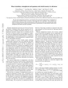
Figure 1: Schematic representation of KPZ interfaces with a positive non-linearity in the presence of upper (MN1) and lower (MN2) walls respectively. The walls are depicted as rigid lines (corresponding to p → ∞; for finite values of p the walls become exponential cutoffs). Observe the difference between the two cases: while in one of them the constant driving force pulls the interface away from the bounding wall (MN1), in the other, the interface is pushed to the wall (MN2).

(pushes) the interface from (against) the wall, while the constant term, acts in the opposite direction in order to keep the interface pinned. These are the two only mechanisms driving the interface average velocity, which imposing stationarity is given by h∂t hi = 0 = ±a ± hb e∓h i + hD(∇h)2 i. (8) At the critical point he∓h i = 0 and, therefore, a has to compensate hD(∇h)2 i. Let us now consider a flat interface ((∇h)2 = 0) at the critical point. While in one case the constant drift, a, pulls it from the wall, causing an effective repulsion from it, in the other one the flat piece is pushed against the wall, being therefore stable (see figure 1). This mechanism leads to essentially different stationary probability distributions in both cases, and ultimately to different universality classes [21]. The limit p → ∞ describes a hard (impenetrable) wall: the interface cannot cross the h = 0 limit in either the upper (h(x, t) < 0) nor the lower wall case (h(x, t) ≥ 0). As we will show the “hardness” (or rigidity) of the wall is not a relevant feature. Indeed, p can be reabsorbed from the KPZ-like equation by modifying the Cole-Hopf transformation to a more general form: φ = exp(mh), where m is a conveniently chosen constant. 2. Directed polymers in random media (DPRM) [33]. 7

The connection with directed polymers in random media has also been known for some time. Indeed, the partition function of the DPRM can be easily seen to obey the following equation (imaginary time Schr¨odinger equation) [33] ∂t Z(x, t) = [D∇2 + η(x, t)]Z(x, t)

(9)

including both: an elastic term (diffusion) and a random potential. Therefore any problem in which the possible values of the DPRM free energy, F ∝ ln Z are restricted, owing to some unspecified reason, from above or from below, can be mapped into a MN equation, or into the KPZ equation with an upper or lower wall respectively. In particular, it has been pointed out by Hwa and coauthors that algorithms used routinely in molecular biology for sequence local-alignment are straightforward realizations of DPRM with a free-energy constraint and are related to the KPZ-problem with a lower wall [36, 21]. Other problems in condensed matter physics, in which a Schr¨odinger equation appear including a random potential, can be ascribed to this class; this can include problems related to Kerr dielectric guides, propagation of optical pulses, multi-channel optical fiber networks, etc. See [13] and references therein. 3. Noisy Burgers equation of turbulence [37, 33]. Considering a KPZ equation and transforming v(x, t) = ∇h(x, t) one obtains the (noisy) Burgers equation describing a randomly stirred vorticity-free (i. e. ∇ × v = 0) fluid dv ≡ ∂t v + v · ∇v = 2∇2 v + ∇η (10) dt where we have fixed D = 2 to ensure invariance of the total derivative under rescaling [33, 34]. The presence of an extra upper wall generates an additional term which cancels out high velocities. This velocity constraint can mimic the role of viscosity in some problems in fluid-dynamics.

4

Properties of Multiplicative Noise. The MN1 class

In this section we explore the phenomenology associated with MN1 by employing different levels of approximation and tools.

4.1 Zero dimensions An exact solution of the one-variable (zero-dimensional) case was provided by Graham and Schenzle [38] (see also [8] and [30] for a review). Indeed, the stationary solution of the associated Fokker Planck equation can be easily worked-out

8

(see Appendix B) Pst (φ) =

1 φ1+2a/σ

2

exp

!

−2bφp−1 . σ 2 (p − 1)

(11)

Let us just underline two curious non-trivial properties of this solution [38]: • All the moments scale in the same way(!) For example, for p = 2 it is just a matter of algebra to obtain m

m/2

hφ i = 2

"

#

h i m + a/σ 2 Γ Γ −a/2σ 2 , 2

(12)

and, therefore, βm defined by φm ∼ |a−ac |βm is equal to unity (1/(p−1) for an arbitrary p) for all m [38, 19]. This is a rather extreme case of anomalous scaling, having its roots in the fact that the asymptotic behavior is controlled by large rare events [39, 40]. • The susceptibility (response to an external field) diverges not only at the critical point, but in a finite interval in the absorbing phase, and the associated critical exponent varies continuously [19].

4.2 Mean Field approaches Developing a consistent and well defined mean-field approximation of Eq.(1) is not a trivial task [22]. It has been only recently that Birner et al. (completing some previous partial results [22]) have shown that [41, 42] σ2 1 , β1 = sup p − 1 2D

!

.

(13)

This result can be obtained by approximating the Laplacian in the Langevin equaP tion by its mean field analog, N1 ∀i (φ(i, t) − φ(x, t)) = hφi − φ(x, t), writing the equivalent Stratonovich (see Appendix A) Fokker-Planck equation σ2 ∂φ (φ∂φ [φP (φ, t)]) 2 (14) and then solving it self-consistently in the stationary limit (see [41] and [9, 22, 42]). Let us underline the non-trivial nature of the mean-field result Eq.(13): for high noise-intensities it does not coincide with the zero-dimensional β (previously called β1 ) exponent β = 1/(p − 1), as usually occurs. Therefore, coupling to ∂t P (φ, t) = ∂φ ([aφ + bφp − D(hφi − φ)]P (φ, t)) +

9

the neighbors is a key ingredient to build up a sound mean-field description. At a field theoretical level (see next subsection) no systematic naive-power counting analysis or tree level approximation has succeeded so far in reproducing the nontrivial result of Eq.(13) (see [22]). Other critical exponents, can be easily computed as usual in mean-field theory. They are defined through τ ∼ ∆ν⊥ , ξ ∼ ∆νk , hφi ∼ t−θ , or τ ∼ ξ z , with τ (ξ) being the correlation time (length), and ∆ = |a − ac | the distance to the critical point. In the current mean field approximation: ν⊥ = 1, νk = 1/2, θ = β = sup{1/(p − 1), σ 2 /(2D)}, and z = 2.

4.3 Beyond Mean Field - Perturbative expansion In order to properly incorporate fluctuations and go beyond mean field, as usual, one has to resort to perturbative expansions combined with renormalization group (RG) techniques [24, 43]. This can be done either directly at the Langevin-equation level, or alternatively working with the corresponding generating functional. Here, contrarily to [19] we choose to employ the second of these frameworks. The generating functional associated with Eq.(1) 10 is [24]: Z[J, H] = DφDψ exp(−S[φ, ψ, J , H]) S=−

R

dd x

R

2

dt[ σ2 φ2 ψ 2 − ψ[∂t φ + aφ + bφp − D∇2 φ] − Jφ − Hφ] (15)

where ψ is a response field, J and H sources coupled to the order parameter field, φ(x, t), and to the response field, ψ(x, t), respectively 11 . Naive power counting shows that the upper critical dimension, below which mean field results cease to be valid, is dc = 2 12 . Following standard perturbative techniques, one can perform an ǫ-expansion below dc . The noise amplitude is written in dimensionless form as σ 2 ≡ uµǫ , where µ is an arbitrary renormalization scale (for example µ2 = a). In −1 momentum-frequency space the propagator is (−iω + a + κ2 ) (for simplicity we fix here D = 1) and the noise vertex is σ2 10

Here we use the Ito representation, as for it the Jacobian of the employed transformation and the theta function evaluated at 0 can be seen to be equal to 1 and 0 respectively, simplifying the algebra [43]. The calculation would be almost identical in the Stratonovich representation, leading to essentially the same results, except for a shift in the critical point. 11 This functional can be easily worked out, by writing the probability of a given time-sequence realization of the noise as a product of Gaussian noise distributions at each time, generating in this way a path integral. Then variables have to be changed from η(x, t) to φ(x, t), and finally a dummy (ghost) variable ψ is introduced by means of a Gaussian transformation, in order to avoid singularities typically induced by the MN. Afterwards the sources J and H are introduced by hand. The process is rather standard; a detailed description can be found in [24] or [43]. 12 This result is easily obtained by imposing the noise term coefficient to be dimensionless at dc .

10

The vertex (ψφp ) is like the previous one but with only one wavy line and p straight ones. It is easy to see that there are no perturbative corrections to the propagator, and the only possible diagrammatic corrections to the noise vertex have the following structure 2 σR = σ2

+ σ4 + σ6 + σ8

+ ... σ2

= 1 − σ2

2

2 = σ which can be written as σR 1−σ2 I where I denotes the one loop diagram at zero external frequency and momenta, and µ2 = a

1 I= (2π)(d+1)

Z

dd κ dω

µ−ǫ 1 1 = α iω + κ2 + µ2 −iω + κ2 + µ2 ǫ

(16)

with α = 2/(8π)d/2 Γ(2 − d/2) [24, 43, 44]. The pole 1/ǫ captures the presence of an infrared singularity below d = 2. For d > 2, I is finite (i. e. it is infrared convergent) 13 therefore if σ 2 is small enough σ 2 I < 1 and the mean-field theory 2; predictions remain valid perturbatively. At σ 2 = I a singularity appears in σR above this noise value the perturbative expansion ceases to be meaningful; usually it is assumed that values of σ 2 > I flow to a non-perturbative fixed point, controlling the long-wavelength large-time asymptotic behavior. For the corrections to vertex ψφp , one has exactly the same structure, except for the rightmost noise vertex (see Eq.(16)) that is replaced by the other one, leading to bR = b(1 + σ 2 I + σ 4 I 2 + ...) =

b 2 = bσR /σ 2 1 − σ2 I

(17)

Therefore, renormalizing σ 2 keeps also bR finite, and no extra renormalization is needed. As the degree of the non-linearity p does not introduce different divergences in the perturbative expansion, it should not affect the critical behavior (as long as p ≥ 2). 13

We assume the existence of a lattice cut-off ensuring the integrals to be ultraviolet convergent.

11

u

DIMENSION

Figure 2: Schematic representation of the RG flow of the dimensionless variable u as a function of dimensionality, as derived from Eq.(1).

Proceeding with the renormalization program, we compute the Wilson β− function defined as β(uR ) = µ∂µ |σ uR = −ǫuR − αu2R

(18)

with a unique physical solution, uR = 0, stable for ǫ < 0 (i. e. above two dimensions) with associated mean field critical exponents. The renormalization-group flow-diagram is very alike the well-known one for KPZ [45, 44], in particular, for d < 2 the flow runs towards infinity for any noise amplitude, while for d ≥ 2 there is a separatrix between the trivial fixed-point basin of attraction and the runawaytrajectories, i. e. between the weak- and the strong-coupling fixed points. Let us emphasize both, the absence of any stable non-trivial perturbative fixed point, and the fact that the theory is super-renormalizable, in the sense that perturbative diagrams have been computed and re-summed to all orders. An alternative derivation of these results can be found in [19]. See also [44] for a very similar calculation presented in a pedagogical way. 14 So far, we have not proven that the strong coupling fixed points in MN (KPZ plus a wall) and KPZ coincide. 15 Observe, however, that right at the critical point the interface falls continuously to minus infinity, as far from the wall as wished. It is therefore very reasonable to assume, that asymptotically, the dynamical exponent 14

It is illuminating to compare the generating functional Eq.(15) with that associated with the reaction A + A → 0 (kink-antikink annihilation) [46, 47, 32, 48]. It has the same structure as (15) but for the sign of the noise term. In terms of the Langevin equation the sign alteration tantamounts to the introduction of a purely imaginary noise [32, 2]. This simple change has dramatic effects, in particular the Wilson β-function is as Eq.(18) but with a positive sign for the quadratic term, generating a non-trivial perturbative fixed point below d = 2 [46], and a different non-trivial physics. 15 It is well known that the KPZ equation should have a strong coupling fixed point controlling its non-trivial physics [44, 34].

12

should be controlled by KPZ scaling (in the absence of the wall). In particular, it can be shown [20] that: (i) the dynamical exponent for MN1 coincides with that of KPZ, (ii) the correlation length exponent, ν (that can be defined for MN but does not exist for KPZ, lacking of a critical point) can be related to the z exponent in KPZ by ν = 1/(2z − 2), and (iii) the order-parameter critical exponent β has to obey β > 1. The reader interested in the proof of these properties is deferred to [20] and to [30] for a more detailed explanation. 4.3.1

Large N limit

Exact RG calculations can be performed in the large N limit for the O(N)-symmetric version of the MN equation defined as ∂t φα (x, t) = −aφα − b|φ|2 φα + D∇2 φα (x, t) + σ|φ(x, t)|ηα (x, t),

(19)

where φ(x, t) = {φ1 , φ2 , ..., φN } is an N-component real vector field, and η is a noise vector field. The cubic term is necessary in order to preserve the O(N ) symmetry. The continuous symmetry of this model allows for two distinct types of active phases: one that preserves the symmetry and one which breaks it. The first one has hφi = 0 and Q = h|φ|2 /N i = 6 0, while for the second both order parameters are non-zero. The main result of the exact solution presented in [19] is that for d ≤ 2, only the symmetric active phase exists, while for d > 2 both types of active phase can exist: for large values of σ 2 the active phase is symmetric, while a broken-symmetry state emerges below a certain critical value of σ 2 . There is also a multicritical point at which the two active and the absorbing phase join (see [19] for more details). At d = 2 a Kosterlitz-Thouless type of transition could appear [50].

4.4 Microscopic models and Numerics Given the lack of analytical tools allowing for a determination of critical exponents in the strong coupling regime, one has to resort to numerical analysis. The first estimation of critical properties was obtained in [20] by discretizing Eq.(1) and performing a numerical integration in d = 1. A more complete study was presented afterwards in [22] in which the two- and three-dimensional cases were also analyzed. In what respect to discrete, microscopic realizations of this universality class, amenable to be simulated, let us remark that any of the many discrete models in the KPZ class reported in the literature [33, 35, 34] is, in principle, susceptible to be modified by introducing a limiting wall, which induces a phase transition. If the non-linearity sign (that can be numerically determined by performing velocity 13

measurements of tilted interfaces [34]) is positive (negative) an upper (lower) wall is required to construct a model in the MN1 class. To the best of our knowledge, at least three different discrete models with these requirements have been studied in the literature [21, 51, 52]. In finite size analysis of Eq.(1) 16 one starts with homogeneous initial conditions, and first determines hφi as a function of the system size, L, for different control parameter values. In a double-logarithmic plot the critical point corresponds to the straight line separating curves bending upward (pinned phase) from downward-bending ones (depinned phase). In order to have a well defined pinned phase for small systems one has to restrict the statistics to pinned runs (otherwise, the only true stationary state for finite systems is the depinned or absorbing one [28, 29, 30]). In systems with MN one has to define a criterion to decide when a configuration is depinned. Numerical results should not (and do not) depend on such a criterion. From the slope of log(φ) versus log(t), one extracts θ = β/νk (see Fig.(8) to have a glance at how finite size scaling graphs look like). From the scaling of saturation values at criticality for different L one obtains β/ν⊥ . Considering a large system size it is possible to obtain β from the scaling of saturation values at various distances from the critical point. In what respect the dynamical exponent, z, it can be determined either from studies of the two-point correlation function at criticality [20] or from spreading experiments [21, 22] 17 . Using spreading experiments at criticality the exponents δ and η, associated with the surviving probability and evolution of the total number of pinned sites respectively, can also be measured [28, 29, 30, 31]. In Table 1 we list the values reported so far in the literature for d = 1. Even though there is some dispersion in the data, and a high precision determination of critical exponents is still lacking, the existence of universal values is firmly established. In d = 3 the two different universality classes predicted by the RG calculation (see Fig.(2)) can be easily recognized: for small σ values very close to mean field expectations have been reported [22] while, for a larger σ non trivial exponents have been found [22] (see Table 2).

4.5 Realizations Among the physical realizations of this class, probably the most relevant one is a rather generic class of synchronization transitions in extended systems (see section 8.2) [17, 54, 52, 55, 56]. 16

See [53] for a review of numerical methods designed to deal with stochastic equations. In spreading experiments φ(x) = 0 at time t = 0 at every single sites, except for a seed-site. See [28, 29, 30]. 17

14

MN [20] Hwa [21] MN [22] RSOS[52] Exact

β 1.70(05) 1.50(15) 1.50(05) 1.69 >1

ν⊥ 1.03(05) ≈1 1.0(1)

β/ν⊥ 1.65(10) 1.55(15) 1.50(10)

1

z 1.53(07) 1.50(05) 1.52(03)

θ 1.10(05) 1.10(12) 1.10(10) 1.19

η

-0.4(1)

1.5

Table 1: Critical exponents measured for the MN1 class in d = 1. RSOS stands for “Restricted solid on solid” model [52]. MN stands for simulations performed directly on the Langevin equation

Weak c. [22] Strong c.[22] Mean Field

β 0.97(05) 2.5(1) βmf

ν⊥ 0.50(5) 0.75(3) 1/2

β/ν⊥ 1.94(2) 3.3(3) 2βmf

z 2.00(0.5) 1.67(03) 2

θ 1.0(1) 2.0(1) βmf

η −0.10(05) −0.5(1) 0

Table 2: Critical exponents measured for the MN1 class in d = 3, for both the weak and the strong coupling regime [22]. Simulations were performed directly in the Langevin equation with p = 2. The two different regimes are obtained by fixing the noise amplitude to a small and a large value respectively; see [22] for further details. βmf is given by Eq.(13). Another important application is in growing interfaces with both adsorption and evaporation of particles on a substrate. This may lead to pinning-depinning transitions or to non-equilibrium wetting transitions [51, 57, 58, 59] (see 8.1). It might also be related to the delocalization transition in an adsorption-reaction model reported in [60]. In reaction-diffusion systems, many times it is possible to derive a Langevin equation in an exact way. In many cases, a multiplicative noise appears, but many times it is purely imaginary! (see the last section of this review refmix, and the references cited there), leading to a completely different phenomenology.

5

The MN2 class

As already anticipated keeping the KPZ non-linearity to be positive, the presence of a lower wall leads to a MN equation including an extra term with respect to the previously studied case: Eq.(6). It has a phenomenology substantially different from

15

that of MN1, Eq.(1). In this section we underline the analogies and differences between these two cases by going through the different levels of approximation discussed in the previous section.

5.1 Zero dimensions The zero-dimensional case is obviously identical to the one for MN1.

5.2 Mean Field approach Concerning the mean field approximation, the average value of the lower-wall extra term, −2D(∇φ(x, t))2 /φ(x, t) generates an exponential non-integrable singularity, ∝ exp(+hφi2 /φ2 ), at the origin of the quasi-stationary potential, solution of the associated Fokker-Planck equation, rendering it non-integrable. Only the depinned (absorbing) phase exists within this approximation. A discussion of different types of mean-field approaches, all of them leading to this same conclusion can be found in [62].

5.3 Beyond Mean Field - Perturbative expansion The additional term −2D(∇φ)2 /φ is non-analytical at φ = 0, rendering unfeasible any type of perturbative expansion. Renormalization group results analogous to those presented for the MN1 class are therefore not available. The arguments leading to ν = 1/(2z − 2) obtained for MN1 can be extended to this case, but the one leading to β > 1 cannot. Indeed, as shown below, in this case ν ≈ 1 as expected, and β takes a value not far from 1/3.

5.4 Microscopic models and Numerics In what respects numerical results, direct simulations of Eq.(6) are hopeless owing to the presence of the singular term. Contrarily, simulations performed in the KPZ representation are feasible, although they are also hard-to-deal-with as is generically the case when discretizing KPZ-type of equations [61]. At the light of this barren perspective, one has to resort to simulations of microscopic models. The first study was that of [21], where critical exponent close to those of the zero-dimensional case were reported, using a well known KPZ-like model [21, 35]. However, it has been recently shown that the results reported in [21] correspond to effective exponent values computed in a transient regime 18 , 18

Apart from the numerical estimates, the rest of the discussion presented in [21] about the differences between the upper and the lower wall cases remains valid.

16

Hwa [62] RSOS [62]

β 0.32(3) 0.325(5)

ν⊥ 0.97(5) ≈1

β/ν⊥ 0.33(2) 0.33(2)

z 1.55(5) ≈ 1.51

θ 0.215(15) 0.21(1)

η 0.80(2)

Table 3: Critical exponents for the MN2 class in d = 1, as measured in two different models: model 1 stands for the one described in [21], and Model 2 is a RSOS one. See [62] for more details. and new accurate values have been measured (results are listed in Table 3 [62]). These studies are performed: (i) using a restricted solid-on-solid (RSOS) model [33, 34, 35, 52] known to belong, in the absence of a wall, to the KPZ class, and reaching system sizes as large as 220 , and (ii) the model considered in [21] but with much larger statistics and performing finite size scaling analyses 19 . Results for both models coincide within errorbars as shown in Table 3. These values are clearly different from those reported for the upper wall, confirming once again the dramatic (ever-surprising) difference between the two classes, as well as the existence of the robust MN2 class itself. The situation is much less satisfactory here than it is for the MN1 class. We have found problems both in mean field and in field-theoretical approaches, and even the numerical integration of the Langevin equation, in either the density of the interface representation is problematic [62] This calls for the development of new analytical tools aimed at tackling this problem and clarifying the physics of this (well identified and robust) universality class.

5.5 Realizations The problem of probing the alignment of different DNA sequences is of outmost importance in molecular biology. One of the most widely used algorithms for such a problem is due to Waterman [36]. Hwa and collaborators, showed that such an algorithm can be mapped onto a KPZ problem with a lower wall (in particular, to its DPRM counterpart) [36]. Locating the critical point of such a transition is what is effectively done by molecular biologists when tuning parameters (i. e. choosing a scoring scheme) to enhance or maximize fidelity in local alignment studies [36]. The MN2 class appear also in some pinning-depinning or non-equilibrium wetting transitions in which a KPZ interface (with positive non-linearity) grows from a substrate [51, 21]. 19

The discrete model considered in [51] is extremely slow to simulate, as exhibits manifestly severe crossover effects.

17

It is known that one-variable MN processes under various circumstances (as, for example, the presence of reset events) lead to generic scale invariance [40, 63, 64]. The MN2 equation is the natural extension of this phenomenon to extended systems, and has been proposed, for instance, to describe the properties of city growth [65, 64], where fluctuations in population number are multiplicative and, obviously, bounded from below.

6

Changing the potential: MN1 with an attractive wall

Up to now we have dealt with Langevin equations describing continuous transitions in systems with MN. In the same way as the Model A for Ising like transitions Eq.(2) has to be modified to the following Langevin equation ∂t φ(x, t) = −aφ − bφ3 − cφ5 + D∇2 φ(x, t) + ση(x, t).

(20)

with b < 0 and c > 0, in order to describe discontinuous, first-order, transitions (in the absence of external magnetic fields) one might wonder what is the MN version of Eq.(20) and what type of physical problems could it represent. To explore this possibility one just needs to change the potential in Eq.(1) to allow for discontinuous jumps: δV (φ) + D∇2 φ(x, t) + σφ(x, t)η(x, t) δφ a b c V (φ) = φ2 + φ3 + φ4 2 3 4

∂t φ(x, t) = −

(21)

with b < 0 and c > 0. If φ ↔ −φ symmetry is to be respected, the simplest potential becomes aφ2 + bφ4 + cφ6 (with no essential difference in the underlying physics). Transforming Eq.(21) to the interface language: ∂V (h) + D∇2 h + D(∇h)2 + ση(x, t) ∂h V (h) = a h + b eh + c/2 e2h .

∂t h(x, t) = −

(22)

For b < 0 this is a KPZ equation in the presence of an attractive upper wall, i. e. in order to depin a site close to the wall, a certain potential barrier has to be overcome. Indeed, the potential V (h) has a local minimum nearby the wall (see Fig.(3). In analogy with the previous sections, this KPZ equation with a positive non-linearity and an upper wall is fully equivalent to a negative non-linearity equation with an attracting lower wall. Eq.(21) is therefore the b < 0 counterpart of the MN1 class. This equation has been studied in different contexts in the literature. It was first proposed by M¨uller et al. [66] to study first order non-equilibrium 18

15

a=0, b=3, c=1

V( h )

10 5 0

a=0, b=-3, c=4

-5 -10

a=0, b=-3, c=1 -2

0

2

4

6

-h Figure 3: Effective potential in terms of h for different parameter values. For b < 0 it has a minimum nearby the wall.

transitions in extended systems. Afterwards, a very similar equation was proposed by Zimmerman et al. [67] as a simplified stochastic model of spatio-temporal intermittency, and by Giada and Marsili [42] to study the effect of Morse potentials in KPZ dynamics 20 . Also, in an interesting paper, Hinrichsen et al. [68] studied what they called first order non-equilibrium wetting: a discrete random deposition model, known to be described by KPZ, in the presence of both evaporation (i. e. a drift) and a limiting attractive substrate (i. e. the motion of the KPZ interface is not just limited by the wall, but the wall is “sticky” in the sense that sites attached to the wall need to overcome an extra potential-barrier in order to become depinned) was analyzed. It can be easily argued [68] that this discrete model is represented at a continuous level by Eq.(21). Following the same steps as in preceeding systems we now analyze Eq.(21) employing different methods.

6.1 Zero dimensions In zero dimensions, the problem is exactly solvable. Thestationary  probability dis−2 2

bφ+ cφ

2

2 1 σ . At the transition tribution being (see appendix B) Pst (φ) = 1+2a/σ 2e φ the order parameter jumps discontinuously from 0 to a non-vanishing value.

6.2 Mean Field approach At a mean field level, we can perform a calculation analogous to that presented for Eq.(1). The numerical solution of the corresponding self-consistency equation 20

Observe that V (h) has the form of a Morse potential.

19

4 2

b -2 -4

Depinned phase

Pinned phase

0

Phase coexistence -6 0

0.5

a

1

1.5

Figure 4: Phase diagram derived from the numerical integration of the mean field approximation of Eq.(21). In the coexistence regions both, the pinned and the depinned solutions are stable, and their edges (marked by dashed lines) correspond to discontinuous transitions, i. e. one of the phases loses its stability abruptly. The transition corresponding to the upper one, ac (b) (signaling the limit of stability of the pinned phase), may become continuous once fluctuations are considered, as discussed in the text.

generates the phase diagram shown in Figure (4). We describe now the main features (for a more detailed explanation see [66, 42, 57, 58]). For positive values of b the transition occurs at a = 0, it is continuous and very similar to the one in Eq.(1): it is in the MN1 class 21 . Instead, for b < 0 the transition bifurcates: there is a discontinuous transition at a = 0, and a second transition (also discontinuous at mean field level) appears at a positive value of a (see Fig.(4)), ac (b). At this value, the pinned phase, hφi = 6 0, loses its stability and falls in an abrupt way to the depinned phase φ = 0. The depinned phase loses its stability at a smaller value a∗ = 0. Therefore, in the interval [0, ac (b)] both solutions are stable: we are in the presence of phase coexistence. The existence of broad coexistence regions is a trait specific of non-equilibrium phase order transitions, and have been reported to appear, among others, in the Toom model [69]. Observe that both of the limiting lines of the coexistence region are discontinuous transitions at this level.

6.3 Beyond Mean Field - Perturbative expansion The theory can be treated perturbatively in a very similar way to Eq.(1); indeed the Feynman diagrams have the same topology in both cases. The new constant c renormalizes as cR = c(1 + σ 2 I + σ 3 I 2 + ...) = 1−σc 2 I and a RG flow analogous to that for Eq.(1) is obtained. The only difference is that now as long as 21

As in MN1, in this case, for a > 0 (a < 0) the tail of the potential would attract (repel) distant interfaces to (away from) the wall; the transition from one case to the other occurs at a = 0.

20

the transition is discontinuous (not scale invariant) the trajectories for large enough noise amplitudes (above the separatrix in Fig.(2)) are not expected to flow to a strong coupling fixed point, but to be runaway trajectories. In any case, there is no non-trivial stable fixed-point and, consequently, standard perturbative expansions cannot say anything about the strong noise regime.

6.4 Microscopic models and Numerics Eq.(21) has been studied numerically in different contexts [67, 42] and recently in [57, 58]. Its main properties (described mainly in the interface language) are as follows. The mean-field phase-diagram qualitative-structure survives the inclusion of fluctuations, namely: 6.4.1

b>0

For b > 0 a continuous phase transition is observed. This transition has been extensively verified to belong to the MN1 class [57, 58]. 6.4.2

b0 λ0 λ 0 case i. e. to the MN2 class.), while for sufficiently large ones, it remains first order without a broad coexistence region 28 . In this way, the presence of fluctuations may drive the transition from discontinuous (at mean field level) to continuous in some parameter range. In other words the tricritical point is shifted from b = 0 at mean field, to a negative value when fluctuations are taken into account (this effect is much stronger here than it is in the previous case). This result has been verified in numerical simulations both using the model in [21] and a RSOS model in the presence of an attractive wall [62]. Let us stress again that even if the transition is discontinuous, first-order, in the strong attraction regime, it does not involve a broad coexistence region nor a region of STI as occurred in the ∂t φ(x, t) = −aφ − bφ2 − cφ3 + D∇2 φ(x, t) − 2D

27

We have to admit that this looks like a tongue-twister and we humbly suggest the long suffering reader to draw a diagram to clarify the list of possibilities. This diagram should include 23 situations: upper or lower wall?, positive or negative non-linearity?, attractive or non attractive wall?; and only 4 different physical behaviors, described respectively by this and the 3 preceeding sections. Table 4 and Fig. (9) should be of some help. 28 Observe that the first-order transition here does not require the presence of coexistence between active and absorbing phases: it just corresponds to the point where the free interface has zero velocity, and therefore does nor contradict Hinrichsen’s claim [49].

28

previously discussed case. The transition is located for any value of b at the point where the depinned phase (free interface) looses its stability. One way to rationalize this result (and its being at odd with the previous section one) is as follows. In the MN1 class in which there is an effective repulsion from the wall as discussed at the beginning of the paper, the introduction of attractiveness has a profound effect. In particular, two opposite physical mechanisms compete: one repelling sites from the wall and the other attracting them to it. This is at the origin of the existence of a broad coexistence region. Contrarily, for the MN2 class such an effective repulsion does not exist and, therefore, introducing attractiveness is a much milder perturbation in this case. Indeed, it does not alter nor the order nor the exponents of the transition that remains in the MN2 class for sufficiently small values of |b|, and it induces a standard discontinuous transition (no broad coexistence region) for large enough (very strong) attractiveness. A similar phase diagram, including first and second order transitions as well as a tricritical point separating them, has been reported by Hinrichsen et al. in their discrete non-equilibrium wetting model, for parameter values corresponding to the case under consideration.

8

Applications: Non-equilibrium wetting and synchronization

In this section we briefly review two of the main fields in which the formalism and results of the previous sections can be straightforwardly applied: non-equilibrium wetting and synchronization in spatially extended systems. We discuss how MN equations as those described in the preceeding sections come out within these contexts.

8.1 Non-equilibrium Wetting When a phase (α) is in contact with a substrate, wetting occurs if a macroscopic layer of a coexisting phase (β) is adsorbed at the substrate. The wetting transition is characterized by the divergence of the β-layer thickness; the αβ interface goes arbitrarily far from the substrate. Equilibrium wetting is a problem of great experimental as well as theoretical importance. It has been extensively investigated using interface displacement models, in which h(x, t) represents the interface distance from the substrate [80]. The minimal dynamical (equilibrium) wetting model is given by the following Edwards-Wilkinson (EW) [81] Langevin equation [82] ∂t h(x, t) = D∇2 h − 29

∂V + ση(x, t). ∂h

(25)

This was introduced by Lipowsky [82], and describes the relaxation of h towards its equilibrium distribution, specified by V (h). A physically motivated choice for the interaction potential has the following form (Morse potential) [80] V (h) = b(T )e−h + ce−2h

(26)

where b(T ) vanishes at the wetting temperature and c > 0. At sufficiently low temperatures, b < 0, the potential V binds the αβ interface; the equilibrium thickness of the wetting layer hhi is finite. As the temperature is raised, the potential becomes less attractive and at some point it no longer binds the interface, hhi diverges. In order to study complete wetting (i. e. wetting occurring in the limit in which the chemical potential difference between the two phases, µ, goes to zero for T larger than the wetting-temperature) a linear term µh has to be added to V (h) [80]. µ plays the role of an external force acting on the interface. The dynamic model, Eq.(25) is readily generalized to non-equilibrium interfacial processes, e.g., crystal growth, atomic beam epitaxy, etc., where thermal equilibrium does not apply. This has been done in detail in [57, 58, 59]. 29 The conclusion is that the most basic effective non-equilibrium interfacial model consists of a KPZ equation (instead of Eq.(25)) in the presence of a substrate, i.e.: the MN equation. The origin and nature of the KPZ non-linearity within this context has been discussed in [57, 58, 59]. A detailed discussion about non-equilibrium critical wetting, complete wetting, the difference between pinning-depinning and wetting-dewetting transitions, and other related issues can be found in [58, 59] (see also [83]).

8.2 Synchronization Mutual synchronization of oscillators is one of the most intriguing and fascinating phenomena appearing in complex systems [84, 85]. Some examples appear in chemical reactions [86], neuronal networks [87], flashing fireflies [88], Josephson junctions [89], and semiconductor lasers [90] to mention but a few. See [84] for an elementary introduction to this growing field and [85] for an excellent review. Coupled map lattices (CML) [91, 92] have attracted much attention as a paradigm in the study of synchronization in spatially extended systems under mathematical grounds. When two replicas of a same CML are locally coupled [55, 93], or when they are coupled to a sufficiently large common external random noise even if they are not coupled to each other [94, 95, 54], they can achieve mutual synchronization. In all the aforementioned examples, there is a transition from a chaotic or unsynchronized phase, in which the differences between both replicas persist, to a 29

See also [51, 68] where the same problem was first studied for discrete models.

30

synchronized one in which memory of the initial differences is erased and replicas synchronize with certainty. The analysis of universal properties of synchronization transitions (ST) has been the subject of many recent studies [55, 56, 54, 17, 52]. In particular, as mentioned previously, in a seminal paper, Pikovsky and Kurths devised a method to map the synchronization error field (i. e. the difference between two replicas) into the MN equation 1. On the other hand, it was proposed that for discrete systems the ST should be in the DP class [55, 56]. Based on recent observations [54, 52, 95] a global picture, that can be synthesized as follows, has emerged: there are two types of ST depending on whether the largest (transverse) Lyapunov exponent, Λ, is zero or negative right at the transition [54, 52]. In the first case, the transition is MN like, and it is controlled by linear stability effects (i. e. Λ changes sign at the transition). In the second group the transition is either DP or discontinuous depending on microscopic details (and the transition is located where the propagation velocity of non-linear perturbations changes sign, while Λ is negative). This situation is in complete analogy with what reported for Eq.(21). Indeed, as shown in [18], a straightforward generalization of the derivation by Pikovsky and Kurths leads to Eq.(21) instead of Eq.(1) in the cases when there is some singularity or discontinuity in the local map. 30 In particular, as discussed in [18] if there is a typical re-injection rule or another mechanism leading to a typical value of the local synchronization error field, then the corresponding potential in the Langevin equation needs to have a local minimum, and therefore, the structure of Eq.(21) rather than Eq.(1). In conclusion, Eq.(21) is the minimal Langevin equation describing ST in a general way. All the so-far reported universality classes in one-component synchronizing system are describable by this equation, and consequently belong to one of the three classes reported for it: MN1, DP or are discontinuous. See [18] for further details and analysis.

9

Miscellaneous comments

We present some miscellaneous remarks on issues related to the ones discussed along this paper; they might be of some interest in order to get a global picture of the state of the art. See also the recent review [97]. • Negative Diffusion 30 In a recent paper [96] it has been shown how DP can emerge in synchronization transitions, even for some continuous maps.

31

By considering negative values of the diffusion constant, anti-ferromagnetic ordering can be studied. In particular, Birner et al. [41] have recently studied a MN equation with p = 3. They consider both positive as well as negative values of the order parameter field and report on an anti-ferromagnetic MN phase transition (in the MN1 class). • Additive Noise The presence of additive noise in an otherwise MN changes the universality of the transition [9, 15, 16]: it is a relevant perturbation from the RG point of view. This is easily checked as the additive noise is more relevant from naive power-counting analysis than the multiplicative one. The phenomenon of reentrance may appear when both multiplicative and additive noises act together: the system can become more ordered by increasing the MN amplitude, but eventually the additive part will take over, disordering the system [15, 16]. For example, it has been shown that annealed Ising models, known to have a reentrant transitions can be described by Langevin equations with competing additive and multiplicative noises [98]. • Colored Noise One can wonder what is the effect of colored noise in MN type of equations. From the RG point of view deviations from Gaussianity in the noise are irrelevant, but they might have some effects on the phase diagram (see for instance [99, 100]). In [101] the effect of spatially oscillating MN has been studied. • Higher order Noises Having studied Langevin equations with minimal potentials and noises amplitudes proportional to φ0 , φ1/2 , and φ1 , one might wonder if higher powers, as for instance 3/2 or 2 have any physical significance. If one construct using standard Fock space techniques [48] an effective Langevin equation (or equivalently a generating functional) for reaction diffusion process occurring in n-plets (triplets, quadruplets, etc), it is easy to see that they generate noise amplitudes proportional to φn/2 If all possible reactions in a given system require the presence of triplets, it is reasonable to expect a 3/2 type of noise [79, 102]. For a general n − plet process a noise amplitude proportional to φn/2 is expected to be the leading contribution. This could generate new universality classes not fully explored yet. See also [103] where other noise terms are studied. • Long range interaction 32

If one considers long-range (for example, van der Waals) interactions between the substrate and the interface in the wetting problem the potential has the general form [104, 80] V (h) = b(T )h−m + ch−n ,

n > m > 0.

(27)

A similar interaction has been recently used to describe a class of synchronization problems for which a new universality class has been claimed to appear [105]. We are presently working in this problem. • Quenched disorder The presence of quenched disorder is known to generate new non-trivial phenomenology in both Ising and DP -like systems. It is also expected to be a relevant perturbation at the different MN universality classes reported here. Its analysis and relation with physical processes, as localization, is currently under investigation. • Multicritical Points At the points where different critical lines meet, a different, multicritical behavior is expected to show up. These multicritical points and their corresponding Langevin representations (most likely including MN) are still to be studied in depth [52, 105]. A multicritical point like these should be related to critical non-equilibrium wetting as described in [58] (see also [83]). • Complex Multiplicative Noise It is well known that certain (annihilation) processes can be represented by a Langevin equation with MN, but a complex amplitude [46, 47, 48, 2, 32, 78]. The degree of validity of such Langevin equations with complex noise still lacks of a satisfactory analysis; see [32, 78] for some discussions of this and related topics.

10 Conclusions We have reviewed different aspects of non-equilibrium phase transitions exhibited by systems amenable to be represented by a Langevin equation with MN. These systems exhibit a phase transition from an absorbing phase to an active one, as for example pinning-depinning transition, non-equilibrium wetting transitions and synchronization transitions. A rich phenomenology can be further explored by exploiting the Cole-Hopf transformation that maps MN systems into non-equilibrium

33

(KPZ) interfaces in the presence of an extra limiting wall. Depending on the position and nature of the wall we have identified and characterized up to 4 different types of critical behavior that are synthesized in Table 4. It is our hope that this review will foster new developments in the fields of nonequilibrium phase transitions and systems with MN, and stimulate the application of these ideas to other open problems in physics and in other disciplines.

Appendix A: Ito versus Stratonovich Let us consider a MN equation in the Stratonovich representation. Then it is completely analogous to an Ito-interpreted Langevin equation in which the linear coefficient a has to be replaced by a + σ 2 /2 [1, 2]. Therefore, for this type of noise the only difference between Ito and Stratonovich tantamounts to a shift in the control parameter. Along this paper we use both Ito and Stratonovich interpretations, as the results obtained for any of them can be straightforwardly modified to apply to the other. An exception are noise induced transitions as those reported in [9], the difference between Ito-Stratonovich is essential in this case, as the noise amplitude plays a key role in the linear control parameter only if the equation is interpreted a la Stratonovich [16]. See [106] where a new type of noise induced transition is reported to occur for both Ito and Stratonovich interpretations.

Appendix B: The 0-dimensional case. Solution of the stationary Fokker-Planck equation. Comparison with RFT. Let us consider Eq.(1) in the zero-dimensional limit ∂t φ(t) = −aφ − bφp + σφη

(28)

The associated Fokker-Planck equation in the Stratonovich representation is σ2 ∂φ [φ∂φ [φP (φ)]] (29) 2 whose stationary solution (trivially obtained imposing detailed balance) is given by Eq.(11). As long as a > 0 the probability becomes non-normalizable, and the only stationary state is φ = 0. Therefore the transition is located at ac = 0. In the Ito interpretation it is shifted to a = σ 2 /2. Observe that in the absorbing phase the singularity at the origin is non-integrable and changes continuously its degree but, above the critical point, the singularity disappears. Instead, for the RFT noise (i. e. replacing φ by φ1/2 in the noise term), following the same steps one obtains, ∂t P (φ, t) = ∂φ [(aφ + bφp )P (φ)] +

2 φp 1 Pst (φ) = exp − 2 aφ − φ σ p 

34





.

(30)

Here the singularity exists in both the active and the absorbing phase, therefore P (φ) reduces to a delta function at the origin. This reflects the fact that for RFTlike finite systems the only true stationary state is the absorbing one. Different plots, comparisons and discussion of the (pseudo)-stationary potentials for RFT and MN can be found in [32].

Appendix C: The problem of the quenched KPZ Let us consider the problem of a KPZ interface, with a positive non-linearity in the presence of quenched disorder (QKPZ), ξ(x, h), where ξ is a Gaussian distribution. It was proposed in [107] that the scaling properties of this problem at criticality should be controlled by a DP type of fixed point in d = 1 31 . The logic behind this prediction is that the interface is pinned by a path of impurities such that it percolates from one side to the other, blocking the whole interface front. As the path is directed, DP is expected to control its scaling. Observe that, owing to topological reasons the same reasoning does not apply to two dimensional systems. In d = 2 a directed surface is required to block the interface advance. A scaling theory of directed surfaces was proposed in [108] to account for this. Despite of the numerous computational confirmations of the QKPZ-DP connection, no analytical study has succeeded so far in establishing such a link in a more rigorous way. The difficulties stemming from the fact that it seems that the order parameter has to be changed: it is the interface velocity for KPZ, while it should be related to the density of pinning sites in the QKPZ case. Establishing under firm grounds the equivalence between QKPZ and DP remains an open challenging problem. In the case of a negative KPZ non-linearity, simulations show either triangular patterns resembling the ones discussed previously 32 and a first order pinningdepinning transition has been reported to occur [72] or, alternatively, critical properties controlled by DP [109] depending upon model details or parameter values. Let us emphasize the deep analogies between this situation and the one described in Section 6.

Acknowledgments I gratefully acknowledge my collaborators on the issues discussed in this review. I am particularly indebted with Geoff Grinstein and Yuhai Tu, who initiated me into this field and taught me much about this and other issues, and also with 31 To be more precise the QKPZ is believed to be described by directed percolation depinning. See [34] and [33] and references therein. 32 Named “facet” in the context of surface growth.

35

Terry Hwa, Walter Genovese, Margarida Telo da Gama, Pedro L. Garrido, Romualdo Pastor-Satorras, Jos´e M. Sancho, and Abdelfattah Achahbar. I also thank Ron Dickman, Roberto Livi, Luciano Pietronero, Giorgio Parisi, Matteo Marsili, Haye Hinrichsen, Hugues Chat´e, Raul Toral, Pablo Hurtado, Andrea Gabrielli, Claudio Castellano, Francesca Colaiori, and Lorenzo Giada for illuminating discussions. I thank Francisco de los Santos for enjoyable collaborations as well as for a critical reading of the manuscript. My warmest thanks also to the editors, Elka and Rodolfo, for inviting me to participate in this book. Financial support from the Spanish MCyT (FEDER) under project BFM2001-2841 is also acknowledged.

References [1] N.G. van Kampen, Stochastic Processes in Physics and Chemistry, North Holland, Amsterdam, 1981. [2] C.W. Gardiner, Handbook of Stochastic Methods, Springer Verlag, Berlin and Heidelberg, 1985. [3] P.C. Hohenberg and B.I. Halperin, Rev. Mod. Phys. 49, 435, (1977). [4] R. Benzi, A. Sutera and A. Vulpiani, J. Phys. A 14, L453 (1981). K. Weisenfeld and F. Moss, Nature 373, 33 (1995). [5] C.R. Doering and J.C. Gadoua, Phys. Rev. Lett. 69, 2318 (1992). See also, P. Pechukas and P. H¨anggi, Phys. Rev. Lett. 73, 2772 (1994). [6] See J. Garc´ıa-Ojalvo, and J. M. Sancho, Noise in Spatially Extended Systems, Springer, New York, 1999; and references therein. See also, J. M. Sancho and J. Garc´ıa-Ojalvo, in Lecture Notes in Physics 557, p.235, ed. J. A. Freund and T. P¨oschel, Springer-Verlag, Berlin (2000). [7] J. Garc´ıa-Ojalvo, A. Hern´andez-Machado and J. M. Sancho, Phys. Rev. Lett. 71, 1542 (1993); J. M. Parrondo, C. Van den Broeck, J. Buceta and F. J. de la Rubia, Physica A 224, 153 (1996). [8] See W. Horsthemke e R. Lefever, Noise Induced Transitions, Springer Verlag, Berlin, 1984, and references therein. [9] C. Van den Broeck, J.M.R. Parrondo and R. Toral, Phys. Rev. Lett. 73, 3395 (1994). C. Van den Broeck, J. M. R. Parrondo, R. Toral and R. Kawai, Phys. Rev. E 55, 4084 (1997). C. Van den Broeck, J.M.R. Parrondo, J. Armero and A. Hern´andez-Machado, Phys. Rev. E 49, 2639 (1994). 36

[10] See M. A. Cirone, F. de Pasquale, B. Spagnolo, Int. Journal of Fractals (2001); Cond-mat/010739; and references therein. [11] F. Drolet and J. Vi˜nals, Phys. Rev. E 64, 026120 (2002). [12] G. Tripathy, A. Rocco, J. Casademunt, and W. van Saarloos, Phys. Rev. Lett. 86, 5215 (2001). Phys. Rep. 337, 139 (2000). [13] G. Kaniadakis and A. M. Scarfone, J. Phys. A. 35, 1943 (2002). [14] A. Becker and L. Kramer, Phys. Rev. Lett. 73, 955 (1994). [15] J. Garc´ıa-Ojalvo, J.M.R. Parrondo, J.M. Sancho y C. Van den Broeck. Phys. Rev. E 54, 6918 (1996) [16] W. Genovese, M.A. Mu˜noz and J.M. Sancho, Phys. Rev. E 57, R2495 (1998). [17] A. Pikovsky and J. Kurths, Phys. Rev. E 49, 898 (1994). [18] M.A. Mu˜noz and R. Pastor Satorras, cond-mat/0301059.

Phys. Rev. Lett. (2003).

[19] G. Grinstein, M.A. Mu˜noz, and Y. Tu Phys. Rev. Lett. 76, 4376 (1996). [20] Y. Tu, G. Grinstein and M.A. Mu˜noz, Phys. Rev. Lett. 78, 274 (1997). [21] M.A. Mu˜noz and T. Hwa, Europhys. Lett. 41, 147 (1998). [22] W. Genovese and M.A. Mu˜noz, Phys. Rev. E 60, 69 (1999). [23] M. C. Cross and P. C. Hohenberg, Rev. Mod. Phys. 65, 851 (1993). [24] J. Zinn-Justin, Quantum Field Theory and Critical Phenomena, Oxford Science, Oxford, (1989). [25] J. Cardy, Scaling and Renormalization in Statistical Physics, Cambridge Univ. Press, (1997). [26] J.L. Cardy and R.L. Sugar, J. Phys. A 13, L423 (1980). H.K. Janssen, Z. Phys. B 42, 151 (1981). P. Grassberger, Z. Phys. B 47, 365 (1982). [27] W. Kinzel, in Percolation Structures and Processes, edited by G. Deutsher, R. Zallen and J. Adler, Ann. Isr. Phys. Soc., 5 (Hilger, Bristol, 1983). [28] H. Hinrichsen, Adv. Phys. 49 1, (2000).

37

[29] J. Marro and R. Dickman, Nonequilibrium Phase Transitions and critical phenomena (Cambridge University Press, Cambridge, 1998). [30] G. Grinstein and M. A. Mu˜noz, The Statistical Mechanics of Systems with Absorbing States, in ”Fourth Granada Lectures in Computational Physics”, ed. by P. L. Garrido and J. Marro, Lecture Notes in Physics, Vol. 493 (Springer, Berlin 1997), p. 223. [31] G. Odor, cond-mat/0205644. [32] M. A. Mu˜noz, Phys. Rev. E. 57, 1377 (1998). [33] T. Halpin-Healy and Y.-C. Zhang, Phys. Rep. 254, 215 (1995); and ref. therein. [34] A. L. Barab´asi, H. E. Stanley, Fractal Concepts in Surface Growth Cambridge University Press, Cambridge, 1995; and ref. therein. [35] J. Krug, Adv. in Phys. 46, 139 (1997). J. Krug and H. Spohn, in Solids far from equilibrium, Ed. C. Godreche. Cambridge Univ. Press, (1991). [36] T. Hwa and M. Lassig, Phys. Rev. Lett. 76, 2591 (1996). See also, T. Hwa and M. Lassig, ”Optimal Detection of Sequence Similarity by Local Alignment” in Proceedings of the Second Annual Int. Conf. on Computational Molecular Biology (RECOMB98), S. Istrail, P. Pevzner, and M.S. Waterman eds, 109116 (ACM Press, 1998); and references therein. R. Olsen, T. Hwa and M. Lassig, ”Optimizing Smith-Waterman Alignments” in Pacific Symposium on Biocomputing 4, 302-313 (1999). [37] J. M. Burgers, The nonlinear diffusion equation, Riedel, Boston, (1974). [38] R. Graham and A. Schenzle, Phys. Rev. A 25, 1731 (1982). Schenzle and H. Brand, Phys. Rev. A 20, 1628 (1979). [39] S. Redner, Am. J. Phys. 58, 267 (1990). [40] D. Sornette, Critical Phenomena in Natural Sciences, Springer-Verlag, Berlin, (2000). [41] T. Birner, K. Lippert, R. M¨uller, A. K¨unel, and U. Behn, Phys. Rev. E 65, 046110 (2002). [42] L. Giada and M. Marsili, Phys. Rev. E 62, 6015 (2000).

38

[43] C. J. DeDominicis, J. Physique 37, 247 (1976); H. K. Janssen, Z. Phys. B 23, 377 (1976); P. C. Martin, E. D. Siggia, and H. A. Rose, Phys. Rev. A 8, 423 (1978); L. Peliti, J. Physique, 46, 1469 (1985). [44] See K. J. Wiese, J. Stat. Phys. 93, 143 (1998); and references therein. M. Lassig, J. Phys. C 10, 9905 (1998). [45] M. Kardar, G. Parisi and Y. C. Zhang, Phys. Rev. Lett. 56, 889 (1986). [46] L. Peliti, J. Phys. A 19, L365 (1986). [47] B. P. Lee, J. Phys. A 27, 2633 (1994). [48] L. Peliti, J. Physique 46, 1469 (1985). See also, B. P. Lee and J. Cardy, J. Stat. Phys. 80, 971 (1995). [49] H. Hinrichsen, Condmat/0006212. [50] J.M. Kosterlitz and D.J. Thouless, J. Phys. C 6, 1181 (1973). [51] H. Hinrichsen, R. Livi, D. Mukamel, and A. Politi, Phys. Rev. Lett. 79, 2710 (1997). [52] V. Ahlers and A. Pikovsky, Phys. Rev. Lett. 88, 254101 (2002). V. Ahlers, Ph. D. thesis. http:// www.stat.physik.uni-potsdam.de/ volker/publ.html. F. Ginelli, et al., cond-mat/0302588. [53] M. San Miguel and R. Toral, Stochastic Effects in Physical Systems, to be published in Instabilities and Nonequilibrium Structures, VI, E. Tirapegui and W. Zeller, eds. Kluwer Academic Pub. (1997). (cond-mat/9707147). [54] L. Baroni, R. Livi, and A. Torcini, Phys. Rev. E 63, 036226 (2001). [55] P. Grassberger, Phys. Rev. E 59, R2520 (1999). [56] See, P. Grassberger, in Nonlinearities in Complex Systems, ed. by S. Puri and S. Dattagupta (Narosa Pub. House, New Delhi, 1997), pag. 61. [57] F. de los Santos, M.M. Telo da Gama, and M.A. Mu˜noz, Europhys. Lett. 57, 803 (2002). [58] F. de los Santos, M.M. Telo da Gama, and M.A. Mu˜noz, Phys. Rev. E 67, 021607 (2003).

39

[59] F. de los Santos, M. M. Telo da Gama, and M. A. Mu˜noz, Depinning and wetting in nonequilibrium systems, in “Modeling Complex Systems”, AIP Conf. Proc. 661, 102 (2003). cond-mat/0211124. [60] H. Kaya, A. Kabakcioglu, and A. Erzan, Phys. Rev. E 61, 1102 (2000). [61] T. J. Newman and A. J. Bray, J. Phys. A 29, 7917 (1996). C.H. Lam and F. G. Shin, Phys. Rev. E 58, 5592 (1998). [62] M. A. Mu˜noz, and F. de los Santos, and A. Achahbar. cond-mat/0304239. [63] S. Solomon and M. Levy, Int. J. Mod. Phys. C 7, 745 (1996). R. Cont and D. Sornette, J. Phys. I (France) 7, 431 (1997). H. Takayasu, A.H. Sato, and M. Takayasu, Phys. Rev. Lett. 79, 966 (1997). D. Sornette, Phys. Rev. E 57, 4811 (1998). O. Biham, O. Malcai, M. Levy, and S. Solomon, Phys. Rev. E 58, 1352 (1998). [64] D.H. Zannete and S.C. Manrubia, Phys. Rev. Lett. 79, 523 (1997). See also, S.C. Manrubia and D.H. Zannete, Phys. Rev. E 59, 4945 (1999). [65] M. Marsili, S. Maslov, and Y.C Zhang, Phys. Rev. Lett. 80, 4830 (1998). [66] R. M¨uller, K. Lippert, A. K¨unel, and U. Behn, Phys. Rev. E 56, 2658 (1997). [67] M.G. Zimmermann, R. Toral, O. Piro, and M. San Miguel, Phys. Rev. Lett. 85, 3612 (2000). [68] H. Hinrichsen, R. Livi, D. Mukamel, and A. Politi, Phys. Rev. E 61, R1032 (2000). See also, K. Park and I. Kim, Phys. Rev. E 65, 066106 (2002). [69] A. L. Toom, in Multicomponent Random Systems, ed. by R. L. Dobrushin, in Advances in Probability, Vol. 6, 549, (Dekker, New York, 1980). C. H. Bennett and G. Grinstein, Phys. Rev. Lett. 55, 657 (1985). [70] H. Chat´e and P. Manneville, Phys. Rev. Lett. 58, 112 (1987). H. Chat´e, in Spontaneous Formation of Space-Time Structures and Criticality, ed. by T. Riste and D. Sherrington, p. 273 (Kluwer 1991). [71] H. Hinrichsen, condmat/0302381. [72] H. Jeong, B. Kahng, and D. Kim, Phys. Rev. E 59, 1570 (1999). [73] M. A. Mu˜noz, R. Dickman, A. Vespignani, and S. Zapperi, Phys. Rev. E, 59, 6175 (1999).

40

[74] R. Dickman and J. K. L. da Silva, Phys. Rev. E 58, 4266 (1998). [75] M. Droz and A. Lipowski, cond-mat/0211145. [76] J.F.F. Mendes, R. Dickman, M. Henkel and M.C. Marques, J. Phys. A 27, 3019 (1994). M. A. Mu˜noz, G. Grinstein, R. Dickman, and R. Livi, Phys. Rev. Lett. 76, 451, (1996). M. A. Mu˜noz, G. Grinstein, and R. Dickman, J. Stat. Phys. 91, 541(1998). [77] E. Carlon, M. Henkel, and U. Schollw¨ock, Phys. Rev. E 63, 036101 (2001). ´ H. Hinrichsen , Phys. Rev. E 63, 036102 (2001). G. Odor, Phys. Rev. E 62, ´ R3027 (2000). H. Hinrichsen, Physica A 291, 275 (2001). G. Odor, Phys. Rev. E 63, 067104 (2001). J. D. Noh and H. Park, cond-mat/0109516, (2001). G. T. Barkema and E. Carlon, cond-mat/0302151, (2003). [78] M. J. Howard and U. T¨auber, J. Phys. A: Math. Gen. 30, 7721 (1997). [79] K. Park, H. Hinrichsen, I. Kim, Phys. Rev. E 66, 025101(R) (2002). See also, J. Kockelkoren and H. Chat´e, cond-mat/0208497; and G. Odor, cond-mat/0210615. [80] S. Dietrich, in Phase Transitions and Critical Phenomena, vol. 12, ed. C. Domb and J. Lebowitz, Academic Press (1983); D.E. Sullivan and M.M. Telo da Gama, in Fluid Interfacial Phenomena, ed. C.A. Croxton. Wiley, N.Y. (1986). [81] S.F. Edwards and D.R. Wilkinson, Proc. R. Soc. London A 381, 17 (1982). [82] R. Lipowsky, J. Phys. A 18, L585 (1985). [83] H. Hinrichsen, R. Livi, D. Mukamel, and A. Politi, cond-mat/0304357. [84] S. H. Strogatz and I. Stewart, Scientific American, 269 102, (1993). S. H. Strogatz, Nonlinear Dynamics and Chaos, Addison-Wesley (1994). [85] A. Pikovsky, M. Rosemblum, and J. Kurths, Synchronization: A universal concept in non-linear sciences, Cambridge University Press, 2001. [86] Y. Kuramoto, Chemical oscillations, Waves, and Turbulence, Springer, Berlin (1984). [87] F. C. Hoppensteadt and E. M. Izhikevich, Weakly Connected Neural Networks, (Springer, New York, 1997). E. A. Stern et al. , Nature (London), 394, 475 (1998). R. C. Elson et al. , Phys. Rev. Lett. 81, 5692 (1998). 41

[88] J. Buck, Quart. Rev. Biol. 63, 265 (1988). [89] P. Hadley et al. , Phys. Rev. B 238, 8712 (1988). [90] I. Fischer et al. Europhys. Lett. 35, 579 (1996). G. Giacomelli and A. Politi, Phys. Rev. Lett. 76, 2686 (1996). [91] Theory and Application of Coupled Map Lattices, ed. by K. Kaneko, J. Wiley and Sons, Chichester, (1993). [92] H. Chat´e and P. Manneville, Phys. Rev. Lett. 58, 112 (1987); Prog. Theor. Phys. 87, 1 (1992); Physica A 32, 409 (1988). [93] L. G. Morelli and D. H. Zanette, Phys. Rev. E 58, R8 (1998). A. Amengual, E. Hern´andez Garc´ıa, R. Montagne, and M. San Miguel, Phys. Rev. Lett. 78, 4379 (1997). [94] F. Cecconi, R. Livi, and A. Politi, Phys. Rev. E 57, 2703 (1998). F. Bagnoli and F. Cecconi, Condmat/9908127. [95] F. Bagnoli, L. Baroni, and P. Palmerini, Phys. Rev. E 59, 409 (1999). [96] F. Ginelli, R. Livi, A. Politi, and A. Torcini, Condmat/0212454. [97] M. A. Mu˜noz, Puzzling problems in non-equilibrium field theories. Bulletin of Asia Pacific Center for Theoretical Physics (APCTP), 9-10, 5 (2002). Condmat/0210645. [98] W. Genovese, M. A. Mu˜noz and P.L. Garrido, Phys. Rev. E 58, 6828 (1998). [99] S. E. Mangioni, R. R. Deza, R. Toral, and H. Wio, Phys. Rev. Lett. 79, 2389 (1997); Phys. Rev. E 61, 223 (2000). [100] J. Garc´ıa-Ojalvo, J.M. Sancho y L. Ramirez-Piscina, Phys. Lett. A 168, (1992). J. Garc´ıa-Ojalvo, J.M. Sancho, and H. Guo, Physica D 113, 331 (1998). [101] J. R¨oder, H. R¨oder, and L- Kramer, Phys. Rev. E 55, 7068 (1997). [102] O. Al Hammal, H. Chat´e, and M. A. Mu˜noz, Preprint (2003). [103] S.L. Denisov and W. Horsthemke, Phys. Rev. E 65, 061109 (2002); 65, 031105 (2002). [104] R. Lipowsky, Phys. Rev. Lett. 52, 1429 (84). [105] A. Lipowski and M. Droz, Condmat/0212142. 42

[106] O. Carrillo, M. Iba˜nez, J. Garc´ıa-Ojalvo, J. Casademunt, and J. M. Sancho. Condmat/0302264. [107] L.-H. Tang and H. Leschorn, Phys. Rev. A 45 , 8309 (1992). S. V. Buldyrev et al. , Phys. Rev. A 45 , 8313 (1992). [108] A. L. Barabasi, G. Grinstein, and M. A. Mu˜noz, Phys. Rev. Lett. 76, 1481, (1996). [109] Y. Choi, H. Kim, and I. Kim, Phys. Rev. E 66, 047102 (2002).

43