2008 American Control Conference Westin Seattle Hotel, Seattle, Washington, USA June 11-13, 2008
FrB04.2
Multirate Adaptive Notch Filter with an Adaptive Bandwidth Controller for Disk Drives Jason Levin and Petros Ioannou Abstract— This paper presents the simulation results performed of a multirate adaptive notch filter with adaptive bandwidth controller for disk drives. The resonant modes of a disk drive may be uncertain and vary between units, and can also lie near or beyond the nyquist frequency. Suppressing these modes can be difficult. However, with an adaptive notch filter that is able to accurately track the resonant frequencies, the effects of such modes can be suppressed. By adding a multirate scheme to the adaptive notch filter, it can suppress modes at higher frequencies. As the multirate adaptive notch filter tracks the plant mode frequencies, the adaptive bandwidth controller ensures that stability and performance requirements are satisfied. The simulation results that are included show the benefit of the adaptive control scheme.
I. I NTRODUCTION Hard disk drives (HDD) are a form of data storage that are present in just about every computer system. In a HDD, rotating disks, sputtered with a thin magnetic layer or recording medium, are written with data in concentric circles, called tracks [1]. A head positioning servomechanism is a control system which positions the head (mounted on the actuator) over a desired track and repositions the head from one track to another. The time needed to reposition the head as well as the position accuracy of the head over the center of the track are the most important performance characteristics of any HDD control system [2], [3]. In order to control the position of the head, the controller needs to have a measure as to how far the head is from the desired position which is ideally the center of the desired track. This measure of deviation is known as the position error signal (PES). In most of today’s disk drives, the PES is generated using prewritten position data on each track. The position data are written on a number of chosen sectors, referred to as servo burst sectors that are symmetrically located on each track, thus placing a constraint on the sampling frequency of the PES. There has been a large amount of research activity into two types of control problems dealing with the HDD: trackseeking and track-following [1]. The former deals with motion control of the head between tracks, and the latter with maintaining the head on the center of the HDD track. This paper deals with track-following. A track-following controller must be able to maintain stability and meet performance requirements, while running strictly off the PES signal which is only available at a preset sampling frequency, fs . The control objective is to position the center of the head over This work has been supported by NSF Award No. CMS-0510921 J. Levin and P. Ioannou are with the Department of Electrical Engineering, University of Southern California, Los Angeles, CA, 90089-2560, USA.
[email protected],
[email protected]
978-1-4244-2079-7/08/$25.00 ©2008 AACC.
the center of a data track. Thus, the typical measure of HDD tracking performance is the deviation of the center of the head from the center of a given track, which is often called track misregistration (TMR) [3]. There exist many indexes used to quantify TMR. Here we adopt T M R = 3σ. Where σ is the empirical standard deviation (STD) of the control error signal. It is common to express 3σ as a percentage of the track pitch [3], [4], which must be less than 10% in order to be considered acceptable. TMR values larger than this figure will produce excessive errors during the reading and recording processes. The HDD has many high frequency resonant modes which must be suppressed by the control scheme. This is usually done through the use of notch filters. However these modes may be uncertain and vary between units, creating a need for wider notch filters or adaptive notch filters. The adaptive notch filter has been studied in research [5]–[7] as well as various applications, such as the HDD [8], launch vehicles [9], aircraft [10], and space structures [11]. Since the sampling frequency of the HDD is fixed, and many of these resonant modes may lie near or above the nyquist frequency, the use of multirate notch filters is necessary [12]. Since the controller must be designed to work in conjunction with the multirate adaptive notch filter, an adaptive bandwidth controller is incorporated. This design uses a multiple model approach, where numerous controllers are designed offline and the correct controller is selected online. The use of multiple model controllers has been researched before [13]– [15], however the scheme presented here uses the parameter estimates from a robust online estimator as the selection criteria for the controller. This paper will present a multirate adaptive notch filter that is able to track the resonant modes of the plant, even if they exist near or above the nyquist frequency, without the addition of a probe signal. This is done through the use of plant parametrization and a novel deadzone modification. Also an adaptive bandwidth controller will be added to maintain stability and performance requirements as the multirate adaptive notch filter changes online. In Section II the control scheme will be presented and then in Section III simulation results will be added. Conclusions are drawn in Section IV. II. A DAPTIVE C ONTROL S CHEME In this section the control scheme with the multirate adaptive notch filter and adaptive bandwidth controller will be explained. The closed loop system can be seen in Fig. 1, where G(s) is the HDD plant, F (z) is the multirate adaptive notch filter, C(z) is the adaptive bandwidth controller, and
4407
A. Robust Online Estimator The robust online estimator that is presented is for the case of a single unknown resonant mode of the plant, however it can be easily expanded to estimate more unknown resonant mode frequencies. The continuous time model of the HDD can be represented as G(s) =
N (s) . D(s)
(1)
Which can be rewritten to be used in the online estimation scheme as follows: N (s) G(s) = (2) 2 Dk (s)(s + 2ζωn s + ωn 2 ) where Dk (s) is the known part of the denominator of G(s). The goal is to estimate the unknown parameters ζ and ωn with a robust online estimator. To do this (2) is placed in the form of the continuous time parametric equation z(t) = θ∗T φ(t)
(3)
z(t) = zy (t) − zu (t)
(4)
2
Dk (s) (s) zy (t) = s Λ(s) y(t), zu (t) = N Λ(s) u(t) iT h −Dk (s) k (s) y(t) y(t) φ(t) = −2sD Λ(s) Λ(s)
θ∗ =
£
ζωn
ωn 2
¤T
.
(5) (6) (7)
Where Λ(s) is a polynomial added to make proper transfer functions, and takes the form Λ(s) = (s + λ)n . Here λ and n are design parameters which will determine the speed of 1 the filter Λ(s) . The above equations are then discretized using the Tustin approximation at the frequency of the online estimator, which in this case will be 2fs . This means the estimator will be run at two times the sampling frequency of the HDD. Since we only want to estimate the parameters when their is a sufficient level of persistent excitation (PE), the best time for estimation is only during the very beginning of the track-following routine. The track-following controller will be turned on at the end of the track-seeking routine, when the HDD head is close to the track center. It will then be the job of the track-following controller to bring the head over the center of the track and maintain this position for the desired length of the following command. This appears as a step function input to the track-following controller and therefore will result in a good level of PE until the head settles. The estimator therefore only has until the settling time to perform its best estimation. After this time, there
uC*(k)
uC(k)
Est is the robust online estimator. Zero-order holds and sample-and-holds are represented by ZOH and S/H respectively. Also the frequency at which each element updates is written within each block. The robust online estimator will estimate the resonant mode frequency of the plant, which will be used as the center frequency of the multirate adaptive notch filter and also to select the adaptive bandwidth controller.
r(k)
C(z) (fs)
ZOH (2fs)
ZOH (4fs)
yE(k)
Est. (2fs)
u(t)
uF(k) F(z) (4fs)
uE(k)
y(k)
ZOH (cont)
G(s)
y(t)
S/H (2fs) S/H (fs)
yF(k)
S/H (4fs)
Fig. 1. Closed loop system. The sampling frequency of each block is shown in parenthesis. Here y(k) real sampled HDD output, u(t) is the continuous input to the HDD, and r(k) is the reference input.
will be a low level of PE and the inputs to the estimator will be highly corrupted with noise and disturbance effects making accurate estimation difficult. It is for this reason that the estimator is run at the frequency of 2fs so as to estimate as fast as possible before the settling time. The online estimator has two inputs: a signal based on the HDD PES yE (k) and the one from the control signal uE (k). Since the estimator is running at a frequency of 2fs and the HDD PES signal is only available for measurement at a frequency of fs , the PES signal must be passed through a zero-order hold as seen in Fig. 1. It is for this reason that the estimator is not run at a higher frequency. As the frequency of estimation is increased, the estimation error will grow larger, causing large overshoots and incorrect parameter estimates. This is because the PES signal input to the estimator is held constant with the zero-order hold, so the estimates are updated based on incorrect information. By estimating at only two times the sampling frequency, it allows the estimator to update faster, but not fast enough to cause large errors and overshoots. The other input to the estimator, based on control signal, is available at a frequency of 4fs because of the multirate adaptive notch filters. Therefore the control signal does not require a zero-order hold before the estimator. The unknown parameters are updated online using the following algorithm
4408
¯ θ(k) = θ(k − 1) + Γφ(k)(ε(k) + g) µ ¶ M ¯ θ(k) = θ(k) min 1, ¯ |θ(k)| ½ 0 if βE (k) > g0 g= −ε(k) if βE (k) ≤ g0
A=
(8) (9) (10)
βE (k) = min (a11 , a22 , . . . , ann ) (11) a11 a12 · · · a1n k X a21 a22 · · · a2n φ(j)φT (j) (12) .. .. .. = .. 2 . . . . j=k−l m (j) an1 an2 · · · ann z(k) − θT (k − 1)φ(k) m2 (k)
(13)
m2 (k) = 1 + ns (k) + ms (k)
(14)
ns (k) = Cs φT (k)φ(k)
(15)
ε(k) =
ms (k) = δ0 ms (k − 1) + u2 (k − 1) + y 2 (k − 1).
0.02
(16)
0.018
j=k
where α0 > 0 is the level of PE and l > 1 is some fixed integer, then θ(k) → θ∗ exponentially fast. To use this condition in a deadzone modification, the following could be computed online β = λmin
k+l−1 X j=k
φ(j)φT (j) . m2 (j)
(18)
This value β is not the level of PE, but instead a value which has similar significance and can be compared to some design parameter, similar to g0 in (10), to determine when adaptation occurs. Simulations were performed with this deadzone technique using the level of PE as the requirement for adaptation. However finding the eigenvalues of large matrices can be computationally intensive and difficult to perform online in a real system. So a variation of this deadzone technique is used. The β that is computed in (18) is similar to finding a matrix a11 a12 · · · a1n a21 a22 · · · a2n k+l−1 X φ(j)φT (j) (19) A= . = . . .. .. .. m2 (j) .. . j=k an1 an2 · · · ann
0.016 0.014 Magnitude
The online estimator uses a discrete gradient algorithm with a couple of robustness modifications [16]. The update term is normalized with a dynamic term to add robustness, this term is calculated in (16) where the parameter δ0 is chosen between 0 and 1. Also parameter projection is used in (9), since there is a known region of the parameters, |θ∗ | ≤ M for some known M > 0, just based on a priori knowledge of the HDD. The adaptation gain Γ is a design parameter that satisfies, Γ = ΓT > 0, and the Cs term in (15) is another design parameter that must be larger than zero. In (10), the term g0 is used to set the level of the deadzone, and in (12) the term l is used to set how many values are summed. There is also a novel deadzone based on the level of energy in the plant output. This deadzone is added to stop adaptation when the level of energy becomes low, meaning there is not sufficient information to update the parameters. As described before, this is to allow estimation to only occur before the settling time of the track-following routine. This is a derivation of the initial plan to estimate based on the level of PE. The reason to use PE is that in the gradient φ(k) adaptive law of (8), it is established that if m(k) is PE, it satisfies k+l−1 X φ(j)φT (j) ≥ α0 lI (17) m2 (j)
0.012 0.01 0.008 0.006 0.004 0.002 0
0
0.5
2
2.5
3
system can also be thought of as the minimum of the squared summation of the previous l values of the individual components in the φ(k) vector. This can be seen through a HDD simulation where β and βE are both computed during realtime and their values compared in Fig. 2. The online computed βE is compared to some design parameter g0 to determine whether adaptation should occur. As the energy in the system decreases, adaptation will stop and the parameters will become frozen until the level of energy increases again. B. Multirate Adaptive Notch Filter The multirate adaptive notch filter is implemented to suppress the uncertain or changing high frequency modes of the HDD. The notch filter’s center frequency will use the estimate, ω ˆ n from the robust online estimator, described previously, to track the frequency of the mode. Since the notch filter will accurately follow the mode it can therefore be designed narrower, providing less phase lag at lower frequencies. This will enable the design of higher bandwidth controllers. To be able to suppress near or above the nyquist frequency, the notch filter is run using a multirate scheme. The estimates of the modal frequency are updated at a frequency of 2fs and the notch filter itself is run at a frequency of 4fs . The system in Fig. 1 can be analyzed by the method in [12]. The discrete time transfer function of the HDD plant, G(z), sampled at 4fs and used for the notch filter design, is the transfer function from the notch output, uF (k), to the output of the first sample and hold, yF (k). This value yF (k) is purely fictitious and only used for analysis. The multirate adaptive notch filter takes the form F (z) =
(20)
A variation of this is seen in (11) and (12), but with a change of the summation limits to allow for realistic online processing. Therefore the level of PE, or energy, in the
1.5 Time (ms)
Fig. 2. HDD simulation to compare the deadzone parameters. The simulation is run using the parameters that are described later in this paper, with a step reference input. Solid line: βE , the minimum sum squared diagonal element. Dashed line: β, the minimum eigenvalue.
and then finding the minimum value along the diagonal βdiag (k) = min (a11 , a22 , . . . , ann ) .
1
ω ˆn 2 z 2 − 2αN cos( 4f )z + αN s ω ˆn 2 )z + αD z 2 − 2αD cos( 4f s
.
(21)
Where αN > αD , and define the width and depth of the filter, and ω ˆ n is the estimate of the mode frequency of the plant.
4409
C. Adaptive Bandwidth Controller
ω ˆ n − ωn1 (A2 − A1 ). ωn2 − ωn1
(22)
This is then repeated for the rest of the state space matrices. Interpolation is a fairly quick computational procedure, and for the HDD only a small number of designed controllers are needed. The controllers themselves are designed using the previously designed multirate notch filters and discretized plant. Again referring to Fig. 1, the transfer function used for controller design, sampled at fs is found by computing the transfer function from uC (k) to y(k). The complete open loop transfer function, sampled at fs is computed by taking the combination of F (z) and G(z), dividing the sampling rate by four, and combining it with C(z). III. S IMULATIONS Simulations were performed with the described multirate adaptive notch filters and adaptive bandwidth controller. The adaptive control scheme is compared to a non-adaptive control scheme, with fixed wider notch filters and a single fixed controller. The plant used for demonstration models that of a commercial HDD with several high frequency modes, which must be suppressed. It is similar to the identified plant in [17]. A bode plot of the plant, G(s), is shown in Fig. 3. The mode occurring at 5.6 kHz is modeled as uncertain, and allowed to change in simulation. This is chosen because it is the slowest mode and will have the greatest impact on the
Magnitude (dB)
0
-50
-100 1800 1440 Phase (deg)
The controller must be designed to work in conjunction with the multirate adaptive notch filter. Since the notch filter is designed narrower, providing less phase lag at low frequencies, the controller can attain a higher bandwidth. However if the mode of the plant is at a lower frequency, or changes to a lower frequency, than the notch filter may interfere with the controller. Since the notch filter is going to track the mode of the plant, the center frequency will decrease, and the phase lag from the filter will effect the stability margins of the control scheme. To prevent this from happening the controller has an adaptive bandwidth design based on a multiple model technique. The adaptive bandwidth is accomplished by designing multiple controllers offline which meet stability and performance margins. Separate controllers are designed for various mode frequencies, and therefore various notch filter center frequencies. A single controller is then selected online, based on the online parameter estimate of the modal frequency, ω ˆn. In this work, all of the controllers designed offline are of the same order, thereby simplifying the selection scheme. The state space matrices of the individual controllers are stored in a database, and the correct matrices are found online by interpolation. For example, the correct A matrix can be found online when the estimated modal frequency, ω ˆ n lies between the two frequencies where controllers were designed. If the frequencies are ωn1 and ωn2 , where ωn1 < ωn2 , and designed controller have the following matrices A1 and A2 , respectively, then the following is used A = A1 +
Bode Diagram
50
1080 720 360 0 -360 2 10
3
4
10
10
5
10
Frequency (Hz)
Fig. 3.
Bode plot of the HDD plant, G(s).
bandwidth of the control design. The sampling frequency of this HDD is fs = 12.78 kHz, making the multirate notch filter design necessary. There are high frequency modes that exist near and beyond the nyquist frequency of 6.39 kHz that need to be attenuated. Performance and stability requirements for the controller are: • The controller order should be less than 12. • The maximum magnitudes of the sensitivity and complementary sensitivity functions should not exceed 7.5 and 6 dB, respectively. • The magnitude of the sensitivity function at 120 Hz should be less than -24 dB. • The magnitude of the complementary sensitivity function at 10 kHz should be less than -8 dB. • There should be 6 dB gain margin and 40 degree phase margin. • The output should settle as fast as possible with zero tracking at steady state. First, the non-adaptive controller is designed. It consists of three fixed, non-adaptive, multirate notch filters which are run at the frequency of 4fs , allowing them to suppress the modes at 5.60 kHz, 7.76 kHz, and 9.98 kHz. These notch filters follow the same form as (21), except ω ˆ n is replaced by known quantities. The notch filter at 5.6 kHz is wider than the other two, so it can deal with the small variations in the HDD mode frequency. The controller, C(s), is designed to run at the HDD sampling frequency, fs . It consists of an integrator and three phase lead controllers C(s) =
695787(s + 269.9)(s + 2253)2 . s(s + 4491)(s + 69990)2
(23)
This is then discretized at the frequency of fs using the Tustin approximation, which gives the resulting controller C(z) in Fig. 1. Next, the adaptive control scheme is designed. It consists of the same three multirate notch filters, however the filter at 5.60 kHz is adaptive. It is designed narrower than the nonadaptive case, since the center frequency will be updated
4410
C1 (s) =
584147(s + 269.9)(s + 2061)2 . s(s + 3661)(s + 69990)2
5.95 5.9 5.85 5.8
3σ (% track width)
online with the estimate of the mode frequency from the robust online estimator. The filters at 7.76 kHz and 9.98 kHz are the same ones from the non-adaptive design. The adaptive bandwidth controller consists of three controllers designed offline for varying mode frequencies. A controller was designed to meet the stability and performance specifications with the mode frequency, and therefore multirate adaptive notch filter center frequency, at 4.50 kHz. This is done by modeling the plant as having a mode occur at 4.50 kHz, instead of the original 5.60 kHz, and placing the notch filter at this frequency. The open loop combination of the notch filters and plant is then used to design a controller which meets the requirements. This design procedure was repeated for 5.60 kHz and 6.50 kHz, resulting in three controllers designed offline. The controller designed with the mode at 4.50 kHz is
5.75 5.7 5.65 5.6 5.55 5.5 4.6
6
6.2
6.4
5.6 5.5 5.4 ωn (kHz)
(25)
The controller designed with the mode at 6.50 kHz is 645212(s + 269.9)(s + 2061)2 . C3 (s) = s(s + 3714)(s + 69990)2
5.2 5.4 5.6 5.8 Plant mode frequency (kHz)
5.7
(24)
2
618320(s + 269.9)(s + 2061) . s(s + 3559)(s + 69990)2
5
Fig. 4. Simulation results for various mode frequencies. x: Adaptive scheme. o: Non-adaptive scheme.
The controller designed with the mode at 5.60 kHz is C2 (s) =
4.8
5.3 5.2
(26)
5.1 5 4.9
0
0.5
1
1.5 Time (ms)
2
2.5
3
Fig. 5. Estimated mode frequency during simulation Solid line: Estimated frequency. Dashed line: Actual frequency . Bode Diagram
Magnitude (dB)
20 0 -20 -40 -60 -80 360 180 Phase (deg)
All of the above controllers are discretized at the sampling frequency fs using the Tustin approximation, and their state space matrices stored in a database. A single controller, C(z) is then chosen online based on the estimated mode frequency, ω ˆ n , and using interpolation as described previously. Simulations are run using a step reference input, which is equal to about one third the track width. This is to simulate the time when the track-following controller becomes active and is required to place the head over the center of the track, and then maintain good tracking. To increase the fidelity of the simulation, a real measured HDD disturbance signal is added to the measured output y(k), and then quantized. The disturbance used is similar to the one from the commercial HDD used in [18], [19]. The total time of the simulation is 300 ms, and the 3σ values are computed for different frequencies of the 5.60 kHz mode, and results are shown in Fig. 4. The simulations show the benefit of the adaptive scheme. As the mode frequency is decreased, the non-adaptive system becomes unstable. This is why no non-adaptive results are seen below 5.3 kHz . However, as the mode frequency is increased, the system remains stable in both the adaptive and non-adaptive case. The adaptive case outperforms the non-adaptive case because as the mode frequency increases, so does the bandwidth of the adaptive bandwidth controller. This results in a smaller 3σ. A simulation where the mode frequency is decreased from the original 5.60 kHz to 5.00 kHz is now displayed in more detail. The estimated mode frequency during the simulation is shown in Fig. 5, where it is evident that adaptation occurs
0 -180 -360 -540 -720 2 10
3
10 Frequency (Hz)
4
10
Fig. 6. Bode plot of open loop system with the adaptive notch filter and adaptive bandwidth controller. Solid line: Start of simulation, before adaptation occurs. Dashed line: End of simulation, after adaptation occurs.
rather quickly due to the estimator running at 2fs . Also it can be seen that adaptation stops around 1.5 ms, this is due to the deadzone. The plot of the computed value βE used for stopping adaptation was displayed in Fig. 2. The open loop bode plots for the adaptive scheme at the start and end
4411
Bode Diagram
online estimator added a deadzone modification based on the available energy in the system, which stopped adaptation when the HDD was near the center of the track. This prevented incorrect parameter estimates and allowed for a fast adaptation rate. The adaptive bandwidth controller was able to use the resonant mode frequency estimate to change the bandwidth of the controller online. The control scheme was verified through simulation on a HDD to show the ability to maintain stability, as well as improve in performance, when a resonant mode of a HDD is uncertain..
Magnitude (dB)
20 0 -20 -40 -60 -80 360 Phase (deg)
180 0 -180 -360
R EFERENCES
-540 -720 2 10
3
4
10 Frequency (Hz)
10
PES (% of track)
Fig. 7. Bode plot of open loop system with the non-adaptive notch filter and fixed bandwidth controller. 20 0 -20
PES (% of track)
-40
0
2
4
6 Time (ms)
8
10
12
0
2
4
6 Time (ms)
8
10
12
20 0 -20 -40
Fig. 8. Time series simulation data with the mode decreased to 5.00 kHz. Top plot: Non-adaptive scheme. Bottom plot: Adaptive scheme.
of the simulation are shown in Fig. 6. At the beginning of the simulation the system is actually unstable, but as the notch filter tracks the mode of the plant the system becomes stable and meets the stability and performance requirements. Fig. 7 shows the open loop bode plot of the non-adaptive system, which is unstable throughout the entire simulation since the notch filter does not track the mode frequency. The time series data for the simulation can be seen in Fig. 8, which shows the non-adaptive scheme going unstable, while the adaptive case is able to retain stability and performance. Now, the simulation where the mode frequency is increased to 6.20 kHz is examined to show the benefit of the adaptive bandwidth controller. Since the mode frequency is higher, the multirate adaptive notch filter will track the mode frequency, thereby supplying less phase lag at lower frequencies. This means the bandwidth of the controller can be increased and provide better disturbance rejection capabilities. IV. C ONCLUSION This paper presented a multirate adaptive notch filter combined with an adaptive bandwidth controller. The robust
[1] B. Chen, T. Lee, and V. Venkataramanan, Hard Disk Drive Servo Systems. London: Springer-Verlag, 2002. [2] D. Abramovitch and G. Franklin, “A brief history of disk drive control,” IEEE Control Systems Magazine, vol. 22, no. 3, pp. 28–42, Jun. 2002. [3] W. Messner and R. Ehrlich, “A tutorial on controls for disk drives,” in Proc. of the American Control Conference, Arlington, VA, Jun. 2001, pp. 408–420. [4] K. Krishnamoorthy and T.-C. Tsao, “Adaptive-Q with LQG stabilization feedback and real time computation for disk drive servo control,” in Proc. of the American Control Conference, Boston, MA, Jun. 2004, pp. 1171–1175. [5] J. M. T-Romano and M. Bellanger, “Fast least square adaptive notch filtering,” IEEE Transactions on Acoustics, Speech, and Signal Processing, vol. 36, no. 9, pp. 1536–1540, Sep. 1988. [6] P. A. Regalia, “An improved lattice-based adaptive IIR notch filter,” IEEE Transactions on Acoustics, Speech, and Signal Processing, vol. 39, no. 9, pp. 2124–2128, Sep. 1991. [7] M. V. Dragosevic and S. S. Stankovic, “An adaptive notch filter with improved tracking properties,” IEEE Transactions on Signal Processing, vol. 43, no. 9, pp. 2068–2078, Sep. 1995. [8] K. Ohno and T. Hara, “Adaptive resonant mode compensation for hard disk drives,” IEEE Trans. On Industrial Engineering, vol. 53, no. 2, pp. 624–630, Apr. 2006. [9] M. J. Englehart and J. M. Krauss, “An adaptive contrnol concept for flexible launch vehicles,” in Proc. AIAA Guidance, Navigation and control conference, Hilton Head, SC, Aug. 1992. [10] R. K. Mehra and R. K. Prasanth, “Time-domain system identification methods for aeromechanical and aircraft structural modeling,” Journal of Aircraft, vol. 41, no. 4, pp. 721–729, Jul. 2004. [11] T. W. Lim, A. Bosse, and S. Fisher, “Adaptive filters for real-time system identification and control,” Journal of Guidance, Contrl, and Dynamics, vol. 20, no. 1, pp. 61–66, Jan. 1997. [12] P. Weaver and R. M. Ehrlich, “The use of multirate notch filters in embedded-servo disk drives,” in Proc. of the American Control Conference, Seatlle, WA, Jun. 1996, pp. 4156–4160. [13] K. S. Narendra and J. Balakrishnan, “Adaptive control using multiple models,” IEEE Trans. On Automatic Control, vol. 42, no. 2, pp. 171– 187, Feb. 1997. [14] A. S. Morse, “Supervisory control of families of linear set-point controllers – Part 1 : Exact matching,” IEEE Trans. On Automatic Control, vol. 421, no. 10, pp. 1413–1431, Oct. 1996. [15] M. Athans and et al, “The stochastic control of the F-8c aircraft using a multiple model adaptive control (MMAC) method – Part 1: Equilibrium flight,” IEEE Trans. On Automatic Control, vol. AC-22, no. 5, pp. 768–780, Oct. 1977. [16] P. Ioannou and B. Fidan, Adaptive Control Tutorial. Philadelphia, PA: SIAM, 2006. [17] P. A. Ioannou, X. Haojian, and B. Fidan, “Servo control design for a hard disk drive based on estimated head position at high sampling rates,” in Proc. of the American Control Conference, Denver, CO, Jun. 2003, pp. 731–736. [18] N. O. P´erez Arancibia, T.-C. Tsao, and S. Gibson, “Adative tuning and control of a hard disk drive,” in Proc. of the American Control Conference, New York, NY, Jun. 2007. [19] J. Levin, N. O. P´erez Arancibia, P. Ioannou, and T.-C. Tsao, “Adaptive disturbance rejection for disk drives using neural networks,” in Proc. of the American Control Conference, Seattle, WA, Jun. 2008.
4412