Multiresolution Heterogeneous Solid Modeling and Visualization

ACM Symposium on Solid Modeling and Applications (2004) G. Elber, N. Patrikalakis, P. Brunet (Editors)

Multiresolution Heterogeneous Solid Modeling and Visualization Using Trivariate Simplex Splines Jing Hua, Ying He, and Hong Qin Center for Visual Computing (CVC) and Department of Computer Science State University of New York at Stony Brook, Stony Brook, NY 11794-4400

Abstract This paper presents a new and powerful heterogeneous solid modeling paradigm for representing, modeling, and rendering of multi-dimensional, physical attributes across any volumetric objects. The modeled solid can be of complicated geometry and arbitrary topology. It is formulated using a trivariate simplex spline defined over a tetrahedral decomposition of any 3D domain. Heterogeneous material attributes associated with solid geometry can be modeled and edited by manipulating the control vectors and/or associated knots of trivariate simplex splines easily. The multiresolution capability is achieved by interactively subdividing any regions of interest and allocating more knots and control vectors accordingly. We also develop a feature-sensitive fitting algorithm that can reconstruct a more compact, continuous trivariate simplex spline from structured or unstructured volumetric grids. This multiresolution representation results from the adaptive and progressive tetrahedralization of the 3D domain. In addition, based on the simplex spline theory, we derive several theoretical formula and propose a fast direct rendering algorithm for interactive data analysis and visualization of the simplex spline volumes. Our experiments demonstrate that the proposed paradigm augments the current modeling and visualization techniques with the new and unique advantages. Categories and Subject Descriptors (according to ACM CCS): I.3.5 [Computer Graphics]: Computational Geometry and Object Modeling

1. Introduction and Motivation New and powerful solid representations underpin the success of solid modeling and relevant applications. With the advent of everincreasing computing power and more advanced data acquisition technologies, solid geometry has quickly gained popularity as an intuitive and natural paradigm for representing, modeling, and simulating three-dimensional real-world objects in interactive graphics, simulation, scientific visualization, and virtual environments. To date, the vast majority of popular solid modeling approaches, as well as commonly-used solid modeling systems, are built upon the following geometric foundations: constructive solid geometry (CSG), boundary representation (B-reps), and cell decomposition. When our goals are to reconstruct heterogeneous models of physical objects with continuous properties, and further model and visualize the objects, prior representations and the current state-of-theart in solid modeling fall short in offering designers an integrated paradigm to represent complex solid geometry, arbitrary topology, and continuously-varying material attributes in a single framework simultaneously, since solid geometry and heterogeneous attributes are usually considered separately. In sharp contrast to the previously-mentioned modeling challenges, research in visualization areas is mainly concerned with the underlying attribute fields purely for the display and visualization c The Eurographics Association 2004.

purpose. The representations prevalently used are oftentimes discrete in nature (e.g., voxel-based regular grids or unstructured point samples). Geometry of an underlying volume is implicitly defined in the scalar field. Historically, volumetric primitives have been based on uniform or rectilinear grid, where the data is often regularly spaced along grid lines. In the past few years, an unstructured volume representation has started to emerge as a viable modeling tool, where a tetrahedral mesh is exploited to dictate the domain of a volume [CDM∗ 94, THJ99, CCM∗ 00, RN00]. This type of representation is expected to be more and more popular as the irregular, adaptive 3D scanning technologies becomes commonplace. However, from a pure visualization’s point of view, tetrahedra are mainly exploited as rendering primitives, i.e., they serve as a good discrete representation for visualization. This kind of tetrahedral mesh representation is only C 0 . It is less suitable for modeling continuouslyvarying material attributes without resorting to approximation. To satisfy the modeling requirement of high-order continuity, volumetric modeling based on splines such as B-splines or NURBS [RE99, HQ01, SPS01, MC01] appears to be more appropriate. Nonetheless, modeling with B-splines or NURBS has severe shortcomings. Its modeling scope is extremely constrained in term of geometric, topological, and attribute aspects. First, B-spline and NURBS are defined over a regular, tensor-product domain. A single

J. Hua & Y. He & H. Qin / Multiresolution Heterogeneous Solid Modeling and Visualization Using Trivariate Simplex Splines

B-spline or NURBS can not represent volumes of arbitrary topology without patching or trimming operations. Furthermore, patching multiple B-splines or NURBS to form arbitrary topology is not easy to control at all. Second, tensor-product splines are essentially smooth everywhere. It is difficult to model high-frequency features. Third, when refining a region of interest in a tensor-product spline patch, it will introduce too many extra degrees of freedom in other less-interesting regions nearby in order to retain its regular structure. Attractive properties such as local adaptivity and multiresolution are rather difficult to achieve. To overcome the above difficulties in both modeling and visualization, in this paper we propose an integrated approach for representing, modeling, and rendering of multi-dimensional, physical attributes across any volumetric objects. We consider modeling both the geometry and the attributes carried by the volume. In particular, we develop a trivariate simplex spline model that is defined over a tetrahedral decomposition of any 3D domain. The modeled volume can be of complicated geometry and arbitrary topology. Our goal is to demonstrate that the trivariate simplex spline is a promising primitive for both visualization and modeling tasks, especially for representing and visualizing heterogeneous models of physical objects and their material properties. Our model makes use of a more general and flexible tetrahedral domain and offers a compact continuous representation at the same time. It unifies geometry and attribute properties over domains of arbitrary topology. It is possible to represent a complicated heterogeneous object with a single trivariate simplex spline without any additional operations of trimming or patching, while the geometry of the object is explicitly represented by the spline. The trivariate simplex spline based representation offers a single, compact analytic representation, because it is a piecewise polynomial of the lowest possible degree and the highest possible continuity everywhere across the entire tetrahedral domain. For example, given a degree n for the trivarite DMS spline which use simplex spline as basis functions, the representation scheme can achieve Cn−1 continuity over smooth regions. Meanwhile, by placing control points and their associated knots in certain locations, variable continuity is readily accomplished including a C 0 continuity that defines sharp features. This property is ideal for data reduction when reverse-engineering a continuous spline model from the discretized data inputs. Since we develop the trivariate simplex spline for both solid geometry and the material attributes associated with the solid geometry simultaneously, it facilitates the modeling of heterogeneous objects. The feature-sensitive fitting algorithm that we develop can reconstruct a more compact trivariate simplex spline from a structured or arbitrary unstructured volume. It reconstructs the geometry and the associated material attributes simultaneously. The C n−1 continuity and C0 continuity can both be modeled with ease. Such flexibility allows us to model continuously-varying material distribution. It may be noted that, in our framework we use time-varying knots instead of fixed knots, which offers more freedom and improves accuracy for approximation. The knots are explicitly and automatically determined by optimizing a specific objective function. Unlike frequently used B-spline, our new algorithm can avoid the complicated procedures of trimming and patching when dealing with these cases. This representation can also enable the strong multiresolution modeling capability through interactively subdividing any region

of interest, allocating more knots and control points accordingly. Other modeling advantages such as local adaptivity and free-form deformation are also apparent by means of displacing control points, direct manipulation of control coefficients, and adjustment of free knots. In addition, based on the simplex spline theory, we derive several theoretical formula and propose a fast direct rendering algorithm for interactive data analysis and visualization of the simplex spline volumes. When visualizing this type of solids, resampling or interpolation process is no longer necessary at all. It (including position, derivative, etc.) can be evaluated anywhere analytically and computed efficiently for volume rendering. We conduct extensive experiments and our empirical results demonstrate that the proposed paradigm significantly augments the currently existing techniques in modeling and visualization research areas. The applications of our techniques are diverse, including solid modeling of arbitrary topological types, material editing and reconstruction, volume simplification, and data exploration and visualization in bio-medical and geological fields. 2. Related Work Research on volume modeling using B-splines or NURBS has received much attention in the modeling community in recent years. Raviv and Elber [RE99] presented a 3D interactive sculpting paradigm that employed a set of scalar uniform trivariate B-spline functions as object representations. Schmitt and Pasko [SPS01] presented an approach for constructive modeling of FRep solids defined by real-valued functions using 4D uniform rational cubic Bspline volumes as primitives. Hua and Qin [HQ01, HQ02] presented a haptics-based direct manipulation and exploration of scalar Bspline volumes. Martin and Cohen [MC01] presented a completed mathematical framework for representing and extracting volumetric attributes using trivariate NURBS. In the visualization community, volume modeling and rendering via tetrahedral mesh has recently gained more popularity as well. Primarily, researchers are interested in constructing or using tetrahedral mesh of volume dataset to achieve better rendering effects. Cignoni et. al [CDM∗ 94] proposed a multiresolution model for the representation and visualization of unstructured volumetric datasets based on a decomposition of the three-dimensional domain into tetrahedra. Later, they presented a tetrahedral mesh simplification approach based on accurate error evaluation [CCM ∗ 00]. Roxborough and Nielson [RN00] presented a method for visualization of freehand collected three-dimensional ultrasound data based on adaptive, progressive construction of the tetrahedral mesh. Yao and Taylor [YT00] adopted a tetrahedral mesh structure to represent anatomical structures. They proposed an efficient and automatic algorithm to construct a tetrahedral mesh from contours in CT images. A rich body of previous work on tetrahedral meshes suggest that a simplicial complex is potentially promising to serve for both visualization and modeling. Multivariate simplex splines for approximation theory have been extensively investigated in mathematical science for many years. Motivated by an idea of Curry and Schoenberg for a geometric interpretation of univariate B-splines, de Boor [dB76] first presented a brief description of multivariate simplex splines. Since then, their theoretical aspects have been explored extensively. From the point of view of blossoming, Dahmen et. al [DMS92] proposed triangular B-splines. In sharp contrast to the theoretical advances, the c The Eurographics Association 2004.


application of multivariate simplex splines has been severely underexplored. Greiner and Seidel [GS94] demonstrated the practical feasibility of multivariate B-spline algorithms in graphics and shape design. Pfeifle and Seidel proposed a faster evaluation technique for quadratic bivariate DMS-spline surfaces [PS94] and demonstrated the fitting of triangular B-spline surfaces to scattered data through the use of least squares and optimization techniques [PS95]. Qin and Terzopoulos [QT97] presented dynamic triangular NURBS, a freeform shape model. Most recently, He and Qin [HQ04] presented a new approach for reconstructing a triangular B-spline surface from a set of scanned 3D points. To the authors’ best knowledge, there are no existing research work, which applies multivariate simplex splines to represent solid geometry, model its heterogeneous material attributes, and reconstruct continuous volumetric splines from discretized volumetric inputs via data fitting.

also called triangular B-spline, which has been studied in [GS94, PS94, PS95, QT96, SV94]. We apply the trivariate DMS-spline to represent both solid geometry and its associated physical attributes in this paper. Let Ω be an arbitrary proper tetrahedralization of R3 or some bounded domain D ⊂ R3 . Here, “Proper” means that every pair of domain tetrahedra are disjoint, or share exactly one vertex, one edge, or one face. To each vertex t of the tetrahedralization, we assign a knot cloud, which is a sequence of points [t0 , t1 , · · · , tn ], where t0 ≡ t. For every tetrahedron I = (p, q, r, s), we require • all the tetrahedra [pi , q j , rk , sl ] with i + j + k + l ≤ n are nondegenerate. • the set interior(∩i+ j+k+l≤n [pi , q j , rk , sl ]) = ∅

3. Trivariate DMS-spline Volumes Analogous to a tensor-product, trivariate B-spline volume [RE99, MC01], we can instead use simplex splines to model volumetric objects. To motivate our rationales, we have detailed some major advantages of multivariate simplex spline volumes over conventional tensor-product B-spline volumes in Section 1. 3.1. Trivariate Simplex Splines Throughout this paper, we employ a trivariate simplex spline to represent and extract both solid geometry and its volumetric attributes. Now we shall review the formulation of the trivariate simplex splines and summarize their analytic and geometric properties. A degree n trivariate simplex spline, M(x|x0 , · · · , xn+3 ), can be defined as a function of x ∈ R3 over the half open convex hull of a point set V = [x0 , · · · , xn+3 ), depending on the n + 4 knots xi ∈ R3 , i = 0, · · · , n + 3. The basis function of trivariate simplex splines may be formulated recursively, which facilitates point evaluation and its derivative and gradient computation. When n = 0, 1 , x ∈ [x0 , · · · , x3 ), |VolR3 (x0 ,···,x3 )| M(x|x0 , · · · , x3 ) = 0, otherwise, and when n > 0, select four points W = {xk0 , xk1 , xk2 , xk3 } from V, such that W is affinely independent, then M(x|x0 , · · · , xn+3 ) =

3

∑ λ j (x|W)M(x|V \ {xk }), j

(1)

j=0

where ∑3j=0 λ j (x|W) = 1 and ∑3j=0 λ j (x|W)xk j = x. The directional derivative of M(x|V) with respect to a vector v is defined as follows: 3

Dv M(x|V) = n ∑ µ j (v|W)M(x|V \ {xk j }),

(2)

j=0

where v = ∑3j=0 µ j (v|W)xk j and ∑3j=0 µ j (v|W) = 0. In the interest of space, more theoretical discussions can be found elsewhere. 3.2. Trivariate DMS-spline Volumes In [DMS92], Dahmen, Micchelli and Seidel presented a multivariate B-spline scheme, called DMS-spline, based on blending functions and control vectors. The surface scheme is c The Eurographics Association 2004.

(3)

is not empty. • if I has a boundary triangle, the knots associated to the boundary triangle must lie outside of Ω. We then define, for each tetrahedron I and i + j + k + l = n (in the following, we use β to denote 4-tuple (i, j, k, l)), the knot sets VβI = [p0 , · · · , pi , q0 , · · · , q j , r0 , · · · , rk , s0 , · · · , sl ].

(4)

The basis functions of normalized simplex splines are then defined as NβI (u) = |d(pi , q j , rk , sl )|M(u|VβI ),

(5)

where |d(pi , q j , rk , sl )| is six times of the volume of (pi , q j , rk , sl ). Like the ordinary tensor-product B-spline, a trivariate simplex spline volume of degree n over arbitrary tetrahedral domain is the combination of a set of basis functions with control vectors cIβ : s(u) =

∑ ∑

I∈Ω |β|=n

cIβ NβI (u).

(6)

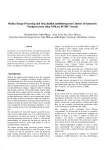
Like B-splines, the nonnegative basis functions of simplex spline volume sum to unity. They have a number of nice properties, such as the convex hull property, local support, affine invariance. Shape design based on trivariate DMS-spline volume includes the specification of a domain tetrahedralization, knot sequences, and control points to generate an initial shape. The initial shape is then refined into the final desired shape through interactive adjustment of domain tetrahedralization, control points, and knots. The geometric flexibility of simplex spline volumes provides great power on its shape editing. Figure 1 show a cubic trivariate DMS-spline solid corresponding to a domain with a single tetrahedron. Note that our trivariate DMS volumes represent not only boundary geometry, but also interior solid geometry. They can represent physical or material attributes over the entire solid as well. Figure 1 shows scaled tetrahedra of the solid in order to emphasize its non-empty solid interior geometry. For a general trivariate DMS-spline volume, each domain tetrahedron I has its own set of control points cIβ . However, in this paper, we consider a more restricted class of volumes by sharing respective control points along common triangles of two adjacent tetrahedra in parametric tetrahedralization. Splines with shared control points have a direct visual effect in geometric and solid modeling. More importantly, as proved by Dahmen et. al [DMS92], a degree


geometry, a material (e.g., density) function over s(x) can be simultaneously defined as gIβ g (7) NβI (x), (x) = ∑ I s p β i

(a)

(b)

Figure 1: (a) A cubic trivariate DMS-spline solid corresponding to a single tetrahedral domain with 20 control points. (b) The tetrahedra of the designed solid object are scaled to show the interior of the solid.

n trivariate DMS-spline with shared control points can be evaluated with the efficiency of a degree n − 1 spline. s(u) =

∑ ∑

I∈Ω |β|=n−1

cˆ Iβ (u)NβI (u)

where g can be color, texture, mass, temperature, or other visual or material functions as stated above. Visual and material modeling is indispensable for computerized virtual environments. Besides commonly-used material distributions in classical mechanics, it can be generalized to heat transfer, electricity, and beyond. The diverse set of these novel solid models are unique and invaluable because they can potentially unify geometric, topological, kinematic, material, and dynamic properties. The field attributes can be modified by directly changing the control coefficients stored at the control points. In addition, by moving the control points, we can perform FFD of the underlying geometric space. As a result, this procedure deforms the field properties and provides an alternate interaction mechanism. The geometric space over which the field is defined can be of arbitrary topology, which adds further shape editing flexibility.

where cˆ Iβ (u) =

4. Multiresolution Modeling

3

∑ cIβ+e

m

λm (u|pi , q j , rk , sl )

m=0

and em = (δi,m )3i=0 , m = 0, 1, 2 as the coordinate vectors. This property can significantly improve the software system for rendering a DMS-spline volume. It also implies that the knots {ti,n |i ∈ N} has no effect on the value of s(u). Note that for our trivariate DMS spline volumes, the used tetrahedral domain is not necessary to undergo a separate parameterization process, because it is already conforming to the three-dimensional physical domain for material attributes. The generalized control vectors are now (n + 3) vectors, including control points (px , py , pz ) for the solid geometry, and control coefficients (g1 , · · · , gn ) for the attributes, where n denotes the number of attributes associated with the geometry. 3.3. Coupling Solid Geometry and Physical Attributes In our framework, we consider a control coefficient (and possibly other vector-based quantities with n components) is associated with a corresponding control point and evaluated with the geometry simultaneously based on the same tetrahedral domain. In this way, we shall generalize DMS spline technique from geometric domains to visual or material domains. Typical material-oriented examples include: mass, damping, stiffness (such as strain and stress), and displacement for solid physics; or density, velocity, and pressure for fluid mechanics, etc. These attributes may be assigned at the control points or fitted by using both control vectors and knots. Other commonly-used visual information include: color, texture, intensity, opacity, transparency, etc. This flexibility permits our paradigm to be employed in a wide variety of applications involving continuous domains, such as finite element analysis, virtual sculpting, and computational fluid simulation. Consider that control coefficients gIβ are associated with control

points pIβ (gIβ may be a multi-dimensional vector). Besides solid

Based on the flexible simplex splines, we can easily achieve multiresolution modeling of heterogeneous solid objects. The multiresolution capability is achieved by interactively subdividing any region of interest and allocating more knots and control vectors accordingly. 4.1. Interactive Tetrahedralization We use Delaunay tetrahedralization to construct a tetrahedral domain, which serves as the tetrahedral domain of the trivariate simplex spline. In fact, the scalar simplex splines lend itself well appropriate for an unstructured grid volume representation. For constructing Delaunay tetrahedralization for a 3D point set, we make use of the incremental flip algorithm proposed in [Joe91, ES92]. The procedure to update a tetrahedralization is to insert one new vertex at each step. Then, a sequence of actions are applied to modify the tetrahedralization locally. Each flip action consists of replacing one, two, or three adjacent tetrahedra with four, three, or two new tetrahedra, respectively. When the new vertex lies either on a triangular face or on an edge of the current tetrahedralization, other face flips may be needed. When performing Delaunay tetrahedralization, the user have an option to enforce the quality constraints (including volume of tetrahedron, etc.). The user can also interactively specify boundary constraints (such as points, edges, polygons, or cells). We implement the boundary conforming Delaunay tetrahedralization [She97], which tries to recover the missing boundary edges of the piecewise linear complexes from its current Delaunay tetrahedralization by inserting new points. 4.2. Geometric Editing Using Control Points With this flexible modeling technique, we can easily design solid geometric shapes with sharp features and associated high frequency material properties. Since the control vectors include the position c The Eurographics Association 2004.


of control points and associated control coefficients, editing of control points and/or control coefficients offer more powerful modeling capabilities. Based on our experiments, we observe that associating control points to a domain in such a way: locating control points at the edges of tetrahedra of the domain, can well preserve the shape and features represented by the original domain. The difference between the geometry of the domain and the resulting DMS solid object is very small.

its quality conforming Delaunay mesh. Badly shaped elements from the mesh are eliminated and replaced with well shaped ones. This is done by automatically inserting additional points into current mesh. From Figure 4(b), we can see that more knots are generated around feature edges. By associating control points with the defined domain, all the features are preserved in the resulting DMS solid of degree 4. Please refer to Figure 4(d).

Moving control points around can lead to a desired deformation of the underlying model easily. Figure 2 shows an example. Figure 2(a) shows the domain of the cubic DMS solid, which is a torus. The user moves the control points to the new locations as shown in the solid mesh in Figure 2(b). Six very sharp corners are formed on the original solid object.

(a)

(b)

Figure 2: (a) The domain is a torus. (b) The deformation of the object is achieved by moving the control points to the new locations. The mesh shows a part of control nets, while the flat shaded surface indicates the resulting solid objects. Usually when the number of control points is very large, it is tedious and relatively difficult to manipulate the control points individually. In our system we provide Free-Form Deformation (FFD) tools to allow users to move control points. Figure 3 shows another example, where the domain is 5 separated tori as shown in Figure 3(a), and the DMS solid is quadratic. After the initial control points are generated, the user employ the bending FFD tool to relocate the control points to achieve the design shown in Figure 3(b). Note that, it is almost impossible for B-splines to model such objects whose domain is of non-trivial topology.

(a)

(b)

Figure 3: (a) The domain consists of 5 separated tori, which is of non-trivial topology. (b) The deformation of the object is achieved by bending the control net.

(a)

(b)

(c)

(d)

Figure 4: (a) The piecewise linear boundary constraints that the user specifies. (b) The multiresolution tetrahedralization conforming to the piecewise linear boundary constraints. (c) The color map of material distribution of the designed object. (d) Volume rendering of the designed object, where we can see that all the geometric shape features are preserved.

4.3. Attribute Editing Using Control Coefficients or Control Points Besides modeling solid geometry, the user can easily edit associated physical or material attributes as well. This is achieved by editing control coefficients at the corresponding control points, because the underlying material distribution is in fact a trivariate simplex spline defined over the same tetrahedralization. In the most simple form, the (multi-dimensional) control coefficients can be in one-to-one correspondence to their control-point counterparts which are used to define arbitrarily curved solid geometry over the same parametric domain (which is the initial tetrahedralization). However, local refinements for material modeling are frequently desirable in order to represent high-frequency features in the material domain. Our system allows users to interactively sketch skeletons. Each skeletal element is then associated with a locally defined implicit function; individual functions are blended using a polynomial weighting function that can be controlled by the user. After specifying these, the scalar control coefficients of the DMS-spline solid are assigned as the evaluations of the blending of field functions gi of a set of skeletons si (i = 1, · · · , N) at the positions of corresponding control points, f (x, y, z) =

N

∑ gi (x, y, z),

(8)

i=1

Figure 4 shows another example. The user first builds a 3D piecewise linear complex as shown in Figure 4, then our system generates c The Eurographics Association 2004.

where the skeletons si can be any geometric primitive admitting a well defined distance function: points, curves, parametric surfaces,


simple volumes, etc. The field functions gi are decreasing functions of the distance to the associated skeleton, gi (x, y, z) = Gi (d(x, y, z, si )),

(9)

where d(x, y, z, si ) is the distance between (x, y, z) and si , and Gi can be defined by pieces of polynomials or by more sophisticated anisotropic functions. Therefore, the user may enforce global and local control of an underlying scalar field in three separate ways: (1) defining or manipulating of the skeleton, (2) defining or adjusting those implicit functions defined for each skeletal element, and (3) defining a blending function to weight the individual implicit functions.

(a)

(b)

(c)

(d)

Figure 4 shows an example, where the user uses a mouse to freely sketch a curve inside the engineering part and defines an implicit 1 function, f (d) = 1+d 2 , to associate with the skeleton. Then the scalar control coefficients at the control points are assigned according to the skeleton function. The resulting material distribution is shown in Figure 4(c)(d). As shown in Figure 5, the user sketches a solid modeling conference logo, “SM”, with free hand inside a domain, which is a torus. After associating control points with the torus domain and assigning control coefficients according to the distance function to the sketched curve logo, the resulting geometry and its associated scalar field can be easily generated. In this example, we use a trivariate DMS-spline of degree 4. Figure 5(a) shows the volume rendering of the entire object. We can clearly see the resulting geometry and its associated attribute field. In Figure 5(b), the shaded surface shows the isosurface of the attribute field of the solid torus, which is generated using Marching Tetrahedra Method that we developed (We will discuss it in Section 6.2).

Figure 6: (a) Define a skeleton inside the Stanford bunny model for material editing. (b) The generated tetrahedral mesh of the Stanford bunny model. (c) Direct volume rendering of the resulting attribute field over the bunny model. (d) The color map of one slice of the bunny model shows the resulting attribute distribution.

By aligning free knots along the feature lines/faces in the domain, sharp features in both geometric and attribute fields can be modeled. As we state in Section 4.2, associating control points to the edges of tetrahedra of a domain can also well preserve the shape and features represented by the original domain. Let us see Figure 4 as an example. All the geometric features shown in the original domain are well preserved in the final resulting geometric object as shown in Figure 4(d).

(a)

(b)

Figure 5: (a) Editing attributes inside the tetrahedral domain of the torus model. From the direct volume rendering, we can clearly see the geometric boundary of the torus and the highlighted attributes. (b) Marching tetrahedra rendering of an isosurface of the resulting attribute field over the torus model. The greyscale background shows the torus geometry.

In Figure 6, the user is trying to design a digest system of the bunny model. The user draws a ellipsoid like shape to represent its stomach and two pipes adjacent to it (Illustrated in Figure 6(a)). Figure 6(b) shows the tetrahedralization of the bunny, which serves as the domain. In this example, we use a quadratic trivariate DMSspline. After associating control points with the domain, the resulting geometry and its associated attribute field can be easily generated. Please see Figure 6(c)(d).

In addition, by moving the control points, we can perform FFD of the underlying geometric object. As a result, this procedure deforms the associated attribute field. This is an alternate interaction mechanism for editing attributes. 5. Feature Sensitive Data Fitting To model data or attribute over the simplex spline based volume, it is much more desirable to have a fitting tool in addition to modeling tools as presented above. In this section, we propose a feature sensitive data fitting algorithm. That means the fitting algorithm can represent the data over the volume accurately and recover all the features with as few control vectors and bases as possible. Also the geometry of the volume is recovered simultaneously. Note that in the following section, we mainly discuss how to fit an unstructured volume. In fact, it can be any format, consisting of a set of points with associated attributes (i.e., (x, y, z, d1 , · · · , dn )). Figure 7 shows the spx model from the fluid dynamics research community. In order better to show the advantages of our fitting algorithm. We upsample the spx dataset from 2896 sampling points to 15832 points. c The Eurographics Association 2004.


points is finite. The number of tetrahedra needed for fitting at the desired accuracy depends on the user-specified error bound and the datasets. 5.2. Finding a Good Initial Tetrahedralization

Figure 7: (a) The point view of the spx dataset, where the color indicates the density difference. (b) Volume rendering of the spx dataset.

5.1. The Fitting Algorithm The problem of fitting volume data can be stated as follows: given 4 a set P = {pi }m i=1 of points pi = (xi , yi , zi , di ) ∈ R , find a trivariate 3 4 DMS volume s : R → R that approximates P. Unlike the existing fitting algorithms with parametric representations which usually find a one-to-one mapping between the data points and the points in the parametric space, our method skips this parameterization procedure. As stated before, we first build up a tetrahedralization parametric domain which is close to the original geometry of the tobe-fitted dataset. This domain serves for fitting both geometry and attributes. We use the position (xi , yi , zi ) of the data point pi as its parametric value. Therefore, we need to minimize the following objective function: min E =

m

∑ (pi − s(xi , yi , zi ))2 .

(10)

i=1

Our fitting algorithm treats both control vectors and knots as free variables. In this way, it can greatly reduce the approximation error given the same number of control vectors and knots. The tight coupling of both geometry and attributes during data fitting enables further editing on the continuous representation by means of moving control points, FFD, or changing control coefficients as we discussed in the Section 4, even after the fitting process is done.

As we can see from the fitting algorithm, a good initial basis will save a lot of time of performing recursive refinement and local fitting. More important, it can help to preserve geometric features of the original volume datasets. Essentially, there should be more primary knots distributed in the region containing features. Therefore, the dataset will undergo a preprocessing stage before fitting. First we have to find the proper tetrahedralization of the point sets. We perform the Delaunay tetrahedralization of the point set. Now we have to consider how to remove those tetrahedra which are outside the actual object. We place a ball at every point, whose radius is equal to the shortest distance from this point to its one-ring neighbors. Then, we perform the union of balls to obtain an occupancy map, which can roughly indicates the boundary of the actual object. Figure 8(a) illustrates the occupancy map of the point set of the spx dataset. Third, we check each tetrahedron to see if all the center points of its six edges are inside this occupancy map. If not, this tetrahedron is clipped away. Figure 8(b) shows the occupancy map and the Delaunay tetrahedralization together, where we can see some of tetrahedra are outside the occupancy map. From Figure 8(c), we can see that all the outside tetrahedra are removed and the final tetrahedralization of the point set is obtained. In this paper, we consider the fact that the real datasets to be fitted are usually densely sampled. This algorithm does not work well for very scattered datasets. Note that, this preprocessing is to produce a tetrahedral domain, not to generate the tetrahedralization of the object. The domain tetrahedralization should be much coarser than the tetrahedralization of the object as shown in Figure 8(c).

We first give an overview of our fitting algorithm. Then we will discuss some related issues in detail. 1. Create a tetrahedral domain for the entire volume domain, which fully contains the fitted volumetric object; 2. Solve Equation 10 by treating control vectors as free variables. 3. for each node ti of the tetrahedralization, if the fitting error in its 1-ring neighboring tetrahedra is larger than a user-specified value, solve Equation 10 by treating the knots associated to ti as free variables. 4. For each tetrahedron, if its fitting error is larger than a threshold ε, then subdivide it into four tetrahedra and repeat (2-4) until the fitting error of every tetrahedron is less than ε This algorithm will not stop until the fitting error in each tetrahedron is less than the user-specified error bound. Then the discrete point set with the associated attribute field is converted to a continuous spline-based volumetric implicit function, which can be evaluated at arbitrary sampling resolution and rendered with the direct volume rendering or the Marching Tetrahedra algorithm. The fitting algorithm is guaranteed to converge since the number of sampling c The Eurographics Association 2004.

(a)

(b)

(c)

Figure 8: (a) Occupance map of the point set. (b) The Delaunay tetrahedralization of the point set. (c) The final tetrahedralization after removing the outside tetrahedra. In order to let the generated tetrahedral domain faithfully reflect the nature of the object, the features should be considered in tetrahedralization. Essentially, we have two types of features since we consider both the geometry and physical attributes. Geometric features are one category and field features belongs to another category. Geometric features mean those regions where C 0 continuity occurs. We use an efficient algorithm to classify the boundary vertices. The boundary vertices are identified as corner vertex, curve vertex, and general boundary vertex. The classification algorithm is based on the solid angle at each vertex. The solid angle αi of


tetrahedron I(p0 , p1 , p2 , p3 ) at vertex p0 is defined to be the surface area formed by projecting each point on the face not containing p0 to a unit sphere centered at p0 . An equation for the computation of solid angle αi is given by Liu et al.[LJ94]: sin α2i = 12v/ ∏1≤i< j 0, using the linear decomposition, we can obtain: Z L 0

M(u(t)|V)dt =

Z L 3

∑ λ(xc + tdc )M(xc + tdc |V \ {xk })dt

0 j=0

n

0

Z L 0

M(xc + tdc |V)dt

M(xc + tdc |V)dt.

(15)

Replacing Equation 15 in Equation 13, we can obtain the following equation: Z L 0

M(xc +tdc |V)dt =

n n+1

3

Z L

j=0

0

∑ λ(xc )

M(xc +tdc |V\{xk j })dt. (16)

When n = 0,

Z L 0

M(xc + tdc |V)dt =

L . Vol(V)

With the above equation, we can efficiently evaluate the integral of densities along a casted line. Besides the X-ray volume rendering, we can also perform general ray casting. Since the solid object is represented by a single trivariate DMS-spline, our ray casting avoids resampling and interpolation problems.

gIβ NβI (u(t))dt)

Z L

= −

Z 1 L

1 n

j

6.2. Marching Tetrahedra Isosurfacing Since the resulting heterogeneous solid object consists of tetrahedra, it is easy to perform marching tetrahedra isosurfacing to extract an isosurface of its associated field. Please refer to [CDM∗ 94] for the detail of a marching tetrahedra algorithm. It is important to note that, based on the geometry of the primary knots, the samples may be spaced at non-unit intervals or distributed very irregularly. Our approach does not require resampling onto a regular voxel raster, which would introduce error. Furthermore, along tetrahedron edges, the process of isosurface extraction employs the original trivariate DMS-spline interpolation, which has the potential to avoid introducing sampling artifacts. Since traditional voxel-based sculpting systems employ trilinear interpolation, they exhibit aliasing when the voxel grid is scaled or deformed. Aliasing must then be eliminated by filtering most or all of the voxel grid. We avoid this problem by using what is essentially a higher-order C n−1 trivariate spline. If the objects modeled by our approach are originally smooth, they will remain smooth even if the control lattice is arbitrarily scaled or even deformed. If they contain C 0 or discontinuity region, these features will be preserved as well. A key aspect of isosurface extraction is normal vector computation. With our polynomial-based approach, it can be determined c The Eurographics Association 2004.


Model

data pts

domain tetra

control pts

knots

geometric fitting error

field fitting error

spx

15832

1914

3335

992

8.21121 × 10−7

7.78170 × 10−4

cubecross

24128

2245

3294

858

1.25994 × 10−6

1.97281 × 10−4

router

34744

2812

4239

1236

1.13400 × 10−6

1.52832 × 10−4

Table 1: Statistics of Data fitting.

analytically. Furthermore, the local evaluation can lead to multiresolution isosurface extraction. When a tetrahedron of the object is determined cross the isosurface of its associated field, and its size is larger than a specified threshold, we can evaluate the trivariate DMS-spline and upsample it locally to increase the resolution and then perform isosurfacing on those smaller cells. Please see the illustration in Figure 13.

else some locations of the geometric object may not have attribute properties, or attribute properties are assigned to the locations outside the geometric object. When using the decoupling scheme, it is possible to model any number of attribute properties over the geometric object. Complicated geometries with simple attributes, and vice versa, may be represented at the resolution that best suits them. The gain may be a large savings in storage and execution time. Furthermore, noise is an important variable in any visualization involving measured data. Simplex splines generally provide a robust representation for a signal containing moderate noise. Compared with polygons, or higher dimensional analogues such as voxels, simplex splines generally represent a smooth function with fewer points. However, with our knots manipulation technique they can represent higher frequency features as well. 8. Conclusion

(a)

(b)

Figure 13: (a) The single tetrahedron in the solid object is larger than the specified size and is needed to be upsampled. (b) Based on the corresponding domain tetrahedron (as shown in mesh), the tetrahedron in the solid object is upsampled. Each cell is scaled a little in order to clearly observe the upsampling result.

7. Implementation and Discussion We have implemented a prototype system on a PC with 3.0 GHz P4 CPU and 2GB of RAM. The system is written in C++ and OpenGL. In our system we incorporate the Phantom 1.0 device from Sensable Technologies into our user interface. Users can use a mouse or the Phantom to manipulate the control points or sketch the skeletons. Table 1 shows the statistics of the performance of our fitting algorithm on several datasets, where the fitting error is the mean square error. As one can see, we couple geometric and attribute representation together in order to provide a unified paradigm to explicitly model geometry, topology, and its associated attribute properties. However, one weak point of this representation is that if the geometric features and attribute field features are not conforming to each other, we have to select the higher resolution to model both, even though it might not necessary for one of them to have such a high resolution. A potential solution for this case is to decouple geometric and attribute representations. Thus, it offers more flexibility to construct different resolution of tetrahedralization of a domain to fit the geometry and attribute distribution, respectively. But special care of aligning the boundaries of two domains exactly the same must be taken, or c The Eurographics Association 2004.

In this paper we have articulated a new integral approach for representing, modeling, reconstructing, and visualizing multidimensional, physical attributes across any volumetric objects. In particular, we employ a trivariate simplex spline model that is defined over a tetrahedral decomposition of any 3D domain. The modeled volume can be of complicated geometry and arbitrary topology. The trivariate simplex spline model ideally serves the pressing needs of both visualization and modeling communities since the model makes use of a more general and flexible tetrahedral domain and offers a compact continuous representation at the same time. More importantly, it integrates geometry and attribute properties over domains of arbitrary topology, by modeling a complicated heterogeneous object with a single trivariate simplex spline without any additional operations of trimming or patching. All of the above attractive characteristics result from many appealing properties of trivariate simplex splines such as piecewise polynomials of low degree, high-order continuity, and sharp feature modeling through different knot placements. In addition, we have developed a feature-sensitive fitting algorithm that can reconstruct a more compact trivariate simplex spline from a structured or unstructured volume. It reconstructs the geometry and the associated material attributes simultaneously, satisfying various continuity requirements set by the user. Such flexibility allows us to model continuous or discontinuous material distribution with ease. Our new representation can also facilitate multiresolution, local adaptive subdivision, free-form deformation, both isosurface and volume rendering, as well as other modeling and visualization functionalities. This is mainly because many of its nice analytical properties and associated computational tools. Based on our extensive experiments on using the trivariate simplex spline, we believe that our new paradigm can significantly advance the current state of the


knowledge in modeling and visualizing heterogeneous models of physical objects and their material properties. Besides solid modeling and volume visualization, in the near future we are pursuing other application directions including general data modeling, material editing and reconstruction, geometric processing of bio-medical and geological datasets, dynamic simulation and analysis of multiresolution, heterogeneous objects, etc.

[MC01]

M ARTIN W., C OHEN E.: Representation and extraction of volumetric attributes using trivariate splines: A mathematical framework. In Proceedings of the 7th ACM Symposium on Solid Modeling and Applications (2001), pp. 234–240.

[PS94]

P FEIFLE R., S EIDEL H.-P.: Faster evaluation of quadratic bivariate dms spline surfaces. In Proceedings of Graphics Interface ’94 (1994), pp. 182–189.

References

[PS95]

P FEIFLE R., S EIDEL H.-P.: Fitting triangular B-splines to functional scattered data. In Proceedings of Graphics Interface ’95 (1995), pp. 80–88.

[QT96]

Q IN H., T ERZOPOULOS D.: D-NURBS: A physicsbased framework for geometric design. IEEE Trans. on Visualization and Computer Graphics 2, 1 (1996), 85–96.

[QT97]

Q IN H., T ERZOPOULOS D.: Triangular NURBS and their dynamic generalizations. Computer Aided Geometric Design 14, 4 (1997), 325–347.

[RE99]

R AVIV A., E LBER G.: Three dimensioinal freeform sculpting via zero sets of scalar trivariate functions. In Proceedings of 5th ACM Symposium on Solid Modeling and Applications (1999), pp. 246–257.

[CCM∗ 00] C IGNONI P., C ONSTANZA D., M ONTANI C., ROC CHINI C., S COPIGNO R.: Simplification of tetrahedral meshes with accurate error evaluation. In Proceedings of the conference on Visualization ’00 (2000), pp. 85– 92. [CDM∗ 94] C IGNONI P., D E F LORIANI L., M ONTANI C., P UPPO E., S COPIGNO R.: Multiresolution modeling and visualization of volume data based on simplicial complexes. In Proceedings of the 1994 symposium on Volume visualization (1994), pp. 19–26. [dB76]

B OOR C.: Splines as linear combinations of Bsplines. In Approximation Theory II (1976), Academic Press, New York, pp. 1–47.

[DMS92]

DAHMEN W., M ICCHELLI C. A., S EIDEL H.-P.: Blossoming begets B-spline bases buit better by bpatches. Mathematics of Computation 59, 199 (1992), 97–115.

[RE01]

R AVIV A., E LBER G.: Interactive direct rendering of trivariate B-spline scalar functions. IEEE Transactions on Visualization and Computer Graphics 7, 2 (2001), 109–119.

[ES92]

E DELSBRUNNER H., S HAH N. R.: Incremental topological flipping works for regular triangulations. In Proceedings of 8th Annual ACM Symposium on Computational Geometry (1992), pp. 43–52.

[RN00]

[GS94]

G REINER G., S EIDEL H. P.: Modeling with triangular B-splines. IEEE Computer Graphics and Applications 14, 2 (1994), 56–60.

ROXBOROUGH T., N IELSON G. M.: Tetrahedron based, least squares, progressive volume models with application to freehand ultrasound data. In Proceedings of the conference on Visualization ’00 (2000), pp. 93– 100.

[She97]

H ONG W., K AUFMAN A.: Feature preserved volume simplification. In Proceedings of the Eighth ACM Symposium on Solid Modeling and Applications (2003), pp. 328–333.

S HEWCHUK J. R.: Delaunay Refinement Mesh Generation. PhD thesis, School of Computer Science, Carnegie Mellon University, 1997.

[SPS01]

H UA J., Q IN H.: Haptic sculpting of volumetric implicit functions. In Proceedings of 9th Pacific Conference on Computer Graphics and Applications (2001), pp. 254–264.

S CHMITT B., PASKO A., S CHLICK C.: Constructive modeling of frep solids using spline volumes. In Proceedings of the 6th ACM symposium on Solid modeling and applications (2001), pp. 321–322.

[SV94]

S EIDEL H.-P., V ERMEULEN A. H.: Simplex splines support surprisingly strong symmetric structures and subdivision. In Curves and Surfaces II. AK Peters, 1994, pp. 443–455.

[THJ99]

T ROTTS I. J., H AMANN B., J OY K. I.: Simplification of tetrahedral meshes with error bounds. IEEE Trans. on Visualization and Computer Graphics 5, 3 (1999), 224–237.

[YT00]

YAO J., TAYLOR R. H.: Tetrahedral mesh modeling of density data for anatomical atlases and intensitybased registration. In Proceedings of the third International Conference on Medical Image Computing and Computer-Assisted Intervention (2000), pp. 531–540.

[HK03]

[HQ01]

[HQ02]

[HQ04]

DE

H UA J., Q IN H.: Haptics-based volumetric modeling using dynamic spline-based implicit functions. In Proceedings of IEEE Symposium on Volume Visualization and Graphics (2002), pp. 55–64. H E Y., Q IN H.: Surface reconstruction with triangular B-splines. In Proceedings of Geometric Modeling and Processing, (2004).

[Joe91]

J OE B.: Construction of three-dimensional triangulations using local transformations. Computer Aided Geometric Design 8 (1991), 123–142.

[LJ94]

L IU A., J OE B.: Relationship between tetrahedron shape measures. BIT 34, 2 (1994), 268–287. c The Eurographics Association 2004.