Multirobot Object Localization: A Fuzzy Fusion Approach - AASS

IEEE TRANSACTIONS ON SYSTEMS, MAN, AND CYBERNETICS—PART B: CYBERNETICS

2

Multirobot Object Localization: A Fuzzy Fusion Approach

3

Kevin LeBlanc and Alessandro Saffiotti, Senior Member, IEEE

1

4 5 6 7 8 9 10 11 12 13 14 15 16

Abstract—In this paper, we address the problem of fusing information about object positions in multirobot systems. Our approach is novel in two main respects. First, it addresses the multirobot object localization problem using fuzzy logic. It uses fuzzy sets to represent uncertain position information and fuzzy intersection to fuse this information. The result of this fusion is a consensus among sources, as opposed to the compromise achieved by many other approaches. Second, our method fully propagates self-localization uncertainty to object-position estimates. We evaluate our method using systematic experiments, which describe an input-error landscape for the performance of our approach. This landscape characterizes how well our method performs when faced with various types and amounts of input errors.

17 Index Terms—Fuzzy logic, information fusion, multirobot 18 systems, object localization.

I. I NTRODUCTION

19 20 21 22 23 24 25 26 27 28 29 30 31 32 33 34 35 36 37 38 39 40 41 42

O

NE of the most important challenges in autonomous robotics is to accurately determine the state of the world. This knowledge is crucial to a robot’s ability to appropriately and reliably perform actions. In particular, it is important for a robot to know the positions of objects relevant to its current task. In this paper, we address the problem of determining this information in a multirobot system. The multirobot object localization problem can be seen as an instance of the more general information fusion problem. Combining information from different sources and/or different times, if done properly, yields more accurate estimates about the state of the world. In general, redundant information can improve accuracy and reliability, whereas complementary information can resolve ambiguities and incompleteness. In single-robot object localization, information about object positions arrives at different times and/or from different sensors. In multirobot systems, more sensors are available, often with different points of view and different characteristics. This can virtually extend the overall system’s field of view, as well as reduce the effects of sensor range and accuracy limitations. The advantages of multirobot systems come at a cost. Unreliable communication channels and bandwidth limitations can make it difficult to share information. Furthermore,

Manuscript received March 19, 2008; revised November 9, 2008. This work was supported in part by the National Graduate School in Computer Science (CUGS), Sweden. This paper was recommended by Associate Editor I. Bloch. The authors are with the Center for Applied Autonomous Sensor Systems, Department of Technology, Örebro University, 70182 Örebro, Sweden. Color versions of one or more of the figures in this paper are available online at http://ieeexplore.ieee.org. Digital Object Identifier 10.1109/TSMCB.2009.2015279

1

shared information must be represented in a common reference 43 frame—normally, a global coordinate system. Object-position 44 estimates in this frame will strongly depend on a robot’s knowl- 45 edge about its own pose in the frame. 46 This paper, which extends the work in [1], makes three 47 main contributions. First, we propose a fuzzy-logic-based ap- 48 proach to representing and fusing object-position information 49 in multirobot systems. Our method uses fuzzy sets to represent 50 information, and we perform fusion using fuzzy intersection. 51 This yields a consensus about the fused information, as op- 52 posed to the compromise produced by many other approaches. 53 Fuzzy logic has successfully been used in many areas of 54 robotics [2], including information fusion (e.g., [3] and [4]) and 55 self-localization (e.g., [5] and [6]); however, the use of fuzzy 56 logic to address multirobot object localization is new. Sec- 57 ond, our method fully considers uncertainty in self-localization 58 when converting local position estimates to global coordinates. 59 As we discuss in Section II, most existing approaches as- 60 sume perfect self-localization, which is often not achievable 61 in robotic systems. Finally, we suggest a methodology for 62 systematically evaluating our approach, where we characterize 63 its performance with respect to various types of errors on its 64 inputs. This analysis departs from the traditional approach to 65 evaluating subsystems in robotics, where tests are performed 66 only under typical conditions, and the subsystem under test 67 is specifically tuned for those conditions. Our methodology 68 allows us to see how a subsystem performs outside of its 69 comfort zone; this can be useful when deciding what method 70 to use for a given application. In addition to these contribu- 71 tions, we also present some approximations of our method, 72 which reduce computational and bandwidth requirements if 73 needed. 74 Often, fusion is combined with data association and pre- 75 diction to perform tracking. In this paper, we focus only on 76 the fusion process itself. To allow the performance of our 77 fusion method to be measured in isolation, we assume that 78 the identity of detected objects is known (which trivializes 79 data association), and we assume that objects are static (hence, 80 prediction is not needed). 81 The rest of this paper is organized as follows. In Section II, 82 we discuss related work. Section III gives a brief overview of 83 fuzzy sets and discusses how we use them to represent and 84 fuse uncertain position information. In Section IV, we describe 85 our overall framework for multirobot object localization, and in 86 Section V, we discuss our implementation of the framework. 87 Finally, in Section VI, we present and discuss the results of our 88 experiments; we conclude with Section VII. 89

1083-4419/$25.00 © 2009 IEEE

2

90


II. R ELATED W ORK

Object localization is a fundamental challenge in robotics, and as such, many works address it. However, most methods 93 rely on a relatively small number of underlying information 94 fusion approaches. In this section, we give an overview of the 95 fusion approaches that are most commonly used for object lo96 calization tasks in robotics. We also briefly discuss two related 97 problems—the self-localization problem and the multisensor 98 multitarget tracking problem. 99 Single-robot and multirobot approaches to object localization 100 are often addressed using the same underlying fusion tech101 niques. The main difference is that, in multirobot systems, 102 sensors usually have unknown relative positions, which means 103 that a common reference frame for position information is 104 needed. This reference frame is normally a global coordinate 105 system; such a reference frame is often used in other parts 106 of the overall system as well. Estimating object positions in 107 a global coordinate system normally requires that a robot 108 should know its own pose in this frame, i.e., self-localization 109 needs to be addressed. There are, however, a few approaches 110 that avoid the need for global self-localization by using rela111 tive reference frames, for instance, [7] and [8]. Once object112 position estimates have been situated in the common reference 113 frame—a step that is normally nontrivial given self-localization 114 uncertainty—single-robot and multirobot object localization 115 problems can be addressed using similar methods. 116 Many works address the self-localization problem (e.g., [5], 117 [6], [9], and [10]), and it is often combined with the mapping 118 problem (a survey of this field is presented in [11]). The 119 self-localization problem has some aspects in common with 120 the multirobot object localization problem, and similar fusion 121 methods are often used in both problems. However, a number of 122 different challenges are involved when dealing with multirobot 123 object localization. As such, we will only briefly touch upon the 124 self-localization problem when we discuss the landmark-based 125 fuzzy self-localization approach we use in this paper, which 126 is based on [5]. A similar approach is described in [6]; this 127 approach, which is also based on fuzzy logic, uses sonar scans 128 instead of landmarks to determine possible robot poses. 129 Fuzzy logic is a popular tool for addressing information 130 fusion problems [1], [3], [4]. For instance, [4] presents a 131 general approach to information fusion using fuzzy logic. This 132 general fusion approach is then applied to the single-robot 133 self-localization problem as an example. The work presented 134 here has similar foundations, both in terms of information 135 representation [2] and information fusion. This paper aims to 136 apply well-studied fuzzy information fusion techniques to the 137 multirobot object localization problem. As we will show, such 138 an approach has a number of built-in advantages. 139 Despite the popularity of fuzzy logic for addressing informa140 tion fusion in general, many robotics applications rely on proba141 bilistic fusion techniques. A large number of object localization 142 methods are based on Kalman filters [12], [13] and linearized 143 Kalman filters, like the extended Kalman filter [14], [15] and 144 the unscented Kalman filter [16]. The Kalman filter algorithm 145 can be seen as a continuous-space implementation of the Bayes 146 filter algorithm [17], [18], in which information is represented 91

92

using Gaussians. In general, such methods are accurate, easy to 147 implement, and computationally efficient. They are used both 148 to fuse information arriving at different times and to combine 149 information arriving from different sources (e.g., [19]–[23]). 150 Despite their widespread use, Kalman filters have a number of 151 limitations. For one thing, they are unimodal. This limitation 152 can be somewhat offset by multiple hypothesis tracking [24], 153 [25], which allows multiple modes to be maintained in paral- 154 lel. Another limitation of Kalman filter-based methods is that 155 since information is combined using weighted averaging, fused 156 results can significantly be degraded in the presence of false 157 positives or outliers. Various forms of gating (e.g., [26]–[28]) 158 can be used to reduce the effects of this limitation; however, 159 this requires careful tuning. 160 Markov localization (e.g., [10] and [29]) is another prob- 161 abilistic method often used in robotic localization tasks. The 162 algorithm can be viewed as a discrete-space implementation 163 of the Bayes filter algorithm [18]. The idea is to maintain 164 a (possibly multimodal) discrete probability distribution over 165 the state space—this is normally either grid-based or sample- 166 based. New information increases the probability that an ob- 167 ject is in a given region of the distribution and decreases 168 the probability that it is anywhere else. The resulting distri- 169 bution will typically have a higher probability in positions 170 that are consistent with the majority of the fused information. 171 Markov localization has been shown to be robust, although it 172 is computationally more demanding than Kalman filtering, in 173 general. There is typically a tradeoff between accuracy and 174 computational load; sample-based methods, in particular, allow 175 a smooth transition along the axis of this tradeoff. A hybrid 176 method that combines Kalman filters with Markov localization, 177 called Markov–Kalman object localization, has been shown to 178 be very effective [30], [31]. 179 The multisensor multitarget tracking problem is closely re- 180 lated to the multirobot object localization problem, except 181 for the fact that, in the former, sensors normally have fixed 182 positions. The vast majority of tracking approaches combine 183 observations using either Kalman filtering or sample-based 184 probabilistic filtering [22], [29], [32], [33]. Recent develop- 185 ments in this field mainly aim at improving performance with 186 respect to data association and prediction. Data association, 187 in particular, is known to be a computationally complex and 188 difficult problem, and many approaches focus on this; [34] 189 provides a survey of this field. Recall that, in this paper, we 190 do not address data association or prediction. 191 We have discussed the most common approaches to fusion in 192 multirobot object localization, all of which share one significant 193 limitation: self-localization uncertainty is not considered. Most 194 works explicitly assume perfect self-localization, which is not 195 normally achievable in robotic systems. In particular, even 196 small errors in orientation can cause large errors in object- 197 position estimates. 198 Aside from the work that we are extending [1], we know 199 of only one approach that explicitly addresses self-localization 200 uncertainty when performing multirobot object localization 201 [35]; in this sample-based approach, a small number of possible 202 object positions are computed taking self-localization uncer- 203 tainty into account, and these are exchanged between robots. 204

LEBLANC AND SAFFIOTTI: MULTIROBOT OBJECT LOCALIZATION: A FUZZY FUSION APPROACH

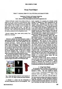
Fig. 1.

Various types of uncertainty represented using fuzzy sets. Figure from [2], used with permission.

214 215 216

In a few other approaches, self-localization uncertainty is used to weight estimates of target object positions (e.g., see the arithmetic mean method in [21]; a similar idea is described, but not implemented, in [19]). The work in [36] demonstrates that considering reliability of sources, in general, can improve performance in both self-localization and object-localization tasks. The method we propose uses fuzzy logic to compute a consensus between sources, and it does not suffer from the effects of averaging. Moreover, our method fully considers self-localization uncertainty when computing object-position estimates.

217

III. F UZZY P OSITION I NFORMATION

218 219

223

In this paper, we use fuzzy sets to represent and combine information about the positions of robots and objects. Fuzzy sets provide a powerful and convenient way to represent and fuse possibly uncertain position information. This section gives a brief overview of fuzzy sets, which should allow the reader to understand how they are used in this paper.

224

A. Representing Fuzzy Position Information

225 226

Fuzzy sets were proposed by Zadeh [37] as a way of representing noncrisp concepts (e.g., tall or old) by allowing set elements to have degrees of membership. These degrees of membership are represented by real numbers in the [0, 1] interval. Given an element x belonging to the universal set X, one can denote the degree of membership of the element x to the set described by the concept A as µA (x). Mathematically, membership functions are defined as

205 206 207 208 209 210 211 212 213

220 221 222

227 228 229 230 231 232

µA : X → [0, 1]. 233 234 235 236 237 238 239 240 241 242

3

(1)

In this paper, we adhere to a possibilistic interpretation of fuzzy sets [38], [39], where µA (x) indicates the degree of possibility that x possesses the property A. Therefore, if A represents the position of an object, we read µA (x) as “the degree of possibility that object A is at position x.” Note that under this interpretation, low possibility values actually provide more information than high values, as they rule out potential elements. In particular, complete ignorance is represented by a fuzzy set in which all elements have membership values of 1.0—in other words, all values are equally and fully possible.

Conversely, the most informative distributions are those in 243 which all elements have membership values of 0.0 except for 244 one, which has a membership value of 1.0. 245 The use of fuzzy sets allows us to represent several different 246 types of uncertainty in position information. The ability to 247 represent information at precisely the level of detail at which 248 it is available is often claimed to be one of the most compelling 249 reasons to use fuzzy sets. Fig. 1 illustrates some of these 250 uncertainty types. In Fig. 1(a), the position of the object is 251 known with certainty to be 80. In Fig. 1(b), the position is 252 approximately 80, and it is, therefore, vague. In Fig. 1(c), the 253 position is between 80 and 160, and it is, therefore, imprecise. 254 In Fig. 1(d), the position is either 80 or 160, and it is, therefore, 255 ambiguous. In Fig. 1(e), the position is, with the highest pos- 256 sibility, at 80, but it is also possible that it is elsewhere (e.g., 257 perhaps it has recently been seen at 80, but it might have been 258 moved since then)—this unreliability is represented by setting 259 a minimum value for all elements in the fuzzy set to a certain 260 bias value. Finally, in Fig. 1(f), there are a number of different 261 types of uncertainty combined. 262 Sometimes, it is useful to extract a point estimate Aˆ ∈ X 263 from the information contained in a fuzzy set µA . This process 264 is called defuzzification and can be done in a number of ways. 265 One of the most common defuzzification techniques is to use 266 the center of gravity (CoG) of the fuzzy set µA , which is 267 computed according to the following: 268 xµA (x)dx Aˆ = x∈X . (2) x∈X µA (x)dx B. Fusing Fuzzy Position Information

269

There are a number of operations that can be performed on 270 fuzzy sets; some of the most common are intersection, union, 271 and complementation. In this paper, we focus on intersection, 272 which can be used to fuse information represented in fuzzy sets. 273 Intersection of fuzzy sets is normally defined as 274 µA∩B (x) = µA (x) ⊗ µB (x)

(3)

where ⊗ denotes a triangular norm or t-norm [40]. T-norms 275 are binary operators that are commutative, associative, and 276 nondecreasing (if x ≤ y, then x ⊗ z ≤ y ⊗ z) and have 1 as 277 the neutral element (x ⊗ 1 = x). The most commonly used 278

4


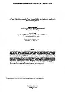
Fig. 2. (a) Fuzzy fusion computes a consensus between two sources of information, as opposed to (b) averaging approaches, which compute a tradeoff.

t-norms are the minimum, the product, and the Łukasiewicz operator max(x + y − 1, 0). The various t-norms behave differently; the choice is typically domain dependent. For instance, the minimum t-norm is 283 idempotent [min(x, x) = x]. Therefore, this operator is often 284 used when the independence of sources cannot be assumed. 285 This is because fusing the same information multiple times 286 using an idempotent operator yields the same result as fusing 287 it only once. Therefore, it does not matter if the sources are 288 dependent—which means they could be providing different 289 versions of the same information. 290 In this paper, we typically use the product t-norm, which 291 is nonidempotent. The product should be used when indepen292 dence is granted since it acts as a reinforcing operator; specifi293 cally, it reinforces belief in values that are deemed possible by 294 all sources. See, for example, [4] for more details. 295 As an example, imagine two sources that both report that 296 µA (x) = 0.5 and µA (y) = 1.0. Recall that under the interpre297 tation of fuzzy sets used here, µA (x) is the possibility that 298 element x has property A. If the sources are dependent, then 299 they are potentially merely repeating the same information. For 300 instance, the information might reflect the beliefs of two people 301 who have read about an event in the same newspaper. In this 302 case, the information should be combined using the idempotent 303 minimum t-norm, which will result in the combined belief 304 being the same as the inputs µA (x) = 0.5 and µA (y) = 1.0. 305 Since the sources are not independent, there is no reinforcement 306 effect, although the sources agree. 307 On the other hand, if the sources are independent, then they 308 are not merely repeating the same information. For instance, 309 the information might reflect the beliefs of two people who 310 have both witnessed an event. In this case, we can apply a 311 reinforcing t-norm, like the product, which will result in a 312 combined belief of µA (x) = 0.25 and µA (y) = 1.0. This belief 313 is stronger than any of the individual ones because it narrows 314 the set of possibilities more sharply. In this sense, the two 315 opinions have been reinforced. 316 There are two important general facts about fuzzy fusion that 317 should be noticed. First, only values that are regarded as possi318 ble by all sources are retained in the result. This can be seen in 319 the simple example shown in Fig. 2(a). In the figure, the result 320 of the fusion of fuzzy sets µ1 and µ2 using the minimum t-norm 321 is indicated by the shadowed area. Intuitively, the result of fuzzy 322 fusion represents a consensus between sources of information. 323 This contrasts with techniques that use averaging, which yield a 324 tradeoff. Fig. 2(b) shows how two items of information similar 325 to the ones shown in Fig. 2(a) might be represented and fused in 326 an averaging approach. Notice that with fuzzy fusion, the peak 279

280 281 282

Fig. 3. Discounting unreliable information in fuzzy fusion. Information µ1 is unreliable, as indicated by the high bias, and, therefore, only has a small influence on the result of the fusion.

of the resulting distribution coincides with the peak of µ2 since 327 this is compatible with the peak of µ1 ; it lies in between those 328 peaks when using averaging. 329 The second fact to note is that fuzzy fusion automatically dis- 330 counts unreliable information. Consider Fig. 3. The information 331 represented by µ1 includes a high bias (0.8), indicating that this 332 information is unreliable; the information represented by µ2 333 has a small bias (0.1). Correspondingly, the result of the fusion 334 (here using the product t-norm) is similar to the information in 335 µ2 , and it is only marginally influenced by µ1 . Fuzzy fusion 336 minimizes the impact of unreliable information, provided this 337 unreliability is correctly represented. 338 IV. O BJECT L OCALIZATION F RAMEWORK A. Problem Formulation

339 340

Our framework assumes that we have a set of M robots, 341 denoted {r1 , . . . , rM }, with M > 1, which are able to com- 342 municate in some way. We also assume that a global reference 343 frame for position information is available and known to all 344 robots. A robot’s knowledge about its own position in this 345 reference frame may be uncertain. This reference frame could 346 be dynamic; however, in this paper, we use a fixed global coor- 347 dinate system. Positions in the global frame are denoted (x, y), 348 and poses, which include orientation, are denoted (x, y, φ). 349 Each robot ri maintains a belief distribution about its own 350 pose in the world. We make no assumptions about how this 351 distribution is created or maintained; we simply require that, 352 at all times, each robot can determine, for any pose (x, y, φ), 353 how much it believes this to be its true pose. In practice, we 354 represent self-localization information as we represent other 355 types of position information: using a fuzzy set, which indicates 356 the possibility of a given pose being a robot’s true pose. 357 In Section V-B, we will briefly describe the landmark-based 358 approach to self-localization used in this paper. 359 We assume that robots can observe named objects in the 360 environment, and that the identity of an observed object is 361


Fig. 4.

Overall schema of our multirobot object localization method.

368 369

known. An observation includes an estimate of the object’s position relative to the robot, as well as some associated uncertainty (e.g., a sensor model). In this paper, we use range and bearing measurements to represent observations, denoted (ρ, θ), and we use separate sensor models for the range and bearing components. We do not consider the orientation of observed objects, although an extension of our framework to include this would be straightforward.

370

B. Overall Schema

371 372 373

The overall schema of our method for multirobot object localization is graphically represented in Fig. 4 for a case with two robots sharing information about one object. In general, there are five main items of position information that we need to represent in each robot i. Note that each of these is time varying; we omit the time indexes for simplicity. S i A 3-D fuzzy set representing robot i’s self-localization estimate, in global coordinates. For any pose (x, y, φ), S i (x, y, φ) measures robot i’s belief that it is at that pose. Lij A 2-D fuzzy set representing robot i’s local objectposition estimate for object j, in polar coordinates. For any (ρ, θ), Lij (ρ, θ) measures the possibility that object j is at distance ρ and bearing θ with respect to robot i. Note that single-point, range-only, and bearingonly estimates can all be represented in this fuzzy set. ˆ is represented by setting A single-point estimate (ˆ ρ, θ) ˆ = 1 and Li (ρ, θ) = 0 elsewhere. A bearing-only Lij (ˆ ρ, θ) j measurement of θˆ is obtained by setting Lij (ρ, θ) = 1 ˆ and 0 otherwise. A range-only measurement if θ = θ, of ρˆ is obtained by setting Lij (ρ, θ) = 1 if ρ = ρˆ, and 0 otherwise. Gij A 2-D fuzzy set representing robot i’s global objectposition estimate for object j, in global coordinates. For any position (x, y), Gij (x, y) measures the possibility that object j is at position (x, y). Fji A 2-D fuzzy set representing the fused object-position estimate maintained by robot i for object j, in global coordinates. For any position (x, y), Fji (x, y) measures the possibility that object j is at position (x, y), according to the fusion of robot i’s own global estimate with those available from other robots. Cji A single (x, y) position representing the crisp objectposition estimate maintained by robot i for object j, in global coordinates. This is extracted from Fji .

362 363 364 365 366 367

374 375 376 377 378 379 380 381 382 383 384 385 386 387 388 389 390 391 392 393 394 395 396 397 398 399 400 401 402 403 404 405

5

Our method consists of the following three main processing 406 steps, which operate on the described items of information. 407 These steps are individually carried out inside each robot. Note 408 that the descriptions below do not specify when each step 409 should be performed—this will be discussed in Section IV-E. 410 1) Coordinate Transformation: An observation of a target 411 object j is represented in a local estimate Lij , which reflects 412 the measured range and bearing, as well as the sensor models 413 for each of these. This estimate Lij is transformed into a global 414 estimate Gij via a fuzzy coordinate transformation, described 415 in Section IV-C. This transformation considers the full self- 416 localization distribution S i when computing Gij ; that is, all self- 417 localization uncertainty is propagated to Gij . This is one of the 418 main distinctive features of our method. 419 2) Multirobot Fusion: In this step, robot i combines its 420 global estimate Gij with those of other robots. The fusion of 421 fuzzy sets was briefly described previously. The details of the 422 fusion step are discussed in Section IV-D. The result of the 423 fusion is stored in Fji . 424 3) Position Extraction: When a point estimate of the posi- 425 tion of object j is needed by robot i, e.g., for action planning or 426 execution, it is extracted from the latest fused object estimate 427 Fji . This estimate Cji is computed by taking the CoG of Fji 428 according to (2). 429 Fig. 5 shows a graphical example of how the fuzzy sets 430 previously described might look after a few observations. The 431 fuzzy set in the top left corner for each robot is the self- 432 localization estimate S i ; the middle fuzzy set is the global 433 estimate Gij ; the rightmost fuzzy set is the fused estimate Fji . 434 The observation is shown in the bottom left corner. Note that 435 robot 1’s global estimate is not simply a translation of its self- 436 localization estimate; this is due to the uncertainty in both the 437 observation and the robot orientation. Also, note that robot 2 438 has much less uncertainty in self-localization; correspondingly, 439 the fused estimate, which is identical for both robots, is very 440 similar to robot 2’s global estimate. 441 Next, we will describe in detail the coordinate transformation 442 and multirobot fusion steps, which constitute the core steps of 443 our approach. After that, we will describe how the steps are put 444 together to form the overall framework. 445 C. Coordinate Transformation

446

The coordinate transformation step converts a local object- 447 position estimate Lij into a global object-position estimate Gij , 448 taking the self-localization estimate S i into consideration. Note 449

6


Fig. 5. Snapshot of our framework after a few observations, in a scenario with two robots. Lighter areas indicate possible positions; darker areas are less possible. We do not show the uncertainty in the range and bearing of the local estimates (bottom left for each robot). The resulting fused grids are identical since they result from the fusion of the same two global estimates.

that Gij is created based only on the information currently in Lij 451 and S i , and not from any previous information. 452 The transformation is not straightforward since neither the 453 self-localization estimate nor the object observations are rep454 resented as points. Instead, the self-localization estimate is 455 represented by the distribution in S i , and the observation is 456 represented by Lij , which includes uncertainty in range and 457 bearing. It should be noted that one can address situations in 458 which there is no uncertainty in S i and/or Lij by using point 459 estimates for these. This amounts to assuming perfect self460 localization and/or a perfect sensor, respectively; our method 461 transparently treats both cases. 462 We compute Gij as follows. Assume that robot i sees object 463 j at range ρ and bearing θ. This is encoded in the local 464 observation Lij , which takes uncertainty into account. Let p = 465 (x, y, φ) denote an arbitrary 3-D pose for robot i—recall that 466 φ represents the robot’s orientation. Let q = (x , y ) denote an 467 arbitrary 2-D position. Then, the possibility of object j being at 468 position q according to robot i is given by

450

Gij (q) = sup S i (p) ⊗ Lij (pq, ∠(pq) − φ) p

(4)

where pq denotes the length of the segment linking p to q, and ∠(pq) denotes its orientation in the global frame. The 471 overall distribution Gij is computed by calculating Gij (q) for 472 each possible position q in the global coordinate system; recall 473 that we assume that this global coordinate system exists and is 474 known to all robots. Therefore, the frame of discernment for 475 the distribution Gij is the set of all possible positions. Each 476 position gets a value in [0, 1], which reflects the possibility 477 that the object is at that position. In Section V, we will 478 discuss how we implement the set of possible positions as a 479 2-D grid. 469 470

Formula (4) can be explained as follows. The output of the 480 formula is a measure of how possible it is that object j is 481 at the 2-D input position q, given 1) the 3-D pose of robot 482 i, represented by S i , in global coordinates and 2) the 2-D 483 range and bearing observation of object j made by robot i, 484 represented by Lij , in local coordinates. The value S i (p) is the 485 possibility that robot i is at pose p. The value of ∠(pq) − φ 486 is the observed bearing to the target with respect to φ, which 487 is robot i’s orientation in the global coordinate system. The 488 value of Lij (pq, ∠(pq) − φ) reflects the possibility that robot 489 i could observe object j at position q from pose p given the 490 observation and associated uncertainty encoded in Lij . 491 The values S i (p) and Lij (pq, ∠(pq) − φ) are combined 492 using a t-norm, as indicated by the symbol ⊗; in this paper, 493 we use the product. We take the supremum of this combination 494 for all possible poses p, as indicated by the supp operator. This 495 means that the overall possibility of object j being at position 496 q is based on the pose p, which yields the highest possibility of 497 this being true. The graphical example in Fig. 5 shows, for two 498 robots, their self-localization estimates S i , observations Lij , and 499 the resulting global estimates Gij . 500 The coordinate transformation can yield a distribution Gij 501 in which no positions are fully possible. This can arise due 502 to inconsistent information in the S i and Lij distributions. For 503 example, an object could be observed in a position that is 504 outside the world. In such cases, we normalize the Gij distri- 505 bution by shifting the values of all positions up until the most 506 possible positions are fully possible. This is intuitive since there 507 should always be some fully possible position. The fact that 508 the normalized estimate incorporates inconsistent information 509 is indicated by the fact that the minimum value of the fuzzy 510 set, called the bias, is increased—which means that, to some 511 degree, any position is possible. 512 It should be emphasized that transformation (4) preserves the 513 full self-localization uncertainty from S i and propagates it to 514 Gij . In this respect, our approach is different from most existing 515 approaches, where object positions are computed by assuming 516 a point estimate for the location of the robot. Such approaches 517 do not correctly propagate uncertainty in the robot’s pose since 518 they do not take into account the nonlinearities in the coordinate 519 transformation—recall the example in Fig. 5. Moreover, they 520 do not properly handle ambiguity (i.e., multiple modes) in 521 the robot’s self-localization. Our transformation (4) addresses 522 both of these issues. The implementation of the coordinate 523 transformation will be explained in detail in Section V. 524 D. Multirobot Fusion

525

Gij ,

Robots exchange their global estimates which are all 526 based on the same global coordinate system. The estimates of 527 M robots are fused together according to 528 Fji (x, y) =

M

Gij (x, y)

(5)

i=0

where ⊗ denotes the chosen t-norm operator. As mentioned in 529 Section III, the choice of t-norm is often domain dependent. 530


575 576 577

For the fusion of position information, we use the product since it is a nonidempotent operator that reinforces belief in positions that are consistent with estimates from all robots. Recall Fig. 5 once again; note that the fused estimates contain only positions that are consistent with estimates from both robots. Also, recall that a distribution with a high bias value will have little effect on the result. The result of the fusion process is separately stored from Gij , in Fji , to avoid circular dependencies. Since we are using a nonidempotent t-norm, it is important that the information in each estimate Gij only be considered once. Note that this operation is done on the full distributions—many other approaches summarize estimates before sending and fusing them, which can result in significant data loss. Moreover, observe that we are not considering the previous information in Fji when updating it; we simply compute, at every update step, the fusion of all individual estimates. We make no assumptions about the reliability of the sources other than to consider the uncertainty represented in the estimates they produce. The fusion step can result in a distribution Fji in which no positions are fully possible. This can arise due to inconsistent information in the Gij distributions caused by errors in the individual robots’ perception or self-localization. In these cases, we normalize the entire Fji distribution in the same way as we normalized global object-position estimates Gij , which contained inconsistent information. Again, this normalization increases the bias value of the overall estimate, indicating that, to some degree, any position is possible. We do not test for agreement between new information and the previous Fji estimate since the previous estimate may have been incorrect. Nor do we test for agreement between robots since we do not know which robot, if any, is correct. Some approaches assume that the majority of sources are correct, but this does not always hold. Moreover, a majority cannot always be determined, e.g., when there are only two robots or when two equally large groups disagree. If a robot is continuously sending incorrect information without representing this (i.e., without knowing it), the fusion process will continuously indicate that the result of the fusion is unreliable. Our method aims to yield a consensus between sources—if no such consensus exists, this information is also returned. We believe that it is crucial to clearly represent, rather than to hide, the fact that incoming information is inconsistent. This information can extremely be useful to the overall system; a high-level module might want to perform actions to verify unreliable estimates. The implementation of the fusion process will be explained in detail in Section V.

578

E. Putting It Together

579 580

So far, we have described the steps that we use to perform multirobot object localization. However, as in many distributed systems, it can be difficult to determine the proper order and timing for these steps. In our approach, we rely on an asynchronous event-based model, and we perform actions in response to various triggers. This makes the overall algorithm intrinsically decentralized and allows any successfully exchanged information to be exploited. If all robots successfully exchange all Gij

531 532 533 534 535 536 537 538 539 540 541 542 543 544 545 546 547 548 549 550 551 552 553 554 555 556 557 558 559 560 561 562 563 564 565 566 567 568 569 570 571 572 573 574

581 582 583 584 585 586

7

fuzzy sets, all robots will have the same values for each Fji 587 estimate since they are all fusing the same information. A robot 588 does not differently treat its own object-position estimate Gij 589 than the ones received from other robots. The following are 590 the main trigger–action pairs, as seen from the perspective of 591 a given robot i and target object j. 592 • Target observed. Whenever object j is observed by robot 593 i, the local position estimate Lij is built based on the 594 observation and the associated sensor models. The global 595 estimate Gij is then built from Lij and the current self- 596 location estimate S i via coordinate transformation (4). 597 • Estimates sent. The global position estimate Gij is nor- 598 mally broadcast to all other robots whenever it is modified 599 in response to an observation; however, the approach 600 allows the frequency to be limited and/or the information 601 to be compressed if bandwidth limitations are a concern. 602 • Estimates received. When a global position estimate Ghj is 603 received from another robot h, it is stored in a local cache 604 for the pair (h, j), overwriting the last estimate sent by that 605 robot for that object. 606 • Target requested. Whenever a global position estimate 607 is requested, the latest values of Ghj for all robots h = 608 1, . . . , M , including robot i itself, are combined according 609 to (5), resulting in the fused estimate Fji . If a point position 610 is requested, the CoG of Fji is computed per (2). 611 This list outlines the main events considered in our frame- 612 work and the actions they trigger. There are a number of alterna- 613 tive ways in which the steps of our method could be put together 614 to suit the requirements of a given domain. Depending on 615 which resources are most limited (e.g., memory, computation, 616 or bandwidth), various changes could be made. However, such 617 issues do not affect the fusion process itself, which is the focus 618 of this paper. 619 V. I MPLEMENTATION A. Representing Fuzzy Sets

620 621

As mentioned previously, in our approach, we represent 622 uncertain position information using fuzzy sets under a pos- 623 sibilistic interpretation. Two of the most common ways to 624 implement fuzzy sets are the bin model and the parametric 625 model. In the bin model, the universe of discourse is discretized 626 as an array of “bins,” usually (but not necessarily) using a fixed 627 step size; each bin stores a number that represents the corre- 628 sponding membership value. In the parametric model, a fuzzy 629 set is represented by fixing the parameters of a corresponding 630 parametric function. Parametric representations tend to allow 631 more efficient storage and computation; however, they have 632 limited representational power. In the implementation discussed 633 here, we use both bin and parametric models. 634 The parametric models we use in our implementation are 635 trapezoidal membership functions, described by the following 636 parameters, graphically shown in Fig. 6. 637 • Core center and core width. The core is the set of values 638 that all have the maximum degree of membership. A wider 639 core means a less precise fuzzy set. 640

8


orientation. Using a 3-D grid would be quite expensive in terms 684 of computation and storage. Instead, we use a 2(1/2)-D grid, 685 where each cell c contains, instead of just a membership value, 686 a trapezoidal membership function µic (see [5]). This function 687 provides a parametric unimodal estimate of the orientation, 688 which the robot could have if it were in cell c. Therefore, for 689 any pose (x, y, φ), the possibility that the robot has that pose is 690 obtained by computing the value of µic (φ), where c indicates 691 the cell corresponding to position (x, y). The height of the 692 trapezoid in each cell corresponds to the overall possibility of 693 the robot being in that cell, disregarding its orientation. 694 B. Self-Localization

695

Fig. 6. Trapezoidal membership function.

• Support center and support width. The support is the set of values at the bottom of the trapezoid, and it contains the core. The larger the difference between the core width 644 and the support width, the vaguer the fuzzy set. In this pa645 per, symmetric trapezoids are used; therefore, the support 646 center is the same as the core center. 647 • Height. The maximum value of the membership function. 648 • Bias. The minimum value of the membership function. 649 Trapezoidal fuzzy sets are often used in fuzzy logic, although, 650 normally, the height is 1, and the bias is 0. In our possibilistic 651 interpretation, a fuzzy set with height 0 indicates that the information is not fully reliable, 654 i.e., values outside the support of the fuzzy set are still possible. 655 Notice that this representation can account for all of the types 656 of uncertainty illustrated in Fig. 1, except for cases (d) and (f), 657 which require multiple modes. 658 One thing we use parametric trapezoidal membership func659 tions for is to encode sensor models. An observation sensor 660 model is encoded by two trapezoidal fuzzy sets: µρ and µθ , 661 where ρ and θ are the measured range and bearing to the 662 observed object. For µρ , the height is set to 1, and both the core 663 center and the support center are set to ρ. If the range accuracy 664 of the relevant sensor inversely depends on distance, the core 665 width and the support width of µρ are set proportionally to the 666 measured range ρ. Otherwise, they are given fixed values. For 667 µθ , the height is set to 1, and both the core center and the 668 support center are set to θ. The core width and the support 669 width are fixed since the accuracy of a bearing measurement 670 will typically not depend on its value. Both µρ and µθ have a 671 small bias, which accounts for the possibility of false detection. 672 If necessary, this bias can be increased to indicate that a 673 measurement is unreliable. Experiments have shown that our 674 method is not particularly sensitive to the tuning of these sensor 675 models; in general, intuitively chosen initial values perform 676 well and need not be modified. 677 We use a bin model to represent position information in the 678 global coordinate system. The 2-D position information con679 tained in Gij and Fji is represented using discrete possibilistic 680 grids, which represent a square tessellation of the 2-D space. 681 Each cell in the grid has a value in the range [0, 1], which 682 reflects the possibility that the object is located in that cell. 683 To represent the robot’s pose S i , we also need to represent 641 642 643

In this section, we briefly describe the self-localization 696 method we use in this paper. Recall that our approach to multi- 697 robot object localization does not rely on this specific method; 698 in principle, any self-localization method could be used. 699 Our self-localization process relies on the fuzzy grid-based 700 approach proposed by Buschka et al. [5]. The approach as- 701 sumes that a map of the environment is provided, which in- 702 cludes the positions of recognizable features (landmarks) in the 703 environment. The process uses a 2(1/2)-D grid as previously 704 described to represent self-localization information. 705 The self-localization process runs an infinite predict–update 706 loop. Prediction takes into account robot motion, which, in our 707 case, is estimated using odometry. The prediction consists of 708 translation, rotation, and dilation of the S i grid. The transla- 709 tion and the rotation are applied together, and the dilation is 710 applied afterward to model the uncertainty in the odometric 711 information. The transformations are implemented as fuzzy 712 morphological operations [41]. In the update step, possible 713 positions are computed based on observed landmarks, and 714 these are intersected with the current estimate S i . Landmark 715 observations are encoded as normal object observations using 716 the trapezoidal fuzzy sets for range and bearing, as described 717 previously. Normalization is performed if S i contains inconsis- 718 tent information (i.e., no fully possible poses). 719 This fuzzy self-localization method has been shown to pro- 720 duce robust results in a highly dynamic domain characterized 721 by significant sensor noise and unpredictable model errors. The 722 method has also proven to be quite insensitive to sensor model 723 tuning [5]. The approach has also been applied to domains with 724 nonunique landmarks [9]. 725 C. Full Object Localization Method

726

Here, we describe the main implementation of our method 727 using the representations of fuzzy sets described previously. In 728 Sections V-D and V-E, we will describe some approximations 729 of our method, which can be used to reduce computational and 730 bandwidth requirements, respectively, if needed. 731 1) Coordinate Transformation: When a target object j is 732 observed at range ρ and bearing θ, the first step is to build the 733 corresponding fuzzy set Lij . This simply involves setting the 734 parameters of the two trapezoidal fuzzy sets—µρ and µθ —as 735 described previously, to represent the sensor model. Once Lij 736 has been created, the fuzzy coordinate transformation defined 737


738 739 740 741 742 743 744 745 746 747 748 749 750 751 752 753

754 755 756 757 758 759 760 761 762 763 764 765 766 767 768 769 770 771 772 773 774 775 776 777 778 779 780 781 782 783 784 785 786 787 788 789 790 791 792

9

by (4) is performed to build the global object-position grid Gij . Algorithm 1 encodes this computation. Algorithm 1. Fuzzy coordinate transformation. Require: S i = one trapezoid µic for each cell c. Require: Lij = two trapezoids, µρ and µθ . Ensure: Gij 1. Gij ← 0 2. for all cell c such that height(µic ) > ε do 3. µtmp ← µic core(µtmp ) ← max{core(µic ), core(µθ )} support(µtmp ) ← max{support(µic ), support(µθ )} 4. for all cell q such that µρ (cq) > bias(µρ ) do 5. Gij (q) ← max{Gij (q), µtmp (∠(cq)−θ)·µρ (cq)} 6. end for 7. end for 8. normalize Gij . Step 1 sets the global estimate Gij to zero. In step 2, ε is a fixed threshold below which we ignore cells in S i ; this threshold is typically low (e.g., 0.1). This check allows us to skip iterations of the main loop, which we know will produce low possibility values. In step 3, we account for uncertainty in the bearing reading by setting a temporary trapezoid equal to µic (from S i ) and widening its core and support values to be at least as wide as the uncertainty in the bearing sensor model. This trapezoid is used to determine if the observation could have been made from cell c given its bearing. In step 4, we limit the cells we update to those that are at a distance, which is consistent with the range reading. These cells are on an annulus with radius r = cq and width w = support(µρ ). This check can efficiently be implemented using Bresenham’s circle drawing algorithm [42]. We iteratively run the algorithm for radii between r − (w/2) and r + (w/2). Step 8 normalizes Gij if there are no fully possible values. The computational complexity of the full coordinate transformation for one object is O(N D), where N is the number of cells in S i , and D is the number of cells in Gij , which are possible according to the range sensor model (step 4). Since we use grids of the same size for S i and for each Gij , the worst case computational complexity is O(N 2 ). 2) Multirobot Fusion: When robot i requires a global position estimate for object j, the cached grids Ghj of all robots, including robot i itself, are combined according to (5). Combination is performed cell by cell in a single scan, and the result is stored in Fji . In our implementation, we use the product t-norm to reinforce belief in positions that all robots consider possible. Recall that if there are no fully possible positions in Fji , the grid is normalized. The computational complexity of this step for one object is O(N M ), where N is the number of cells in a grid, and M is the number of robots. The memory needed for storing the grids from all robots is O(N M ) cells. Note that the computation is individually carried out in each robot. Since the computational and memory costs are both linear in the number of robots and in the number of objects, the fusion step scales quite well.

Fig. 7. Distribution on the left is computed using the full coordinate transformation; the one on the right is computed using the approximate coordinate transformation.

3) Position Extraction: A point estimate Cji can be com- 793 puted from Fji using the CoG per (2). We consider only parts 794 of the grid above a dynamic threshold, which is computed as a 795 function of the bias of the distribution: the higher the bias, the 796 higher the threshold. 797

D. Approximate Coordinate Transformation

798

Here, we describe an approximation of the coordinate trans- 799 formation step, which allows global position estimates Gij to be 800 derived using less computation than the full method. 801 The cost of algorithm 1 critically depends on the width w = 802 support(µρ ) of the trapezoid representing range uncertainty. 803 One way to reduce the complexity of the algorithm is to 804 ignore range uncertainty in the algorithm itself and introduce 805 an approximation of it a posteriori by performing a blurring 806 operation on the resulting Gij grid. The approximation still 807 considers the full uncertainty in the self-localization grid, as 808 well as uncertainty in the bearing of the observation; it ap- 809 proximates only the range uncertainty in the observation. As 810 the observation range uncertainty is increased, the accuracy of 811 the approximation decreases. However, we have experimentally 812 verified that, in the domain considered in this paper, using the 813 approximation has a negligible effect on the results achieved by 814 our method. 815 As an example, see Fig. 7, where two Gij grids produced 816 using the same data are shown; the grid on the left was created 817 using the full algorithm, and the one on the right was created 818 using the approximate algorithm. Note that the uncertainty in 819 the approximated grid is slightly less prominent in the horizon- 820 tal direction; this reflects the fact that the approximation does 821 not consider the full range uncertainty. 822 The approximated coordinate transformation can be imple- 823 mented using algorithm 2. The approximate algorithm differs 824 from algorithm 1 in two ways. First, in step 4, we only consider 825 cells where cq = ρ; these cells lie on a circle of radius 826 ρ. We can quickly find these cells using a single iteration 827 of Bresenham’s circle drawing algorithm [42] as opposed to 828 the multiple iterations used in the full algorithm. Second, in 829 step 8, we apply a fuzzy morphological dilation operation to 830 blur the Gij grid by an amount proportional to core(µρ ). This 831 operation is meant to approximate the range uncertainty in the 832 observation, which was ignored in step 4. 833

10

834 835 836 837 838 839 840 841 842 843 844 845 846 847 848


Algorithm 2. Approximate fuzzy coordinate transformation. Require: S i = one trapezoid µic for each cell c. Require: Lij = two trapezoids, µρ and µθ . Ensure: Gij 1. Gij ← 0 2. for all cell c such that height(µic ) > ε do 3. µtmp ← µic core(µtmp ) ← max{core(µic ), core(µθ )} support(µtmp ) ← max{support(µic ), support(µθ )} 4. for all cell q such that cq = ρ do 5. Gij (q) ← max{Gij (q), µtmp (∠(cq)−θ)·µρ (cq)} 6. end for 7. end for 8. dilate Gij by an amount proportional to core(µρ ) 9. normalize Gij .

The computational complexity of the approximate coordinate transformation is O(CN + KN ), where N is the number of cells in S i , C is the number of cells on the circle around the 852 robot, which has a radius equal to the observed bearing ρ, and 853 K is the size of the structuring element used in the√dilation. 854 Since the number of cells C can grow at most as N , and 855 since K does not depend on N , the asymptotic complexity of √ 856 algorithm 2 is O(N N ). In our experience, the approximate 857 algorithm typically requires significantly less time to execute 858 than the full algorithm, particularly for observations with much 859 range uncertainty. 849

850 851

860

E. Global Object Grid Approximations

Here, we describe three approximations of the global position grids Gij . These approximations reduce the amount of bandwidth needed to exchange these grids. Normally, all robots exchange their full Gij object grids. If 865 these grids have N cells, then the (uncompressed) size of each 866 message is BN bits, where B is the number of bits used to 867 represent the possibility value in each cell of Gij . We typically 868 use 1 B per cell. One simple way to reduce bandwidth is to 869 represent possibility values at a coarser resolution; that is, one 870 can use fewer bits per cell. Obviously, the fewer bits are used, 871 the less accurate the approximation is. In the next section, we 872 show results obtained using various resolutions. 873 Another way to approximate the Gij object grids is to use 874 a parametric representation of the distribution. We have ex875 perimented with two such representations, both of which are 876 unimodal. The first is a bounding box of the area of the grid, 877 which contains all possibility values greater than a certain 878 threshold (we typically use 0.8). The bias of the grid (the 879 minimum value) can be sent along with the bounding box, 880 thus tagging the bounding box with a measure of reliability. 881 We normally use 8 bits to represent the bias value, and we 882 mark the four corners of the bounding box using four 32-bit 883 integers. Therefore, each grid can be sent using a fixed size of 884 (8 + 4(32)) = 136 bits. Note that this does not depend on the 885 size of the grid. 886 The second parametric approximation we tested consists of 887 two bounding boxes—one at a higher threshold (e.g., 0.8) and 861

862 863 864

one at a lower threshold (e.g., 0.2). These boxes can be seen 888 as representing the core and support of a 2-D trapezoid, which 889 approximates the discrete distribution in Gij . The bias of the 890 distribution is sent in this case as well. The resulting message 891 size is (8 + 8(32)) = 264 bits. Again, note that this does not 892 depend on the size of the grid. Results using both parametric 893 representations will be shown in the next section. 894

VI. E XPERIMENTS

895

In this section, we report the results of experiments per- 896 formed using our method on a team of three robots sharing 897 information about the location of a static ball. These experi- 898 ments are performed with three goals in mind: 1) to empirically 899 demonstrate the validity of our approach to multirobot object 900 localization; 2) to determine the types of situations in which 901 our method performs best; and 3) to quantify the degradation 902 in performance introduced by using the approximations of the 903 global position grids, discussed previously. 904

A. Methodology

905

When we first tried to quantitatively evaluate our method, we 906 noticed that performance greatly varied from one experimental 907 setup to another. By experimental setup, we mean the platforms, 908 sensors, and experimental conditions used (e.g., lighting). This 909 prompted a more systematic analysis of our method, the results 910 of which are presented here. The analysis is intended to describe 911 an input-error landscape, which shows how the performance of 912 our method varies as different types and amounts of errors are 913 introduced on its inputs. The input variables that we consider 914 are the self-localization distribution and the range and bearing 915 values of target object observations. 916 The analysis is empirically done by independently introduc- 917 ing increasingly large amounts of artificial errors on each input 918 variable. To introduce errors on the target observations, we 919 corrupt the measured range and bearing values. To introduce 920 errors in self-localization, we corrupt the landmark observa- 921 tions used by the self-localization algorithm. We consider three 922 types of input errors—systematic errors, random noise, and 923 false positives. 924 The artificially corrupted data are based on real data, 925 recorded in real time using a number of experimental layouts. 926 The data are first idealized offline; in other words, range and 927 bearing measurements to both landmarks and target objects are 928 set to reflect the ground truth. Various types and amounts of 929 artificial input errors are then introduced. In these systematic 930 experiments, the robots and the target object are static; recall 931 that this is to allow us to examine the performance of the 932 fusion process in isolation without the influence of filtering or 933 prediction. 934 In addition to this systematic analysis, we also present the 935 results of one experiment that uses real data in a scenario 936 where one robot is moving. As we shall see, the results of 937 this experiment are consistent with the ones obtained using the 938 systematic analysis; they reflect the performance of our method 939 at one specific point on the input-error landscape. 940


Fig. 8.

Fig. 9.

AIBO robot.

Experimental environment.

941

B. Experimental Setup

942 943

1) Robots: The robots we used in our experiments are Sony AIBO ERS-210A [43] (see Fig. 8). These robots were used in earlier editions of the RoboCup competition [44]. Each robot has 32 MB of synchronous dynamic random access memory and a 64-bit RISC processor with a clock speed of 384 MHz. The robot’s main sensor is a 100 000-pixel complimentary metal–oxide–semiconductor camera, mounted on the head. The robots communicate via wireless Ethernet. Since the robots use legs instead of wheels, odometry is particularly unreliable mainly due to unpredictable slippage. The most serious errors in perception, for both landmark and target observations, occur because of the following reasons.

944 945 946 947 948 949 950 951 952 953 954 955 956 957 958 959 960 961 962 963 964 965 966 967 968 969 970 971 972 973 974

1) Range estimation is based on the size of an object in the camera image; hence, accuracy crucially depends on lighting conditions. Furthermore, the precision of range estimates quickly decreases with distance. 2) Bearing precision is limited due to uncertainty in the position of the camera; specifically, the pan joint position estimate often contains errors. 3) False positives and false negatives are relatively frequent due to errors in color segmentation caused by the camera’s low resolution and high sensitivity to lighting. These errors do not affect the systematic analysis since, in this analysis, the sources of errors are artificial—we isolate various types of errors, rather than their sources. However, these sources of error should be kept in mind for the online experiment, which uses real data. 2) Environment: The environment is an area of approximately 3 × 5 m, with eight unique landmarks. The setup is based on one of the playing fields used in earlier editions of the RoboCup competition. All objects of interest are color coded; this allows the data-association problem to be solved relatively easily. A photo of the setup is shown in Fig. 9.

11

Fig. 10. Experimental layouts used in our experiments.

For all grids, we use a spatial resolution of 100 mm; the 975 precision of our method is limited by this choice. We have 976 verified that using finer resolutions does not significantly affect 977 the results of our experiments. In real situations using the 978 experimental setup described here, errors in estimation due to 979 odometric and perceptual errors are generally much larger than 980 100 mm. This resolution choice, along with the size of the 981 environment, means that there are approximately 30 × 50 cells 982 in the position grids. Using a maximum resolution of 8 bits 983 per cell, a full position grid has a size of 1.5 kB; this could 984 be reduced using compression if needed. 985 In all the experiments, there are three robots and one static 986 ball, which is the only target object. During a given run, the 987 robots use the gaze control strategy described in [45] to keep 988 both the target and landmarks under observation. The three 989 experimental layouts we used in the presented experiments are 990 shown in Fig. 10. Other layouts were tested, but the results 991 did not significantly vary from one layout to another. We use 992 the first two layouts, in which the robots are static, for the 993 systematic analysis. The third layout is used in the experiment 994 with real data; in this case, there is one moving robot. The 995 approximate path taken by the robot is shown by the dotted line. 996 3) Ground Truth: The true positions of static robots and 997 objects are measured for each experimental layout. In layout 998 3, the moving robot’s pose is determined using a Polhemus 999 Fastrak 6D magnetic position tracker [46] mounted on the 1000 robot’s back. The error of this tracker in our setup is less than 1001 10 mm, which is sufficient for our purposes. The reference point 1002 for this tracker can be seen in Fig. 9. 1003 4) Performance Metrics: The performance metric we use 1004 for all our experiments is the distance (in millimeters) between 1005 the fused object-position estimate, which is based on informa- 1006 tion from all three robots, and the ground-truth position of the 1007 target object, which is known in advance for each layout. 1008

C. Software Setup

1009

The architecture we use on the robots is a modular lay- 1010 ered architecture, loosely based on the Thinking Cap software 1011 architecture [47]. Our multirobot object localization method 1012 was initially implemented within this architecture and run on- 1013 board the AIBO robots. For the experiments presented here, 1014 the software has been separated into two parts—an on-board 1015 part and an off-board part. The on-board and off-board modules 1016 communicate via wireless Ethernet. 1017

12


The on-board software includes modules for perception and motion control. The perception module performs object recognition based on color segmentation [48], and for each observed 1021 object, it returns its ID together with its measured range and 1022 bearing (ρ, θ). The perceptual module also takes care of gaze 1023 control, determining where and when to look for landmarks and 1024 target objects [45]. The motion control module sends motion 1025 commands to the low-level controller of the robot and returns 1026 an estimate of the motion based on odometry. Recall that 1027 odometric information is typically very poor on the legged 1028 AIBO robots. 1029 The off-board software consists of a customizable tool that 1030 implements our multirobot object localization method and al1031 lows data to be logged, processed, and analyzed in a number 1032 of ways. We log motion updates, landmark observations, and 1033 target object observations. These logs are used both in the 1034 experiments using artificially corrupted data and those using 1035 real data. For the systematic experiments, the tool is also 1036 used to create ideal data. These data preserve event ordering 1037 and timing; however, they contain modified range and bearing 1038 measurements, computed from ground-truth information. The 1039 tool also allows the various types of input errors previously 1040 discussed to be applied to the data. 1041 When processing the data in our experiments, we ensure that 1042 all grids are computed as soon as new relevant information is 1043 available. Therefore, whenever robot i observes a target j, an 1044 updated global position grid Gij is built. Also, whenever any of 1045 the robots updates its global position grid, this is shared with 1046 the other robots, and an updated fused grid Fji is computed 1047 immediately. This basically means that we do not limit the fre1048 quency at which global position grids are created or transmitted 1049 to other robots, and we assume that global position estimates 1050 are constantly being requested. In the off-board implementation 1051 used for the analysis, this is easily achieved since the logged 1052 data are processed from within the tool, which maintains the 1053 estimates for all robots within the same process. In the on-board 1054 implementation, this would require that enough bandwidth be 1055 available to transmit the grids as often as target observations 1056 are made. For the case with three robots observing one ball, 1057 this would easily be achievable given the bandwidth available 1058 from wireless Ethernet. 1018

1019 1020

1059

D. Evaluated Methods

1060

We have computed and compared the results of fusing information using eight different methods:

1061 1062 1063 1064 1065 1066 1067 1068 1069 1070 1071 1072

• 8BPC-exact: our fuzzy fusion method, using the exact coordinate transformation algorithm 1 and 8 bits per cell to represent possibility values in Gij ; • 8BPC: same as previous, using the approximate coordinate transformation algorithm described in Section V-D; • 4BPC: same as previous, using 4 bits per cell; • 2BPC: same as previous, using 2 bits per cell; • 2BB: same as previous, using the two bounding box approximation of Gij ; • 1BB: same as previous, using the single bounding box approximation of Gij ;

• IWAVG: an ideally weighted average, used as a reference 1073 method; 1074 • AVG: a nonweighted average, used as another reference 1075 method. 1076 As mentioned previously, the 8BPC-exact and 8BPC meth- 1077 ods produced very similar results; the 4BPC and 2BPC methods 1078 also performed similarly. To keep the graphs readable, and to 1079 avoid confusion between methods with similar performance, 1080 we will only report the results achieved using the following six 1081 methods: 8BPC, 2BPC, 2BB, 1BB, IWAVG, and AVG. 1082 IWAVG and AVG are reference methods with which we 1083 compare our approach. In evaluating a robotic system, the 1084 choice of reference methods is always a delicate issue. Rarely 1085 do reference methods reflect the latest and best alternative 1086 methods since the implementations of these are often difficult 1087 to achieve, nor are the reference methods implemented with as 1088 much care and expertise as the methods under test. We attempt 1089 to minimize the effect of using an imperfect reference method 1090 by using methods that reflect the upper and lower bounds of 1091 the results achievable by all averaging-based methods, which 1092 address uncertainty by averaging the results from multiple 1093 sources. Averaging-based methods encompass an important 1094 subset of object localization methods. In particular, since we 1095 assume static targets, methods based on Kalman filtering would 1096 essentially compute a weighted average of observations since 1097 the motion model would predict no motion. 1098 For both reference methods, we first compute an estimate 1099 of the target object’s position according to each robot. This is 1100 done by taking the CoG of the self-localization distribution for 1101 each robot, and from there, finding the position that corresponds 1102 to the observed range and bearing to the target. We use the 1103 center of the sensor models for both range and bearing in this 1104 computation. The estimates from each robot are then averaged 1105 in x and y. 1106 The lower bound reference method is a simple nonweighted 1107 average (AVG), which is the least informed way to use averag- 1108 ing. As an upper bound, we use an “ideally weighted average” 1109 (IWAVG), where weights are computed using ground-truth 1110 information. Note that this method represents an upper bound 1111 on the performance achievable by averaging-based approaches; 1112 it is not an absolute upper bound on the performance of any 1113 alternative method. Also, it is important to keep in mind that the 1114 IWAVG method produces results that would not be achievable 1115 in a real system since robots obviously do not have access 1116 to the ground-truth information used to compute the idealized 1117 weights. 1118 The weights in the IWAVG method are computed as follows. 1119 Consider M robots observing a target, where robot i observes 1120 the target at pi . The fused estimate p obtained by IWAVG is 1121 given by 1122 M i=1 wi · pi p= . (6) M i=1 wi Each weight wi is computed by pi q−1 wi = M −1 j=1 pj q

1123

(7)


1125

where q is the ground-truth position of the target, and pi q denotes the distance between pi and q.

1126

E. Exploring the Input-Error Landscape

1124

To explore the input-error landscape, we used idealized data corrupted by different types of artificially introduced input errors to span the different axes of our landscape. First, we logged 30–60 s worth of data from a number of runs of layouts 1131 1 and 2 from Fig. 10. These data included all observations of 1132 landmarks and the target. Then, we ran algorithm 3 on the 1133 log files. The types of input errors considered at step 1 were 1134 systematic errors and random noise on both range and bearing 1135 measurements to the ball, false ball detection, and errors in self1136 localization. Self-localization errors were created by adding 1137 errors of all the previous types to landmark observations. The 1138 value of n in step 2 was 20 for the experiments presented here. 1139 The idealization at step 4 was performed using ground-truth 1140 information and only needed to be done once per log file.

13

1127

1128 1129 1130

Algorithm 3. Systematic analysis of the input-error landscape. Require: set of all log files obtained using layouts 1 and 2. 1144 Ensure: statistics about the input-error landscape. 1145 1. for all type T of artificial input errors do 1146 2. for i = 0 to n do 1147 3. for all logfile F do 1148 4. Ideal ← create idealized data from F 1149 5. Corrupted ← corrupt Ideal by errors of type T 1150 6. Result ← process Corrupted logfile 1151 7. end for 1152 8. Compute statistics for this run of all logfiles 1153 9. end for 1154 10. Compute overall statistics for errors of type T 1155 11. end for.

1141 1142 1143

Data corruption (step 5) was performed as follows. In our experimental setup, range estimates are mainly subject to multiplicative errors since we assume that range uncertainty increases as the range to the target increases. This assumption 1160 is justified by two observations. First, range errors usually 1161 originate from errors in object segmentation in the image; for 1162 instance, the width of the object in the image may be overes1163 timated because the image is blurred due to camera motion. 1164 Second, an error of one pixel in object segmentation induces 1165 a range error that has a magnitude proportional to the distance 1166 to the object since we estimate the range to an observed object 1167 by comparing its size (in millimeters) in the real world and its 1168 size (in pixels) in the image, modulo the optical parameters of 1169 the camera. Given this, we computed an artificially corrupted 1170 range estimate ρc from an ideal range estimate ρi as follows:

Fig. 11. Systematic bearing errors added to ball observations. Our methods perform considerably better than the best results achievable by weighted averaging, represented by the upper bound IWAVG method.

Bearing estimates are typically affected by additive errors, 1174 e.g., due to pan joint position uncertainty. As such, we com- 1175 puted an artificially corrupted bearing estimate θc from an ideal 1176 bearing estimate θi as follows: 1177 θ θ θc = θi + θsys + θran

(9)

θ θ where θsys and θran are the amounts of systematic errors and 1178 random noise introduced, respectively. 1179 False positives were introduced by replacing randomly cho- 1180 sen observations with random values within the measurement 1181 domain. A value δf p indicates the percentage of observations 1182 that were corrupted. 1183 The rest of this section shows the results of applying algo- 1184 rithm 3 to the data collected in our scenarios. 1185

1156

1157 1158 1159

ρ ρ ρc = ρi · 1 + δsys + δran

(8)

ρ ρ where δsys and δran are the percentages of systematic errors and random noise introduced, respectively. Random noise was 1173 uniformly distributed.

1171 1172

F. Corrupted Target Observations

1186

The results for the runs where input errors were introduced 1187 only on target observations are presented in Figs. 11–14. The 1188 graphs show the average errors in the fused object-position 1189 estimates for each method, averaged over 20 runs, versus the 1190 amount of introduced input error of the given type. Note that 1191 in these graphs, self-localization is based on perfect landmark 1192 observations. Therefore, the overall self-localization distribu- 1193 tion in these cases was both precise and accurate; as such, 1194 the results shown here demonstrate the effects of input errors 1195 on the object observations only. Accordingly, the fact that 1196 our method considers self-localization uncertainty should have 1197 little or no effect on these results. The differences between our 1198 methods and the reference methods in these graphs show the 1199 effects of using fuzzy fusion as opposed to averaging-based 1200 methods. 1201 In Fig. 11, the results for systematic bearing errors on ball 1202 observations are shown. Here, we see that our methods perform 1203 considerably better than even the upper bound IWAVG method. 1204 Even the most drastic approximations outperform the reference 1205

14


Fig. 12. Random bearing errors added to ball observations. Our methods perform slightly better than the upper bound IWAVG method, although the absolute values are similar.

Fig. 13. Systematic range errors added to ball observations. The reference methods perform slightly better than our methods, although the absolute values are similar.

Fig. 15. False-positive ball observations added. The methods perform similarly, except for the upper bound IWAVG. Since this method has knowledge of the false positives (via the ground-truth information used to compute the weights), it obviously drastically outperforms other methods.

methods for relatively small bearing errors. In particular, note 1206 that the 2BB method, which requires very little bandwidth, 1207 consistently outperforms the reference methods. 1208 Fig. 12 shows the results for random bearing errors on ball 1209 observations. Again, our methods outperform the reference 1210 methods, although to a lesser extent. In particular, the approxi- 1211 mations suffer from the lack of consistency in the data, although 1212 the 2BPC method still performs well. 1213 We see the results for systematic and random range errors 1214 on ball observations in Figs. 13 and 14. In these cases, even 1215 the lower bound AVG reference method outperforms all our 1216 methods, although the absolute values of the errors are fairly 1217 similar. Interestingly, all presented approximations perform 1218 nearly as well as the full method, except the 1BB approxima- 1219 tion, which suddenly collapses when errors reach a fairly small 1220 threshold. 1221 Fig. 15 shows the results obtained when some observations 1222 are replaced with false positives. In this case, the upper bound 1223 IWAVG method drastically outperforms the other methods. 1224 This is understandable since the ground-truth information used 1225 to compute the weights for the averaging gives the method 1226 effective knowledge about which observations are false posi- 1227 tives. Our methods outperform the lower bound AVG reference 1228 method, however. Note that, again, the 2BB method performs 1229 quite well, matching the performance of the 2BPC method, 1230 which requires substantially more bandwidth to implement. 1231 Recall that we did not use any filtering in the experiments 1232 presented here, for a real application filtering would likely 1233 provide a substantial improvement in performance, particularly 1234 in the presence of false positives. 1235 G. Corrupted Landmark Observations

Fig. 14. Random range errors added to ball observations. The reference methods perform slightly better than our methods, although the absolute values are similar.

1236

Since changes to self-localization estimates result in nonlin- 1237 ear changes in object-position estimates, it is not informative 1238 to show the results of separately applying each type of input 1239 error to landmark observations. Instead, to examine the impact 1240


15

Fig. 18. Plot showing (x, y) estimates of self and ball position, for each robot, during a sample run of layout 3.

Fig. 16. Fused error versus combination of translational self-localization errors from all robots. Only points where orientation errors are small are considered. The fact that the slope is less than 1 indicates that there is at least some compensation for errors in self-localization. All methods perform similarly.

Fig. 19. Plot showing orientation estimates for each robot during the course of a sample run using layout 3.

Fig. 17. Fused error versus combination of self-orientation errors from all robots. Only points where translational errors are small are considered. The absolute values are not very informative, but the performance of our fusion methods is visibly better than even the upper bound IWAVG.

of self-localization errors, we gather data for all runs in which only landmark observations were corrupted. In Fig. 16, we plot the error in the fused object-position estimate for each method versus the combined translational 1245 (straight-line) errors, also called (x, y) errors, in the self1246 localization estimates of all robots. The errors are combined 1247 using the square root of the sum of squares (SRSS) of the 1248 errors from the three robots. In other words, we use the vector 1249 length of the errors. Only cases where the combined orientation 1250 errors are below 5◦ are considered since we want to isolate the 1251 impact of translational errors in self-localization. In this case, 1252 the methods perform similarly, with the IWAVG performing 1253 slightly better than other methods. 1254 In Fig. 17, we plot the error in the fused object-position es1255 timate for each method versus the combined orientation errors 1256 in the self-localization estimates of all robots. The orientation 1241

1242 1243 1244

errors are combined in the same way as the translational er- 1257 rors using the SRSS method. Only cases where the combined 1258 translational errors are below 100 mm are considered since, in 1259 this case, we want to isolate the impact of orientation errors 1260 in self-localization. Our methods all seem to outperform both 1261 reference methods, and the degradation of our methods with 1262 respect to the amount of data required is quite smooth. 1263 In both figures, each point corresponds to the average error 1264 over one run, for one type and amount of introduced error on 1265 landmark observations. First-order trend lines computed using 1266 regression are added to clarify the data. 1267 H. Live Experiments

1268

We now present the results based on real data, which are 1269 obtained using layout 3 from Fig. 10. These results reflect one 1270 particular point on the input-error landscape. In each run of the 1271 experiment, one of the robots moves forward approximately 1272 300 mm, turns right approximately 90◦ , and, again, moves 1273 forward approximately 300 mm. All robots are observing land- 1274 marks and the ball throughout each run. We collected data for 1275 20 runs of layout 3, but one run ended up being unusable; we 1276 present the results for the other 19 runs. 1277 Fig. 18 shows the self-localization and target object estimates 1278 for each robot during one run of layout 3. Fig. 19 shows the 1279

16


Fig. 21. Example of a situation where range overestimation results in our method performing worse than simple averaging.

Fig. 20. Results for each method, averaged over 19 runs of layout 3.

orientation estimates for the same run. These plots give a rough indication of the types and amounts of errors contained in the data. Range was typically overestimated probably due to 1283 imperfect vision calibration. Bearing and orientation estimates, 1284 on the other hand, were fairly accurate. This gives an idea as 1285 to where on the input-error landscape the real data case we 1286 considered was situated. The average and the standard deviation 1287 of the fused estimate error for each method over all runs of 1288 layout 3 are shown in Fig. 20. In this case, our methods perform 1289 slightly worse than the reference methods. This is consistent 1290 with data from the case in the systematic analysis where random 1291 range errors were introduced (Fig. 14). 1280

1281 1282

1292

I. Discussion

The experiments presented here have examined the inputerror landscape of our method. It is apparent that, in the 1295 presence of bearing and orientation errors, our methods tend 1296 to outperform even the upper bound reference method. To a 1297 lesser extent, our methods are not as effective when faced with 1298 range errors. Recall that the upper bound reference method 1299 could not be achieved in a real system since it uses ground-truth 1300 information to compute the averaging weights. 1301 Another important observation is that the approximations 1302 showed reasonably graceful degradation as the bandwidth re1303 quirements were lessened. As expected, the approximations 1304 yielded less consistent and less accurate results as the amount 1305 of shared information was decreased. However, in a number of 1306 cases, the parametric 2BB method performed particularly well, 1307 particularly considering the small amount of information that 1308 needs to be sent when using this approximation. This type of 1309 graceful degradation allows one to make an informed decision 1310 regarding the tradeoff between bandwidth and accuracy on an 1311 application-specific basis. 1312 In the real data experiment, range errors were considerable, 1313 whereas bearing errors were less apparent; the results of this 1314 experiment are consistent with the results of the systematic 1315 analysis of the input-error landscape. 1316 The fact that our method is consistently better at dealing 1317 with bearing and orientation errors indicates that our fuzzy 1293 1294

fusion approach has certain robustness with respect to these 1318 types of input errors, even beyond the tolerance encoded into 1319 the sensor models. We believe that there are two main reasons 1320 for this. First, our method correctly represents and propagates 1321 uncertainty in self-localization, including orientation uncer- 1322 tainty. Therefore, orientation errors are less likely to affect the 1323 object-position estimates exchanged between robots. Second, 1324 since our method is set-theoretic, it is better able to handle the 1325 nonlinearities that result from bearing and orientation errors. 1326 Specifically, we compute all possible positions where an object 1327 could be and use all of these in the fusion step; this avoids 1328 the heavy loss of information that results from approximating 1329 estimates as crisp positions before they are fused. This loss 1330 of information is of particular significance when dealing with 1331 bearing errors since even small bearing errors can result in large 1332 position errors. 1333 The reason our method is significantly better at dealing with 1334 bearing errors is likely also the reason why it is slightly less 1335 effective at dealing with range errors. Tolerance to bearing 1336 errors implies that each robot must consider many positions as 1337 possible for a given object; these positions are often laid out on 1338 an arc. If range errors occur, a large number of these positions 1339 are likely to be wrong. In such a situation, the intersection 1340 that reflects the agreement between robots may also be wrong. 1341 Fig. 21 shows a simple example of a situation where this might 1342 occur. In most cases, it is useful to share as much information 1343 as possible; however, in some cases, sharing less information 1344 could result in more accurate results. 1345 The performance of our method with respect to range errors 1346 can be improved by increasing the width of the range sensor 1347 model at the expense of reduced precision. Alternatively, we 1348 can reduce the width of the bearing sensor model at the expense 1349 of a reduction in performance with respect to bearing errors. 1350 We have verified that, by changing these parameters, albeit by 1351 a fairly large amount, we can adapt our method so that its per- 1352 formance is very close to that of the IWAVG reference method 1353 with respect to both range and bearing errors. For the presented 1354 experiments, however, we have preferred to use the original 1355 tuning, which was intended to reflect (very roughly) the error 1356 characteristics of the actual vision sensors used. This tuning 1357 is also particularly interesting since it shows how our method 1358 offers a significant improvement in performance with respect 1359 to bearing errors, while suffering only a slight degradation in 1360 performance with respect to range errors. 1361


It is also interesting to note that without the systematic analysis using artificially modified data, these aspects would not have been apparent. Using real data is obviously important 1365 for testing any robotic system due to the noise and other errors 1366 inherent in such systems. However, as we have shown, it can 1367 be useful to use artificial data to more fully characterize the 1368 performance of a given method. 1362

1363 1364

1369

VII. C ONCLUSION

In this paper, we have presented a method for addressing the multirobot object localization problem. The problem is seen 1372 as an information fusion problem, and our approach relies on 1373 techniques from fuzzy logic to represent and combine infor1374 mation arriving from different sources at different times. The 1375 resulting method has few parameters to tune, and it is robust 1376 with respect to sensor model calibration. Our method also fully 1377 considers self-localization uncertainty when computing object1378 position estimates. 1379 The computational, memory, and bandwidth requirements 1380 of our method, particularly considering the approximations 1381 that can be used if resources are particularly limited, allow 1382 the method to be implemented on fairly limited platforms. 1383 We have successfully tested and used implementations of the 1384 approximate coordinate transformation and the 2BB global 1385 grid approximation on teams of Sony AIBO robots in earlier 1386 RoboCup competitions [44]; in this domain, multirobot ball 1387 localization was performed at 1 Hz on-board the robots. 1388 The evaluation of our method was based on a rather novel 1389 type of experimental analysis. The analysis systematically de1390 fined and explored an input-error landscape for our method 1391 by examining the effects of applying various types of errors 1392 to each of the method’s inputs. Also, instead of using poorly 1393 implemented versions of alternative approaches as reference 1394 methods, we chose to compare our method with upper and 1395 lower bounds of averaging-based approaches. We have also 1396 presented an experiment with real data, which was consistent 1397 with the systematic analysis. This evaluation has proven to 1398 be extremely useful, and it can be seen as a methodological 1399 contribution in itself. The experiments showed that our method 1400 is particularly effective at dealing with bearing errors in object 1401 observations and orientation errors in self-localization. 1402 There are a number of ways in which this paper could be 1403 improved and extended. For one thing, more scalable repre1404 sentations of fuzzy sets, as well as suitable approximations 1405 of these, could be explored since grids are not adequate for 1406 representing very large (e.g., outdoor) environments. Also, this 1407 paper does not attempt to address the dynamic aspects of the 1408 object-localization problem. Prediction and filtering applied in 1409 various places could improve the performance of the method 1410 by taking domain information into account. The purpose of 1411 this paper was to examine the fusion process in isolation; an 1412 interesting extension would be to include an examination of 1413 the relevant temporal aspects. Extensions to our method for 1414 considering temporal aspects do exist; however, these have yet 1415 to be fully evaluated. Finally, it would be interesting to see how 1416 our methods compare to other alternative approaches, which do 1417 not rely on averaging. 1370 1371

17

R EFERENCES [1] J.-P. Cánovas, K. LeBlanc, and A. Saffiotti, “Robust multi-robot object localization using fuzzy logic,” in RoboCup 2004: Robot Soccer World Cup VIII, vol. 3276, D. Nardi, M. Riedmiller, and C. Sammut, Eds. Berlin, Germany: Springer-Verlag, 2004. [2] A. Saffiotti, “The uses of fuzzy logic in autonomous robot navigation,” Soft Comput., vol. 1, no. 4, pp. 180–197, Dec. 1997. [3] I. Bloch, “Information combination operators for data fusion: A comparative review with classification,” IEEE Trans. Syst., Man, Cybern. A, Syst., Humans, vol. 26, no. 1, pp. 52–67, Jan. 1996. [4] S. Benferha and C. Sossai, “Reasoning with multiple-source information in a possibilistic logic framework,” Inform. Fusion, vol. 7, no. 1, pp. 80–96, Mar. 2006. [5] P. Buschka, A. Saffiotti, and Z. Wasik, “Fuzzy landmark-based localization for a legged robot,” in Proc. IEEE Int. Conf. IROS, Takamatsu, Japan, 2000, pp. 1205–1210. [6] K. Demirli and M. Molhim, “Fuzzy dynamic localization for mobile robots,” Fuzzy Sets Syst., vol. 144, no. 2, pp. 251–283, Jun. 2004. [7] D. Gohring, “Cooperative object localization using line-based percept communication,” in RoboCup 2007: Robot Soccer World Cup XI, vol. 5001, U. Visser, F. Ribeiro, T. Ohashi, and F. Dellaert, Eds. Berlin, Germany: Springer-Verlag, 2008, pp. 53–64. [8] D. Gohring and H.-D. Burkhard, “Cooperative world modeling in dynamic multi-robot environments,” Fundamenta Informaticae, vol. 75, no. 1–4, pp. 281–294, 2007. [9] D. Herrero-Pérez, H. Martínez-Barberá, and A. Saffiotti, “Fuzzy selflocalization using natural features in the four-legged league,” in RoboCup 2004: Robot Soccer World Cup VIII, D. Nardi, M. Riedmiller, and C. Sammut, Eds. Berlin, Germany: Springer-Verlag, 2004. [10] D. Fox, W. Burgard, and S. Thrun, “Markov localization for mobile robots in dynamic environments,” J. Artif. Intell. Res., vol. 11, pp. 391–427, 1999. [11] S. Thrun, “Robotic mapping: A survey,” in Exploring Artificial Intelligence in the New Millenium, G. Lakemeyer and B. Nebel, Eds. San Mateo, CA: Morgan Kaufmann, 2002. [12] R. E. Kalman, “A new approach to linear filtering and prediction problems,” Trans. ASME, J. Basic Eng., vol. 82, no. 1, pp. 35–45, 1960, series D. [13] A. Gelb, Applied Optimal Estimation. Cambridge, MA: MIT Press, 1989. [14] A. H. Jazwinski, Stochastic Processes and Filtering Theory. New York: Academic, 1973. [15] P. S. Maybeck, “Stochastic models, estimation, and control,” in Mathematics in Science and Engineering, vol. 141. New York: Academic, 1979. [16] S. Julier and J. Uhlmann, “A new extension of the Kalman filter to nonlinear systems,” in Proc. 11th Int. Symp. Aerosp./Defense Sens., Simul. Controls, 1997. [17] D. Fox, J. Hightower, L. Liao, D. Schulz, and G. Borriello, “Bayesian filtering for location estimation,” Pervasive Comput., vol. 2, no. 3, pp. 24–33, Jul.–Sep. 2003. [18] S. Thrun, W. Burgard, and D. Fox, Probabilistic Robotics. Cambridge, MA: MIT Press, 2005. [19] A. Stroupe, C. Martin, and T. Balch, “Merging Gaussian distributions for object localization in multi-robot systems,” in Proc. ISER, 2000, pp. 343–352. [20] R. Hanek, T. Schmitt, M. Klupsch, and S. Buck, “From multiple images to a consistent view,” in RoboCup 2000: Robot Soccer World Cup IV, P. Stone, T. Balch, and G. Kraetzschmar, Eds. Berlin, Germany: Springer-Verlag, 2001, pp. 169–178. [21] A. Ferrein, L. Hermanns, and G. Lakemeyer, “Comparing sensor fusion techniques for ball position estimation,” in Proc. RoboCup Symp., 2005. [22] F. Li-Wei, “Distributed data fusion algorithms for tracking a maneuvering target,” in Proc. 10th Int. Conf. Inf. Fusion, Quebec, QC, Canada, 2007, pp. 1–8. [23] H. F. Durrant-Whytein “A beginners guide to decentralised data fusion,” Australian Centre Field Robot., Univ. Sydney NSW, Sydney, Australia, 2006. Tech. Rep. [24] D. Reid, “An algorithm for tracking multiple targets,” IEEE Trans. Autom. Control, vol. AC-24, no. 6, pp. 843–854, Dec. 1979. [25] T. Schmitt, R. Hanek, M. Beetz, S. Buck, and B. Radig, “Cooperative probabilistic state estimation for vision-based autonomous mobile robots,” IEEE Trans. Robot. Autom., vol. 18, no. 5, pp. 670–684, Oct. 2002. [26] P. Pinheiro and P. Lima, “Bayesian sensor fusion for cooperative object localization and world modeling,” in Proc. Conf. Intell. Auton. Syst., Amsterdam, The Netherlands, 2004.

1418 1419 1420 1421 1422 1423 1424 1425 1426 1427 1428 1429 1430 1431 1432 1433 1434 1435 1436 1437 1438 1439 1440 1441 1442 1443 1444 1445 1446 1447 1448 1449 1450 1451 1452 1453 1454 1455 1456 1457 1458 1459 1460 1461 1462 1463 1464 1465 AQ1 1466 1467 1468 1469 1470 1471 1472 1473 1474 1475 1476 1477 1478 1479 AQ2 1480 1481 1482 1483 1484 1485 1486 1487 1488 1489 1490 1491 1492 1493

18

1494 1495 1496 1497 1498 1499 1500 1501 1502 1503 1504 1505 1506 1507 1508 1509 1510 1511 1512 1513 1514 1515 1516 1517 1518 1519 1520 1521 1522 1523 1524 1525 1526 1527 1528 1529 1530 1531 1532 1533 1534 1535 1536 1537


[27] M. Fernandez and H. F. Durrant-Whyte, “A failure detection and isolation algorithm for a decentralised multisensor system,” in Proc. IEEE Int. Conf. Multisensor Fusion Integr. Intell. Syst., Las Vegas, NV, 1994, pp. 27–33. [28] H. F. Durrant-Whyte, Integration, Coordination, and Control of MultiSensor Robot Systems. Norwell, MA: Kluwer, 1988. [29] Z. Weihong, “A probabilistic approach to tracking moving targets with distributed sensors,” IEEE Trans. Syst., Man, Cybern. A, Syst., Humans, vol. 37, no. 5, pp. 721–731, Sep. 2007. [30] M. Dietl, J.-S. Gutmann, and B. Nebel, “Cooperative sensing in dynamic environments,” in Proc. IEEE Int. Conf. IROS, 2001, pp. 1706–1713. [31] J.-S. Gutmann, “Markov–Kalman localization for mobile robots,” in Proc. ICPR, 2002, pp. 601–604. [32] D. Danu, T. Kirubarajan, T. Lang, and M. McDonald, “Multisensor particle filter cloud fusion for multitarget tracking,” in Proc. Int. Conf. Inf. Fusion, Cologne, Germany, 2008, pp. 1–8. [33] Y. Ting, W. Ying, N. Krahnstoever, and P. Tu, “Distributed data association and filtering for multiple target tracking,” in Proc. IEEE Int. Conf. CVPR, Anchorage, AK, 2008, pp. 1–8. [34] S. Blackman, “Multiple hypothesis tracking for multiple target tracking,” IEEE Aerosp. Electron. Syst. Mag., vol. 19, no. 1, pp. 5–18, Jan. 2004. [35] W. Nistico, M. Hebbel, T. Kerkhof, and C. Zarges, “Cooperative visual tracking in a team of autonomous mobile robots,” in RoboCup 2006: Robot Soccer World Cup X, vol. 4434, G. Lakemeyer, E. Sklar, D. G. Sorrenti, and T. Takahashi, Eds. Berlin, Germany: SpringerVerlag, 2007, pp. 146–157. [36] L. Marchetti, D. Nobili, and L. Iocchi, “Improving tracking by integrating reliability of multiple sources,” in Proc. 11th Int. Conf. Inf. Fusion, Cologne, Germany, Jul. 2008, pp. 1–8. [37] L. A. Zadeh, “Fuzzy sets,” Inf. Control, vol. 8, no. 3, pp. 338–353, 1965. [38] L. A. Zadeh, “Fuzzy sets as a basis for a theory of possibility,” Fuzzy Sets Syst., vol. 1, no. 1, pp. 3–28, 1978. [39] D. Dubois, J. Lang, and H. Prade, “Possibilistic logic,” in Handbook of Logic in Artificial Intelligence and Logic Programming, vol. 3, D. Gabbay, C. J. Hogger, and J. A. Robinson, Eds. Oxford, U.K.: Clarendon, 1994, pp. 439–513. [40] S. Weber, “A general concept of fuzzy connectives, negations and implications based on t-norms and t-conorms,” Fuzzy Sets Syst., vol. 11, no. 2, pp. 115–134, 1983. [41] I. Bloch and H. Maître, “Fuzzy mathematical morphologies: A comparative study,” Pattern Recognit., vol. 28, no. 9, pp. 1341–1387, 1995. [42] J. Bresenham, “Algorithm for computer control of a digital plotter,” IBM Syst. J., vol. 4, no. 1, pp. 25–30, 1965.

[43] Sony Corporation, AIBO Robot Web Site. [Online]. Available: http://www.aibo.com [44] RoboCup Federation, RoboCup Web Site. [Online]. Available: http://www.robocup.org [45] A. Saffiotti and K. LeBlanc, “Active perceptual anchoring of robot behavior in a dynamic environment,” in Proc. IEEE ICRA, 2000, pp. 3796–3802. [46] Polhemus Tracking Systems, Polhemus Web Site. [Online]. Available: http://www.polhemus.com [47] A. Saffiotti, A. Björklund, S. Johansson, and Z. Wasik, “Team Sweden,” in RoboCup 2001: Robot Soccer World Cup V, vol. 2377. Berlin, Germany: Springer-Verlag, 2002. [48] Z. Wasik and A. Saffiotti, “Robust color segmentation for the RoboCup domain,” in Proc. ICPR, Quebec, QC, Canada, 2002, pp. 651–654.

1538 1539 1540 1541 1542 1543 1544 1545 1546 1547 1548 1549 1550 1551

Kevin LeBlanc received the B.Sc. degree in electrical engineering from the University of New Brunswick, Fredericton, NB, Canada. He is currently working toward the Ph.D. degree in computer science at Örebro University, Örebro, Sweden. He is currently working as a Consultant in Lund, Sweden. His research interests include autonomous robotics, cooperative robotics, and anchoring.

1552 1553 1554 1555 1556 1557 1558 1559

Alessandro Saffiotti (M’00–SM’04) received the M.S. degree in computer science from the University of Pisa, Pisa, Italy, and the Ph.D. degree in applied science from the Université Libre de Bruxelles, Brussels, Belgium. He is currently a Full Professor of computer science with the Center for Applied Autonomous Sensor Systems, Department of Technology, Örebro University, Örebro, Sweden, where he has been heading the AASS Mobile Robotics Laboratory since 1998. He has published more than 120 papers in international journals and conferences, and coedited the book Fuzzy Logic Techniques for Autonomous Vehicle Navigation (Springer, 2001). His research interests encompass artificial intelligence, autonomous robotics, and soft computing.

1560 1561 1562 1563 1564 1565 1566 1567 1568 1569 1570 1571 1572 1573 1574

Multirobot Object Localization: A Fuzzy Fusion Approach - AASS

Multirobot Object Localization: A Fuzzy Fusion Approach - AASS

Suggest Documents

A practical multirobot localization system - STRANDS project

A novel approach for Self-Localization based on Computer ... - FUSION

A Fuzzy-Neural Ensemble and Geometric Rule Fusion Approach for ...

A semio-fuzzy approach to information fusion in ... - Computing Science

urban object detection using a fusion approach of dense urban

A Fuzzy Logic Approach

A Market Approach to Multirobot Coordination - Semantic Scholar

Research Article 3D Objects Localization Using Fuzzy Approach and ...

An Efficient Fuzzy Localization Approach in Wireless ... - IEEE Xplore

Genetic-Neuro-Fuzzy Systems : A Promising Fusion

A Multi-Sensor Object Localization System - CiteSeerX

A Theory of Active Object Localization - CiteSeerX

Enhanced Trilateration Localization Using Fuzzy

Object Localization Using Algebraic Techniques

OBJECT DETECTION AND LOCALIZATION SYSTEM

â â - AASS

Fuzzy Voxel Object - Semantic Scholar

Data fusion without data fusion: localization and tracking without

a new fuzzy electre approach with an alternative fuzzy

A Fuzzy Decision Table Approach for Business Site Selection - Fuzzy

A Fuzzy Decision Table Approach for Business Site Selection - Fuzzy

A Fuzzy Hybrid Approach for Fuzzy Process FMEA - ATLANTIS PRESS

A Linguistically-Informed Fusion Approach for ...

A Bayesian Data Fusion Approach - MDPI

Multirobot Object Localization: A Fuzzy Fusion Approach - AASS