Simulate (⋆) for a few micro-steps with time-step δt = O(ε) (i.e small enough to resolve the fast motion) until the system reaches the slow manifold, i.e. Y = φ(X) + ...
Multiscale Integrators for Systems with Disparate Time Scales Eric Vanden-Eijnden Courant Institute
2.5 2 1.5
x, y
1 0.5 0 −0.5 −1 −1.5 0
1
2
3
4
5
time
The solution of
√ X˙ = −Y 3 + cos(t) + sin( 2t) Y˙ = −ε−1 (Y − X)
n
when ε = 0.1 and we took X(0) = 2, Y (0) = −1. X is shown in blue, and Y in green. Also shown in red is the solution of the limiting equation √ X˙ = −X 3 + cos(t) + sin( 2t)
3
2
x, y
1
0
−1
−2
−3 0
1
2
3
4
5
time
The solution of √ X˙ = −Y 3 + cos(t) + sin( 2t) dY = −ε−1 (Y − X)dt + ε−1/2 dW
�
when ε = 0.01 and X(0) = 2, Y (0) = −1. X is shown in blue, and Y in green. Also shown in red is the solution of the limiting equation √ 3 ˙ X = −X + X + cos(t) + sin( 2t) Notice how noisy Y is.
Outline
HMM-like multiscale integrators vs projective integration methods What are they? Why are the different? When are they applicable?
Toward seamless multiscale integrators? Boosting method
Application to free energy calculations and phase-space exploration
Projective Integration Methods
(Gear & Kevrekidis 03; Eriksson, Johnson, & Logg 03)
Suitable for systems with widely separated time scales in which some slow variables exists which satisfy a closed ODE. 1. Make a few small time steps to estimate the rate of change of the slow variables via finite-difference; 2. Use this estimate to make a large extrapolation step; 3. Repeat.
extrapolation step relaxation steps
y
slow manifold
x
Key idea = extrapolation: “The reader might think that these should be called ‘extrapolation methods,’ but that name has already been used [...]. Hence we call the proposed methods projective integration methods.” [from Gear & Kevrekidis SIAM J. Sci. Comp. 24(4):109110 (2003).]
Why do projective integration methods work? Consider the ODE
�
X˙ = f (X, Y ) Y˙ = −ε−1 (Y − φ(X))
(?)
Typical stiff ODE with slow manifold: If ε � 1, Y is very fast and it will adjust rapidly to the current value of X, i.e. after short O(ε) transient we will have Y = φ(X) + O(ε) at all times.
Then the equation for slow variables X reduces to X˙ = f (X, φ(X))
(??)
1. Simulate (?) for a few micro-steps with time-step δt = O(ε) (i.e small enough to resolve the fast motion) until the system reaches the slow manifold, i.e. Y = φ(X) + O(ε); 2. Extrapolate the last micro-step, i.e. make a macro-step with time-step ∆t = O(1), effectively simulating (??); 3. Repeat.
Why is this better? Basically, it only takes O(log ε−1 ) steps to reach an O(1) time-scale. Indeed O(log ε−1 ) is the number of micro-steps necessary to relax the system O(ε) close to the slow manifold and be able to take an O(1) extrapolation step.
In contrast, the naive explicit scheme X p+1 = X p + δt f (X p, Y p), δt Y p+1 = Y p + g(X p , Y p ), ε takes O(ε−1 ) steps to reach an O(1) time-scale.
In the context of stiff ODEs: Projective integration methods = poor man’s implicit scheme.
X n+1 = X n + ∆tf (X n+1, Y n+1) ∆t n+1 Y n+1 = Y n − (Y − φ(X n+1 )) ε When ε � ∆t � 1:
� n+1 Y = φ(X n) + O(∆t) + O(ε), X n+1 = X n + ∆tf (X n, φ(X n)) + O(∆t2 ) + O(ε)
Advantages: very simple to use and seamless. In particular projective integrators are applicable to
X˙ = f (X, Y ) or Z˙ = h(Z, ε) 1 ˙ Y = g(X, Y ) ε provided that the solution is rapidly attracted to a slow manifold. However: Other methods can be more efficient – Chebychev methods, implicit schemes, etc.
Projective integration methods can be extended to systems other 724 than stiff ODEs. MULTISCALE COMPUTATION In this case, they stop being seamless (one must know what the slow variables are) and they are based on the same idea of extrapolation:
#$%"
#(%"
#(&'%"
#$%"&'
!(#$%&#%'(# )*&#$('+(%,
µ !
!
0$%1*#
µ
*' +(2*3&+
!"&' !(&'%" !(%"
!"#$%&#%'(# )*&#$('+(%,
-.!/
!"
Projective integration methods assume the existence of a limiting Fig. 2.3. Schematic of anbut explicit Notice the lifting, the equation for the representation slow variables do projective not useintegrator. it explicitly. evolution with successive restrictions, the estimation of the coarse time derivative, and the projection ⇒ “Equation free approach”. step followed by a new lifting.
HMM-like Integrators
(V.-E. 03; E & Engquist 03)
Unlike projective integration methods, HMM-like integrators explicitly use the limiting equation for the slow variables – antipodal to the equation free approach. Key limit thm: Consider � X˙ = f (X, Y ), dY = ε−1 g(X, Y )dt + ε−1/2 σ(X, Y )dW (t),
(?)
Assume that: (i) the evolution Y at every fixed X = x is ergodic with respect to the probability distribution dµx (y) and (ii)
Z F (x) =
f (x, y)dµx (y) R
exists
m
Then in the limit as ε → 0 the evolution for X solution of (?) is governed by X˙ = F (X) In addition
Z
1 F (x) = f (x, y)dµx (y) = lim T →∞ T Rm
Z
T
f (x, Ytx )dt
0
where dY x = ε−1 g(x, Y x )dt + ε−1/2 σ(x, Y x )dW (t)
Basic HMM-like integrator Use X n+1 = X n + ∆t F˜n,
X0 = X(t = 0)
Here F˜n is an approximation of F (Xn) obtained as MX +MT 1 F˜n = f (X n, Y n,m) MT m=M
where
r
δt δt g(X n, Y n,m) + σ(X n, Y n,m)ξ m , ε ε = Y (t = 0), Y n+1,0 = Y n,M +MT −1
Y n,m+1 = Y n,m + Y0,0
Why is this better? Basically, because M and MT are O(1) in ε! In other words, one can reach an O(1) time-scale with a O(1) number of steps. In contrast, the direct scheme X p+1 = X p + δt f (X p, Y p), δt Y p+1 = Y p + g(X p , Y p ), ε takes O(ε−1 ) steps to reach an O(1) time-scale.
Error estimate: (E, Liu & V.-E. 03; E & Engquist 03)
Thm: For any T > 0, there exists a constant C > 0 such that
� E
sup 0≤n≤T /∆t
�
|X(n∆t) − X n| ≤ C
√
r ε + (∆t)k + (δt/ε)l +
ε∆t MT δt
!
Summarizing: Projective integration methods are extrapolation methods. In the context of stiff ODEs there are totally seamless; more generally, they require to know what the slow variables are but not what their limiting equation is. Projective integration methods do not use explicitly the limiting equation for the slow variables.
HMM-like multiscale integrators use the limiting equation for the slow variables explicitly. The key idea is integrate this equation by evaluating numerically and on-the-fly the coefficients in this equation when these are not available analytically in closed form.
Toward seamless multiscale integrators? HMM-like integrators require to know explicitly what are the slow and fast variables. Can we do better? Can we extend the extrapolation strategy in a seamless way to systems more general than stiff ODEs? Recall that 1 F (X ) ≈ F = M n
˜n
M +M XT −1
f (X n, Y n,m)
m=MT
and observe: the HMM-like multiscale integrator works even if MT = 1 (no time averaging) provided only that ε�
ε∆t �1 M δt
The factor λ = ∆t/M δt also gives the efficiency boost the HMM-like multiscale integrators over a direct scheme.
Why is time-averaging unnecessary (since in this case the approximation on F˜n is very bad at each time step)?
HMM without time-averaging X˙ = f (X, Y ) 1 1 dY = g(X, Y )dt + √ σ(X, Y )dW (t) ε ε
(?)
Scheme: 1. Use: Y n,m+1 = Y n,m−
δt g(X n, Y n,m)+ ε
r
δt σ(X n, Y n,m)ξ n,m, ε
Y n,0 = Y n−1,M
2. Use X n+1 = X n + ∆t f (X n, Y n,M ) 3. Repeat. Denoting λ = ∆t/M δt, this integrator approximates X˙ = f (X, Y ) 1 1 dY = − g(X, Y )dt + √ σ(X, Y )dW (t) λε λε
(??)
Hence, by the limit theorem, it approximates (?) and boost the efficiency by λ if ε � ελ � 1
or equivalently
M δt � ∆t � ε−1 M δt
Seamless multiscale algorithm – Boosting method Consider dZ =
1 1 ¯ (t) h1 (Z)dt + √ h2 (Z)dW (t) + h3 (Z)dt + h4 (Z)dW ε ε
and assume that there exist slow variables X = φ(Z) which satisfies the closed SDE as ε → 0
dX = F (X)dt + G(X)dW (t) 1. Use Z n,m+1 = Z n,m +
δt h1 (Z n,m) + ε
r
δt h1 (Z n,m)ξ n,m, ε
2. Use Z
n+1,0
=Z
n,M
+ ∆t h3 (Z
n,M
√ )+
˜n,M )η n ∆t h4(Z
3. Repeat. Seamless in that one does not need to know the slow variables X are. Works because it approximates 1 1 ¯ (t) h1 (Z)dt + √ h2 (Z)dW (t) + h3 (Z)dt + h4 (Z)dW λε λε with λ = ∆t/M δt. dZ =
Similar in spirit to Chorin’s artificial compressibility method, the CarParrinello method in molecular dynamics, etc.
Application to free energy calculation and phase-space exploration (joint work with L. Maragliano)
Definition: Consider a random variable X ∈ Rn with the Boltzmann-Gibbs probability distribution; Z dµ(x) = Z −1 e−βV (x) dx Z= e−βV (x) dx Rn
where V (x) is the potential, β > 0 is the inverse temperature. Let θ : Ω 7→ RN be a set of collective variables (aka vectorial reaction coordinates). The free energy associated with θ is the function G : RN 7→ R such that: e−βG(z) dz is the probability distribution of Z = θ(X).
In formula: G(z) = −β −1 log Z −1 = −β −1 log Z −1
Z
e−βV (x) δ(θ(x) − z)dx
ZRn
e−βV (x) J(x)dσΣ(z) (x)
Σ(z)
where Σ(z) = {x : θ(x) = z}, J(x) = | det M (x)|1/2 , Mαβ (x) = ∇θα (x) · ∇θβ (x).
Relevance? Consider a dynamical system modeled e.g. by the Langevin equation q ¨ ˙ X(t) = −∇V (X(t)) − γ X(t) + 2γβ −1 η(t), ˙ (t) is a white-noise. where γ is the friction tensor and η(t) = W
This system is ergodic with respect to the Boltzmann-Gibbs distribution;
Given any suitable f : Ω 7→ R Z Z 1 T f (x(t))dt → Z −1 f (x)e−βV (x) dx T 0 Rn
almost surely (a.s.) as T → ∞
In particular, letting f = F ◦ θ for some F : RN 7→ R: Z Z 1 T F (θ(X(t)))dt → F (z)e−βG(z) dz T 0 RN
a.s. as T → ∞
The free energy permits to organize the data in terms of some relevant observables θ.
Temperature accelerated sampling method: (x, z) ∈ Rn × RN with potential U (x, z) = V (x) + 12 k
Use extended system on state-space
N X
(θα (x) − zα )2
α=1
q N X α2X(t) ¨ ˙ = −∇V (X(t)) − k (θα (X(t)) − Zα (t))∇θα (X(t)) − αγ X(t) + 2αγβ −1 η(t) α=1 p ¨ ˙ Zα (t) = k(θα (X(t)) − Z(t)) − ¯ γ Zα (t) + 2¯ γ β¯−1 η ¯α (t) Limit thm: As α → 0, the dynamics for Z(t) is approximately q ¨ ˙ Z(t) = −∇Gk (Z(t)) − ¯ γ Z(t) + 2¯ γ β¯−1 η ¯(t) where Gk (z) = −β
−1
log Zk−1
Z
1 X (θα (x) − zα )2 )dx → G(z) exp(−βV (x) − βk 2 Rn α
as k → ∞
So: Simulate the system above with α small enough, k large enough and β¯ < β, and sample (i.e. bin) Z(t) to retrieve G(z) or (better) use thermodynamic integration along trajectory. Remark: Use constraint instead of restraints to eliminate error in k (i.e. take k → ∞ exactly).
Example: CO diffusion in Myoglobin
Crystal structure of Carbon-monoxide (CO) - bound Myoglobin, as deposited in the Protein Data Bank archive. The backbone chain is represented in ”ribbons” style so to show the alpha-elices structure of MB. The heme is represented as sticks and the Iron atom in the middle as a yellow sphere. The ball-and-stick model is the CO molecule, bound to the Iron atom.
Experiment using time-resolved X-ray crystallography
Time-resolved X-ray diffraction on photolyzed Mb. Given the crystal with the bound CO, a laser flash to break the bond FE-CO. Then the diffraction patterns using a a time-delayed X-ray pulse on the crystal (picosecond Laue crystallography). Magenta is the pre-photolysis structure (CO-bound), and green are the structures at delayed times. When these are similar to pre-photolysis crystal structuresthey are colored white. From F.Schotte et al. Science 300: 1944–1947 (2003).
Free energy map of CO relative to binding site (Iron)
Sampling by one-sweep 5 different trajectories. In red are shown the residues that are used to define the Xe1 cavity (i.e. they surround the cavity), in yellow same for Xe4. The time-scale of the simulations is 100 picosecond; kB T¯ = 7kB T .
Explicit integrators for stiff ODEs: C.W. Gear and I.G. Kevrekidis, “Projective methods for stiff differential equations: problems with gaps in their eigenvalue spectrum,” SIAM J. Sci. Comp. 24(4):109-110 (2003). K. Eriksson, C. Johnson, and A. Logg, “Explicit Time-stepping for stiff ODEs,” SIAM J. Sci. Comp. 25(4):1142-1157 (2003). V. I. Lebedev and S. I. Finogenov, “Explicit methods of second order for the solution of stiff systems of ordinary differential equations”, Zh. Vychisl. Mat. Mat Fiziki, 16:895–910 (1976). A. Abdulle, “Fourth order Chebychev methods with recurrence relations”, SIAM J. Sci. 23:2041–2054 (2002).
Comput.
HMM-like multiscale integrators for stochastic systems E. Vanden-Eijnden, “Numerical techniques for multiscale dynamical systems with stochastic effects”, Comm. Math. Sci., 1: 385–391 (2003). W. E, D. Liu and E. Vanden-Eijnden, “Analysis of Multiscale Methods for Stochastic Differential Equations,” Comm. Pure App. Math. 58: 1544–1585 (2005). E. Vanden-Eijnden, On HMM-like integrators and projective integration methods for systems with multiple time scales, Comm. Math. Sci. (2007).
HMM and Equation Free: W. E, B. Engquist, The heterogeneous multi-scale methods, Comm. Math. Sci. 1 (2003), 87–133. Kevrekidis, I. G.; Gear, C. W.; Hyman, J. M.; Panagiotis, G. K.; Runborg, O.; Theodoropoulos, C. Equation-Free, Coarse-Grained Multiscale Computation: Enabling Microscopic Simulators to Perform System-Level Analysis. Comm. Math. Sci. 1: 87–133 (2003).
Applications to free energy calculations: W. E and E. V.-E, Metastability, conformation dynamics, and transition pathways in complex systems, in: “Multiscale Modelling and Simulation” (S. Attinger and P. Koumoutsakos eds.) LNCSE 39, Springer (2004). G. Ciccotti, R. Kapral, and E. V.-E., “Blue Moon sampling, vectorial reaction coordinates, and unbiased constrained dynamics,” ChemPhysChem 6, 1809–1814 (2005). G. Ciccotti, T. Leli` evre, and E. V.-E. “Projection of diffusions on submanifolds: Application to mean force computation,” to appear in: Comm. Pure App. Math. E. V.-E. and G. Ciccotti, “Second-order integrators for Langevin equations with holonomic constraints,” Chem. Phys. Lett. 429, 310–316 (2006). L. Maragliano and E. V.-E., “A temperature accelerated method for sampling free energy and determining reaction pathways in rare events simulations,” Chem. Phys. Lett. 426, 168–175 (2006).