Analytical and numerical wear modeling of metallic interfaces: A statistical asperity approach A.G. Mamalis1*, A.K. Vortselas2 and C.N. Panagopoulos3 1
Project Center for Nanotechnology and Advanced Engineering, NCSR “Demokritos”, Greece Laboratory of Manufacturing Technology, National Technical University of Athens, Greece 3 Laboratory of Physical Metallurgy, National Technical University of Athens, Greece 2
ABSTRACT The prediction of the wear rate based on fundamental material properties is to date an elusive goal, because of the nonlinearity of wear mechanisms, the stochastic nature of surface morphology and the multiscale nature of the phenomenon. The present work is applying a previously developed dual scale model, which addresses the above issues by employing single-asperity interactions in the microscale and the interaction between stochastic surface morphologies in the macroscale. The microscale model can be analytical, based on slip-line field theory, or semiempirical, based on generalising the observed mechanisms, or numerical, based on the meshfree Smooth Particle Hydrodynamics method. The macroscale model transforms surface topography into a multivariate distribution of asperity parameters and maps the microscale model’s response; then it simulates the wear process via a Monte Carlo simulation, by querying the map and integrating over the interface to maintain a load - separation equilibrium. The multiscale model is applied to the case of abrasive and adhesive wear of mild steel, and the results corresponding to various analytical and numerical microscale models are compared. Keywords: abrasive wear; adhesive wear; wear mechanisms; statistical analysis; contact mechanics; dynamic modelling
*
Corresponding author: Technological Scientific Park “Lefkippos” Patriarhou Gregoriou & Neapoleos Str. 153 10 Ag. Paraskevi - Athens, Greece Tel+302106546637,
[email protected]
1
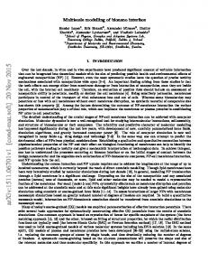
Monte-Carlo simulation of the interface at a macroscale level, with data, associated with interface forces, wear volume and topography evolution for each contact zone, being provided by a microscale model of asperity interaction. The microscale model calculates wear at the asperity level, employing either analytical or numerical models. The data exchange between the macro- and microparts of the model is performed through interpolation on a map at microscale level, computed in advance. This map is based on a standard set of asperity parameters which act as the link between the two models, with the advantage of preserving the full interchangeability between models of the same scale. The simulation can produce two kinds of results, either functions of the friction and wear response of the specific surface at various levels of applied pressure (macrowear mapping), or a set of timeseries of the evolution of tribosystem conditions at a given pressure (macrowear simulation). This model has been used by the authors to predict the results of wear tests of engineering ceramics (14). An adapted multiscale model for a metalforming tribosystem, incorporating full plastic contact and pressure boundary conditions, has also been proposed (15).
INTRODUCTION The science of tribology has as its ultimate goal the accurate prediction of the friction coefficient and wear rate in a tribosystem, based solely on material and surface properties without the need of wear testing (1). This is difficult to achieve, due to the complexity, nonlinearity and cooperative effects of several wear mechanisms, diminishing the effectiveness of the original analytical solutions (2-4); the randomness of morphology and material variables, hindering any deterministic approach; finally, the multiscale nature of wear, being essentially a macroscopic manifestation of cooperative micro- and nanoscale phenomena (5). The generally accepted approach to analytical wear modelling is based on the assumption that wear can be described over the entire interface by a single equation (24), adjusted, in each case, by empirical coefficients (single scale modeling), requiring experimental evidence, see the critical review in Ref. (1). A refinement of this approach is the employment of numerical simulation techniques at the macroscale (component geometry) level, with such a modeling providing increased accuracy in predicting the evolution of wear scars in mechanical components (6). However, it is still confined to the integration of a macroscale wear equation on a space of local values of its variables (usually pressure and sliding velocity) and it does not approach the real scale of the phenomena. On the other hand, most mechanism-based wear models implicitly or explicitly employ some sort of multiscale approach and stochastic representation of the key input variables. Up to date, numerical simulation has seen little application at the microscale (single asperity) level (7–10), due to the problem of randomness and the non-linearity of the associated phenomena. The most elusive aspect is the actual mechanism of wear, i.e. the way a portion of the modelled material is detached and forms wear debris. Also microscale simulations are not parametrised enough to be useful in multiscale modelling.
profile
Materials, work hardening
1. Statistical asperity model
Asperity sample
Computational grid
2. Design Of Experiments
Asperity interaction map
3. Micromodel
Contact sample
A Monte Carlo simulation is a great way to easily perform the integration of stochastic functions in higher dimensional spaces (11). It has been successfully applied in surface mechanics and tribology, where it has been used to integrate analytical models of erosive and abrasive wear (12).
Macrowear mapping: wear coefficient k vs Pressure p
Meshfree methods, such as the Smooth Particle Hydrodynamics (SPH) method, where the flow of nodal masses is not restricted by a mesh, are more suitable than the Finite Element Method in addressing the specific difficulties that arise in a tribosystem. These would be large, non-linear deformations, which cause severe instabilities to mesh-based methods, as well as extensive formation of new surfaces, because of crack propagation, fragmentation and release of wear debris (13).
N times
4. Monte Carlo Simulation
Tribosystem evolution: wear vol. V(t) friction coeff. μ(t) surface statistics work hardening
Figure 1. Model flowchart.
The initial task of the macromodel is to discretise a measured surface profile or roughness parameters into a population of asperities with parametric shape functions. A simple 2D asperity model would describe a profile with 2 parameters, the asperity tip height above the mean profile line z and the asperity radius of curvature R. A further
THE MULTISCALE APPROACH The present work deals with the development of a multiscale model for sliding wear (Figure 1), applying a
2
asperity shape parameter that is of importance is the length of the valley that lies aft of the asperity (xasp). The work hardening of each surface can be represented by the parameter rps (ratio of plastic strain), which is defined as the ratio of the critical depth above which the material has an equivalent plastic strain above a specified value, to the interference δ, assuming that the variation of plastic strain with depth is a monoparametric exponential function. The asperity population thus produced has 4 parameters (h, R, rps, xasp) with distributions that are cross-correlated. Since it isn’t measurable in conjunction with the profile, rps will remain uncorrelated with the other three. To obtain a sample large enough for a Monte Carlo simulation, empirical multivariate distributions of these parameters are calculated from the profile, using continuous kernel estimators and rank correlation. Figure 2. Interaction of BACs during simulation.
The asperity populations involved in friction change with profile separation. When loads increase and separations decrease, the numerous small contact patches merge into fewer larger ones. This effect is known to contact mechanics researchers and corrections to the classical contact mechanics models have been proposed (16, 17). This work takes a more empirical approach. In translating a continuous profile into a sample of asperities, a critical height relative to the profile mean line (zcr) is selected and a circular segment is fitted to all profile segments that protrude above this height. The multivariate distributions are calculated for a wide band of critical levels. In this way, the parametric asperity modelling is able to represent asperities of different scales (sizes) from the same surface, their interaction with the counterface being the criterion by which the relevant scale is selected.
A Monte Carlo simulation is subsequently performed, where the whole sample is in contact in tandem, under the same macroscopic conditions, for N iterations. Each cycle involves one interpolation of the current state of sample geometry parameters into the map, to find the corresponding outputs (wear volumes and contact forces) and the new state for the parameter set. The contact pressure is an external variable imposed by the system macrogeometry; hence it is mapped externally. Pressure has to be calculated iteratively at each cycle, by setting a surface separation d for the two samples, interpolating on the map and then summing the normal force of all resulting interactions. The initial separation d0, used as a first guess to begin the iterations is found by combining the BACs of the two interacting samples at such levels that each bearing area equals the fraction of pressure to material hardness (P/H). All outputs are weighted by the relative sliding distance for each sample asperity; for each cycle an asperity on one side is considered to have sled a distance equal to the sum of asperity and valley lengths (c+xasp) of the asperity it interacts with.
When two parametric asperity populations interact, their interactions form a population of their own. An interaction between two asperities would have 3 parameters: interference δ and the two radii R1, R2. Two surfaces represented as 4-parametric asperity populations (h, R, rps, xasp) will thus be combined into a 5-parametric population of interactions (δ, R1/δ, R2/δ, rps1, rps2). Valley length (xasp) is used in calculating the simulated sliding distance for each asperity. A Bearing Area Curve (BAC) for the asperity population can be constructed (Figure 2) and compared to the profile’s own BAC (the Abbott curve). The interaction of the BACs and the applied pressure determines the separation of the two profiles.
The process is repeated for each iteration with a random permutation of the asperity sample and in the end all N rates are averaged. Therefore, the calculated wear rate corresponds to an instantaneous wear rate, which can be considered as the running-in wear rate if the profile belongs to a pristine surface or as the steady-state rate, if the profile belongs to a run-in surface. Alternatively, the worn population of each step can be used as input to the next one and a transient analysis can be performed, however, as the profile is not resampled based on the changing asperity population, this can cover only the early stages of runningin. MICROSCALE WEAR MODELS Most modern wear models implicitly or explicitly employ some sort of multiscale approach and stochastic representation of the key input variables. The microscale model can be of any type as long as it conforms to the parameters of the macromodel: (a) analytical, based on slip-line field theory equations. (b) semi-empirical, based on generalising the observed
3
mechanisms with parametric equations. (c) based on numerical simulations. The models discussed below have been adapted into the 5parameter framework of the present modeling for comparison with the numerical models. The analytical and semi-empirical models have been mapped on the 5parametric space (h, R1, R2, rps1, rps2) with a uniform grid (of size 3x21x21x7x7) and the numerical models, being computationally intensive, have been calculated at 80 points following the quasi-random Sobol set (18) and interpolated form mapping with cubic Radial Basis Functions (RBFs) (19).
(a)
Adhesive wear A model for adhesive wear has to facilitate the following calculations: for a given load and asperity distribution, find the number and size of junctions, then calculate the normal and traction force profiles of each junction, correct for the effect of rolling or sliding motion, and finally, find the possible locus of the junction fracture surface. The first two steps of this process have been adequately modelled, with the use of stochastic plastic contact mechanics models. Single asperity interaction is being addressed with established adhesive contact models based on specific surface energies, such as that of Derjaguin-Muller-Toporov (20). The last two steps are complicated enough to resist analytical scrutiny.
(b)
This work is basing the comparisons on adhesive wear to the work of Salib et. al. (21), which employs implicit 3D FEM simulations of sphere-on-flat adhesive contacts as a microscale model. The contacts were subjected to traction and incipient sliding conditions in order to calculate the path of least resistance for the formation of a transfer particle, which they did with a copious and non intuitive process (see Appendix 1). This approach incorporates the effect of sliding to the junction area and force profiles, but does not account for the probability that subnominal adhesion, caused by surface chemistry, may not allow the necessary stresses for subsurface crack growth. Hence the predicted wear coefficients are expected to be much higher than the experimental (22).
(c) Figure 3. Slip line fields for the abrasive wear modes: (a) wedge formation, (b) microcutting and (c) wave formation (24). Three abrasive wear models have been implemented (see Appendix 1): (a) The 2D model by Hockenhull et.al. (24), is based on the slip-line field in a deformable halfspace, caused by the contact of a rigid wedge. It is subdivided into three regimes: microcutting, wedge formation and ratchetting (plastic wave). The slip line field for each has a different shape leading to sharp wear transitions (Figure 3). (b) The 3D model by Xie & Williams, (25) is based on an experimental mapping of single asperity wear behaviour. Spherical rigid asperities are interacting with a deformable halfspace by microcutting, ratchetting or ploughing. (c) A simple asperity truncation model, wherein all volume interfering with the cutting asperity is removed and no volume is deformed and displaced.
Abrasive wear The abrasive wear mechanisms are simpler than the adhesive ones because surface chemistry has a lesser role under gross sliding and because the pressure profiles on asperity junctions are easier to calculate. Wear at the asperity level can be calculated using the slip line field theory, adapted to the abrasive conditions by Challen & Oxley (23). What complicates modelling is that wear may not ensue in a single contact event, as it is observed with the microcutting and wedge formation submechanisms, but may come after several contact cycles (each one of them under different conditions) as is the case with ratchetting. Further complications rise from the fact that asperity shape derived properties, like angle of attack are important and also the third dimension (width) is difficult to disregard, because of ploughing.
Microscale simulation The SPH-based numerical model features the same geometry for both the abrasive and the adhesive case. It is 2D plane-strain in order to keep the mapping parameters at a minimum and to reduce the computational cost; however, 3D models can be employed too, if deemed necessary. The SPH elements are deployed in a uniform grid, slightly deformed to assume the asperity shape (Figure 4a). After the contact of the two modeled asperities, the SPH nodes are plastically deformed, with ploughing, microcutting, tensile cracks and debris separation being in the range of the observed results (Figure 4b). For the purposes of
4
automatic post-processing of the model, the wear volume is calculated from a histogram of the node velocities after contact. Details about the micromodel, along with an application in the sliding wear of ceramic materials can be found in (26).
RESULTS Mapping Visualising multidimensional spaces is not easy, however 3-dimensional sections of the mapping for the wear volume of the softer asperities are presented in Figure 5 for adhesion and Figure 6 for abrasion.
(a)
R2/δ
R1/δ (a)
(b) Figure 4. (a) The setup of one SPH simulation: constrained nodes, interference (δ) and sliding diastance (s) are indicated; (b) Classification of SPH nodes into worn/unworn/transferred material. Wear debris formation is observed (abrasive conditions). Different SPH element parts treat each other’s particles in contact as part of their own material, so if there is no third body, e.g. a fluid or solid lubricant, having a small shear flow stress, then the contact is fully adhesive. For abrasive wear, where one part’s hardness is considerably higher than the other’s, the counterface nodes are constrained from deforming and interact with the deformable nodes, with the appropriate corrections in the interaction forces, to prevent adhesion and impose a predefined coefficient of interfacial friction f (defined as the ratio of junction strength to the shear strength of the abraded material: f=τ/k). For both the numerical and the analytical micromodels for the abrasive case, a value of f=0.2 is used, see also Ref. (24).
R1/δ
R2/δ (b)
Figure 5. Adhesive wear volume log(V1) (m3/m) vs log(R1/δ), log(R2/δ) and rps1: (a) 2D numerical (SPH) , (b) 3D semi-empirical.
5
R1/δ
R1/δ
R2/δ (a)
R1/δ
R2/δ (b)
R1/δ
R2/δ (c)
R2/δ (d)
Figure 6. Abrasive wear volume log(V1) (m3/m) vs log(R1/δ), log(R2/δ) and rps1: (a) 2D numerical (SPH), (b) 3D truncation, (c) 2D slip-line, (d) 3D semi-empirical.
The wear coefficients predicted by the numerical simulation (Figure 5a) are considerably higher than those of the analytical adhesive wear model (Figure 5b). In abrasive wear, the results are all of a comparable scale. The slip-line model offers the weakest solution, as it only calculates for a small area of the map (Figure 6c). The 3D models (Figure 6 b,d) show a reverse trend in respect to R1 and R2, which is an artifact of the single asperity wear volume being dependent on asperity width.
Comparison to the results from analytical models Using the same material, AISI-1015 mild steel with hardness H=1285MPa, and the same asperity sample (Ra = 0.4 μm) in all cases, a series of simulations has been performed, at 20 different load points (7 ~ 300 MPa), in order to compare the numerical models with the analytical models examined above. In the abrasive runs, the counterface has the material properties of WC-6%Co (26). The work hardening factor is considered to be normally distributed for both sides: rps=5±1.5. All simulations involve 5000 asperities for 100 cycles. The comparison is based on surface.
6
Wri , the average running-in wear rate on a fresh
(a) Figure 8. Clearance d vs Pressure P.
(b) Figure 7. (a) Dimensionless wear coefficient K vs Pressure P (the 2D slip-line case is too low and is omitted), (b) Variation of K, normalised by the average, Kavg, for the analytical models Figure 7 demonstrates on a logarithmic scale the difference in the dimensionless wear coefficient K for the various models used, as well as its pressure dependence. Figure 8 maps the clearance of the two rough surfaces (the distance between their mean profile lines) as a function of pressure. The numerical microscale models lead the interface to equilibrium at a higher clearance than the analytical models. Figure 9 demonstrates the variation of the friction coefficient with pressure, relative to the average calculated for each model. Table 1 compares results from simulations at a reference pressure of 20MPa, based on maps created by the 5-parameter numerical microscale model and by the analytical microscale models. The average coefficient of friction (μavg) and the average number of contacts are also reported. The average total sliding distance for N=100 cycles is S=20.5mm in all cases and the nominal surface area for 5000 asperities is A=1.02·106 mm2.
Figure 9. Variation of friction coefficient μ vs Pressure P, normalised by the average for each model, μavg. Table 2 summarizes the average dimensionless Archard’s wear coefficient K calculated by each model for 13 load points in the range 7~80MPa. For larger loads, the critical level from which the profile is sampled is lower and the sample asperities are larger, hence the area of the simulated surface is larger.
7
Adhesive 2D SPH
Model Wavg (mm3/m)
Abrasive 2D SPH
Abrasive 2D Slipline
Abrasive 3D Truncation
Abrasive 3D Semi-empirical
2.76E+05
4.15E+01
5.94E-03
3.22E-15
2.28E+03
4.35E+05
0.004
0.43
0.003
-
0.194
0.164
171
172
171
5000
3013
5000
5.23E-03
1.06E+01
7.53E-10
2.02E-22
1.43E-04
2.73E-02
μavg # contacts K
Adhesive 3D Semi-empirical
Table 1. Macroscale simulation for P=20MPa, comparing analytical and numerical microscale models.
Abrasive microscale model
K
Experimental (Ref.24)
7.00E-03
Semi-empirical (3D)
5.03E-02
Slip-line (2D)
2.43E-22
Truncation (3D)
1.70E-04
Abrasive SPH (2D)
2.31E-08
Adhesive microscale model
K
Experimental (Ref.17)
1.50E-02
Semi-empirical (3D)
7.64E+00
Adhesive SPH (2D)
5.81E-03
It is to be noted that, the friction coefficient is independent of pressure in all models, except for the 3D adhesive semiempirical one (Figure 9). Although smoother surfaces have larger contact areas and therefore larger friction in adhesion, it may be considered that the numerical models are predicting an unnaturally low friction coefficient, which is attributed to the shortcomings of the SPH method when the asperities modeled are too smooth (high R1/δ, R2/δ) and is manifest through the Monte Carlo simulation due to the low roughness of the surfaces. The simulation based on the 2D slip line field model map calculates extremely low wear rates, since almost all asperity interactions during the simulations correspond to areas of the map which the model does not cover, since the mapping of this model in the space (f, θ) (23), has undefined areas and also for most interactions of the simulation contact falls in the model’s elastic region. In the adhesive case, the SPH results are closer to the experimental (from (21), mild steel on mild steel) and the analytical model overestimates as expected. The abrasive SPH model grossly underestimates the wear rate and this can be once more attributed to the difficulties the micromodel has with very smooth asperities.
Table 2. Comparison of average wear coefficients for P=7~80MPa.
DISCUSSION The results of the numerical microscale models are more irregular than those of the analytical ones, however they present smoother transitions (Figures 5, 6). The use of an equivalent radius renders the analytical maps symmetric in respect to R1 and R2, however the numerical maps demonstrate the existence of a great dependence on the ratio of the two radii. The wear volume generally increases with the sharpness of the worn asperity; however the sharpness of the wearing asperity (R2/δ) has a reverse effect in adhesion. The worn asperity’s work hardening (rps1) is not taken into account by the truncation model at all and in the other cases it only has a significant effect at low values, when the highly strained area is comparable in thickness to δ. The general trend observed from the simulations (Figure 7) is that in abrasion K increases with P throughout the entire range that can be encountered in engineering surfaces. Mapping at higher pressures (at the upper range of Figures 7-9) indicates that this continues until a significant amount of the surface is work-hardened and the maximum number of asperities gets in contact. This corresponds to the transition described by the formula of the plasticity index in analytical modeling. In adhesive wear, there is a smaller reverse relationship, see Figure 7b, where the trends in normalized K for analytical abrasive and adhesive models are compared. These effects require further investigation, since they may be artifacts of the way the parametric asperity representation, using circular asperities, represents the BAC of the profile.
The wear simulations performed in this work have only comparative purposes, as all the models included are short of predicting the wear rate with the required accuracy. Note, however, that several effects, i.e. thermal, chemical, hydrodynamic lubrication, as well as third bodies, are not taken into account; these require additional equations and more empirical coefficients for their inclusion in analytical modelling. Note, also, that the numerical microscale modelling, is affected by the shortcomings of the 2D representation, whilst, on the other hand, the analytical models can not provide a detailed representation of the worn volume and the topography evolution. Furthermore, macroscale simulation may be sensitive to microscale mapping of the normal load, since it directly affects the surface separation and the number of contacts. Subsequently, future investigations in numerical modelling, for integrating all these effects at the asperity level and providing parametric asperity level wear maps, are needed. One of the advantages that this multiscale model demonstrates is great flexibility in modeling transient effects, at the asperities interface level thanks to the numerical simulation, as well as at the profiles interface level, with the Monte Carlo simulation’s ability to integrate over complex wear transitions. The stochastic approach
8
also provides a framework in which it may be possible to quantify and manage the relative errors that each aspect of the model introduces to the calculation, however this aspect requires further study. Most importantly, the parametric mapping and stochastic simulation approach provides the ability to easily and intuitively increase model complexity and detail, an issue that has always been central to wear modeling.
(8)
(9)
(10)
CONCLUSIONS In this work, a multiscale approach has been employed to model the sliding wear of steel. This model encompasses a combination of novel techniques: A statistical description of surface roughness, based on a multilevel sampling of the profile by empirical multivariate distributions. A Monte Carlo simulation, to integrate the results of the asperity model into their macroscopic counterparts, in a 5-dimensional space. A numerical microscale model of single-asperity interaction, involving friction, wear and plastic deformation with the use of the meshfree Smooth Particle Hydrodynamics method.
(11) (12)
(13)
(14)
This model allowed the comparison of existing analytical microscale models for adhesive and abrasive wear with the numerical microscale simulations. The key findings were: 3-dimensional models are not easily comparable with 2-dimensional ones. The numerical maps demonstrate a dependence of the wear volume on the ratio of the radii of curvature of the two interfacing asperities, an effect discounted by the analytical models. The dimensionless wear coefficient appears to change with pressure, so wear is not linear as supposed by Archard’s law. The wear mechanism is affecting this relationship. The reasons behind this observation require further investigations.
(15)
(16)
(17)
(18)
(19)
REFERENCES (1) Ludema KC. (1996) “Mechanism-based modeling of friction and wear,” Wear, 200, pp.1–7. (2) Archard JF. (1953) Contact and Rubbing of Flat Surfaces. Journal of Applied Physics, 24(8), 981– 988. (3) Archard JF, Hirst W. (1956) The Wear of Metals under Unlubricated Conditions. Proceedings of the Royal Society of London. Series A. Mathematical and Physical Sciences, 236(1206), 397 –410. (4) Rabinowicz E. (1995) Friction and Wear of Materials. Wiley. (5) Cantizano A, Carnicero A, Zavarise G. (2002) “Numerical simulation of wear-mechanism maps,” Computational Materials Science, 25, pp.54–60. (6) Põdra P, Andersson S. (1999) “Simulating sliding wear with finite element method,” Tribology International, 32, pp.71–81. (7) Tworzydlo WW, Cecot W, Oden JT, Yew CH. (1998) “Computational micro- and macroscopic
(20)
(21)
(22)
(23)
(24)
9
models of contact and friction: formulation, approach and applications,” Wear, 220, pp.113– 140. Popov VL, Psakhie SG. (2007) “Numerical simulation methods in Tribology,” Tribology International, 40, pp.916–923. Kermouche G, Rech J, Hamdi H, Bergheau JM. (2010) “On the residual stress field induced by a scratching round abrasive grain,” Wear, 269, pp.86–92. Ko P, Iyer S, Vaughan H, Gadala M. (2001) “Finite element modelling of crack growth and wear particle formation in sliding contact,” Wear, 251, pp.1265–1278. Rubinstein RY, Kroese DP. (2008) “Simulation and the Monte Carlo method.” Wiley-Interscience. Fang L, Xing J, Liu W, Xue Q, Wu G, Zhang X. (2001) “Computer simulation of two-body abrasion processes,” Wear, 251, pp.1356–1360. Belytschko T, Krongauz Y, Organ D, Fleming M, Krysl P. (1996) “Meshless methods: An overview and recent developments,” Computer Methods in Applied Mechanics and Engineering, 139, pp.3– 47. Mamalis AG, Vortselas AK. (2012) Wear of ceramic interfaces: Multiscale statistical simulation. Wear, 294–295, 402–408. Mamalis AG, Vortselas AK, Manolakos DE. (2008) “Multiscale modelling of wear by combined use of numerical and statistical methods.” In Proc. 9th ICTP, Gyeongyu, Korea, pp.223-228. Ciavarella M. (2008) “Inclusion of “interaction” in the Greenwood and Williamson contact theory,” Wear, 265, pp.729–734. Ciulli E, Ferreira L, Pugliese G, Tavares S. (2008) “Rough contacts between actual engineering surfaces:: Part I. Simple models for roughness description,” Wear, 264, pp.1105–1115. Bratley P, Fox BL. (1988) “Algorithm 659: Implementing Sobol’s quasirandom sequence generator,” ACM Trans. Math. Softw., 14, pp.88– 100. Baxter BJ. (1992) “The interpolation theory of radial basis functions,” Doctoral Thesis. Trinity College, Cambridge University. Derjaguin B., Muller V., Toporov Y. (1975) “Effect of contact deformations on the adhesion of particles,” Journal of Colloid and Interface Science, 53, pp.314–326. Salib J, Kligerman Y, Etsion I. (2008) “A Model for Potential Adhesive Wear Particle at Sliding Inception of a Spherical Contact,” Tribology Letters, 30, pp.225–233. Brizmer V, Kligerman Y, Etsion I. (2006) “The effect of contact conditions and material properties on the elasticity terminus of a spherical contact,” International journal of solids and structures, 43, pp.5736–5749. Challen JM, Oxley PLB. (1979) “An explanation of the different regimes of friction and wear using asperity deformation models,” Wear, 53, pp.229– 243. Hockenhull BS, Kopalinsky EM, Oxley PLB.
(1992) “Mechanical wear models for metallic surfaces in sliding contact,” Journal of Physics D: Applied Physics, 25, pp.A266–A272. (25) Xie Y, Williams JA. (1996) “The prediction of friction and wear when a soft surface slides against a harder rough surface,” Wear, 196, pp.21–34. (26) Mamalis AG, Vortselas AK. (2012) “Single
asperity wear modeling of ceramic surfaces using the Smooth Particle Hydrodynamics method,” Journal of Tribology and Surface Engineering, 2, Issue 3-4, #8. (27) Williams J. (1999) “Wear modelling: analytical, computational and mapping: a continuum mechanics approach,” Wear, 225, pp.1–17.
APPENDIX 1 1. Adhesive wear, 3D semi-empirical model by Salib et. al. (21): The results of the incipient sliding FEM simulations were mapped as exponential functions of a dimensionless normal load parameter (P*) and basic material properties (E/Y0 and v). The dimensionless Archard wear coefficient is:
k
22.8v 9.9 P* 0.055exp 410 673v 19
5
E Y0
Ratchetting: [2]
Wedge formation: Cutting:
Cutting:
2
H 0.003 K b f f 2 l H s
[1]
[5]
0.5
, 45 o
0.5
, 45 o
l 1 / 2 (l 0.2) f 2 l 1 / 2 0.2 (l 0.2) where κ, εf are the shear strength and tensile elongation at break of the abraded material, respectively.
sin 2 12 sin 2
2 3 1 sin 2
tan 3 f l 0.5 f
[6]
3 sin sin xy A cos sin 2 C
K
Ratchetting: K 0.225
H tan 3 K 0.003 b f f 2 l H s
2. Abrasive wear, 2D model by Hockenhull et.al. (24): Based on the angles of the slip-line fields of Fig.3:
K
4. Abrasive wear, 3D truncation model: The entire interfering volume is removed. Wear volume per unit width:
[3]
hH 3 3 K P 1 1 2 4 cot 1
Vw
2 ( R / 3) 2 ( R1 R2 )2 ( R1 R2 )2
[7]
In all models the resulting attack angle θ is connected to the interference δ and the equivalent asperity radius R thus:
[4]
3. Abrasive wear, 3D model by Xie & Williams, (25,27): The effect of wear scars partially overlapping in the third dimension is addressed with a stochastic parameter l for the distance between them, one that is following a uniform distribution. In this model wear regime transitions are mapped as functions of l and the asperity attack angle ψ.
2R R
[8] , where R
R1 R2 R1 R2
Under the assumption of half contact during sliding, the normal load for the plastic asperity contact, used in all models, is:
P R
10
Hs 2
[9]