Multistage Schemes With Multigrid for Euler and Navier ... - CiteSeerX

NASA Technical Paper 3631

Multistage Schemes With Multigrid for Euler and Navier-Stokes Equations Components and Analysis R. C. Swanson Langley Research Center • Hampton, Virginia Eli Turkel Tel-Aviv University • Tel-Aviv, Israel

National Aeronautics and Space Administration Langley Research Center • Hampton, Virginia 23681-2199

August 1997

Available electronically at the following URL address: http://techreports.larc.nasa.gov/ltrs/ltrs.html Printed copies available from the following: NASA Center for AeroSpace Information 800 Elkridge Landing Road Linthicum Heights, MD 21090-2934 (301) 621-0390

National Technical Information Service (NTIS) 5285 Port Royal Road Springfield, VA 22161-2171 (703) 487-4650

Contents 1. Introduction . . . . . . . . . . . . . . . . . . . . . . . . . . . . . . . . . . 1 2. Mathematical Formulation . . . . . . . . . . . . . . . . . . . . . . . . . . . . 3 2.1. Equations . . . . . . . . . . . . . . . . . . . . . . . . . . . . . . . . . 3 2.2. Physical Boundary Conditions . . . . . . . . . . . . . . . . . . . . . . . . 5 3. Spatial Discretization . . . . . . . . . . . . . . . . . . . . . . . . . . . . . . 5 4. Arti cial Dissipation . . . . . . . . . . . . . . . . . . . . . . . . . . . . . 13 4.1. Development of Dissipation Form . . . . . . . . . . . . . . . . . . . . . . 13 4.2. Dissipation Model . . . . . . . . . . . . . . . . . . . . . . . . . . . . . 15 4.3. Boundary Treatment of Dissipative Terms . . . . . . . . . . . . . . . . . . 18 4.3.1. Boundary-point operators . . . . . . . . . . . . . . . . . . . . . . 18 4.3.2. Local mode analysis . . . . . . . . . . . . . . . . . . . . . . . . . 20 4.4. Matrix Analysis

. . . . . . . . . . . . . . . . . . . . . . . . . . . . . 22

4.5. The Upwind Connection . . . . . . . . . . . . . . . . . . . . . . . . . . 24 4.6. Matrix Dissipation Model . . . . . . . . . . . . . . . . . . . . . . . . . 25 5. Discrete Boundary Conditions . . . . . . . . . . . . . . . . . . . . . . . . . 27 6. Basic Time-Stepping Schemes . . . . . . . . . . . . . . . . . . . . . . . . . 31 6.1. Runge-Kutta Schemes . . . . . . . . . . . . . . . . . . . . . . . . . . . 31 6.2. Stability of Runge-Kutta Schemes for Systems . . . . . . . . . . . . . . . . 38 6.3. Time Step Estimate . . . . . . . . . . . . . . . . . . . . . . . . . . . . 44 7. Convergence Acceleration Techniques . . . . . . . . . . . . . . . . . . . . . . 46 7.1. Local Time Stepping

. . . . . . . . . . . . . . . . . . . . . . . . . . . 46

7.2. Residual Smoothing . . . . . . 7.2.1. Constant coecients . . 7.2.2. Variable coecients . . . 7.2.3. Removal of diusion limit

. . . .

. . . .

. . . .

. . . .

. . . .

. . . .

. . . .

. . . .

. . . .

. . . .

. . . .

. . . .

. . . .

. . . .

. . . .

. . . .

. . . .

. . . .

. . . .

. . . .

. . . .

. . . .

46 46 49 53

7.3. Multigrid Method . . . . . . . . . . . . . . . 7.3.1. Basic concepts of multigrid methods . . . 7.3.2. Transfer operators . . . . . . . . . . . 7.3.3. Elements of present method . . . . . . .

. . . .

. . . .

. . . .

. . . .

. . . .

. . . .

. . . .

. . . .

. . . .

. . . .

. . . .

. . . .

. . . .

. . . .

55 56 58 59

8. Turbulence Modeling . . . . . . . . . . . . . . . . . . . . . . . . . . . . . 61 9. Concluding Remarks . . . . . . . . . . . . . . . . . . . . . . . . . . . . . 66 Appendix A|Equations for Boundary Points . . . . . . . . . . . . . . . . . . . . 67 Appendix B|Development of Residual Smoothing Coecients . . . . . . . . . . . . 69 Appendix C|Multigrid Transfer Operators

. . . . . . . . . . . . . . . . . . . . 74

References . . . . . . . . . . . . . . . . . . . . . . . . . . . . . . . . . . . 76

iii

List of Figures Figure 1. Finite-volume discretization . . . . . . . . . . . . . . . . . . . . . . . . 7 Figure 2. Alternative integration path for physical diusive uxes . . . . . . . . . . . 10 Figure 3. One-dimensional discretization for three-point cell-centered scheme

. . . . . 12

Figure 4. Boundary-point dissipation . . . . . . . . . . . . . . . . . . . . . . . 19 Figure 5. Physical domain for airfoil calculations . . . . . . . . . . . . . . . . . . 30 Figure 6. Plots of four-stage R-K scheme; (2) = 0; (4) = 1=32; coecients are 1/4, 1/3, 1/2, and 1 . . . . . . . . . . . . . . . . . . . . . . . . 36 Figure 7. Plots of ve-stage R-K scheme; (2) = 0; (4) = 1=32; coecients are 1/4, 1/6, 3/8, 1/2, and 1 . . . . . . . . . . . . . . . . . . . . . . 37 Figure 8. Implicit residual smoothing coecient for two forms of variable coecients . . 52 Figure 9. Structure of multigrid W-type cycle Figure C1. Cells of two grid levels

. . . . . . . . . . . . . . . . . . . 60

. . . . . . . . . . . . . . . . . . . . . . . . 74

iv

Ab stra ct

A class of explicit multistage time-stepping schemes with centered spatial dierencing and multigrid is considered for the compressible Euler and Navier-Stokes equations. These schemes are the basis for a family of computer programs ( ow codes with multigrid (FLOMG) series) currently used to solve a wide range of uid dynamics problems, including internal and external ows. In this paper, the components of these multistage time-stepping schemes are de ned, discussed, and in many cases analyzed to provide additional insight into their behavior. Special emphasis is given to numerical dissipation, stability of Runge-Kutta schemes, and the convergence-acceleration techniques of multigrid and implicit residual smoothing. Both the Baldwin and Lomax algebraic equilibrium model and the Johnson and King one-half equation nonequilibrium model are used to establish turbulence closure. Implementation of these models is described. 1. Intro d ucti on

Computational uid dynamics (CFD) is a multidisciplinary eld involving uid mechanics, numerical analysis, and computer science. The evolution of CFD over the last three decades has fostered a broad range of methods for computing the aerodynamics of ight vehicles. At cruise

ight conditions, a variety of approximate techniques are applied by the aircraft industry when designing ight vehicles. With inviscid and irrotational ow assumptions, versatile and reliable panel methods and nonlinear potential equation solvers are used for aircraft design. To determine viscous eects, either an integral or nite-dierence approach is employed to solve the boundary-layer equations. When the interaction between the viscous and inviscid ow regions is important, the computational procedures for these regions are coupled in either the direct mode (i.e., surface pressure is speci ed) or the inverse mode (i.e., surface shear stress in the case of a solid wall is speci ed). Although these computational techniques are ecient and usually provide reasonable estimates of viscous eects, they can be dicult to implement for three-dimensional (3-D) ows when strong viscous-inviscid interactions occur (such as aircraft wing and body juncture ow). In the past few years, substantial improvements were made on the mathematical models of aerodynamic prediction techniques used for aircraft design. The Euler equations allow rotational eects (i.e., vortical structures) and nonisentropic shock waves and thus provide a better inviscid model for ows over aerodynamic con gurations. The Navier-Stokes equations model weak and strong interactions between viscous and inviscid ow regions without special consideration. Both the Euler and the time-averaged Navier-Stokes equations are currently being introduced into the aircraft design process. Progress in aircraft design can be attributed to several factors. A primary factor is the considerable improvement in the accuracy and eciency of numerical algorithms used to solve the Euler and Navier-Stokes equations. Another factor is the signi cant advancements in computer memory capacity and processing times. Although new technologies in computers and computer science will continue to help decrease processing times, the need still exists for strong eort to increase the robustness, accuracy, and eciency of the ow solvers to allow their use in analysis of complex uid dynamics phenomena and aircraft design. An extensive range of numerical algorithms was developed during the last decade to solve the Euler and Navier-Stokes equations. These numerical algorithms can be classi ed by the type of time-stepping scheme and the type of spatial-discretization scheme used. Both

explicit and implicit time-stepping schemes have been constructed. Explicit schemes require less computational storage and a lower number of operations for time integration, but have a stricter limit on the allowable time step. If temporal and spatial dierencing are decoupled, both schemes are amenable to a variety of convergence-acceleration techniques for steady-state problems. The explicit multistage Runge-Kutta scheme of Jameson, Schmidt, and Turkel (ref. 1) and the implicit approximate factorization (AF) scheme of Beam and Warming (ref. 2) are two schemes that employ temporal and spatial decoupling. The multistage schemes, in conjunction with local time stepping and other convergence enhancements (ref. 3), and the AF scheme, with local time stepping and diagonalization of the implicit operator (ref. 4), are ecient schemes for the Euler equations. Central and one-sided dierencing have been considered for the spatial derivatives in the ow equations. When selecting one type of dierencing over another, it is important to understand the dominating design criterion for central and upwind schemes. When constructing a central dierence scheme, the principal underlying guideline is to minimize the arithmetic operation count while simultaneously maintaining the highest possible accuracy. The multistage schemes and Lax-Wendro schemes (refs. 5{11) are currently the most widely used explicit algorithms with central spatial dierencing. The AF scheme is the most frequently used implicit scheme with centered dierencing. A primary objective of an upwind scheme is to capture ow discontinuities such as shock waves using the minimum number of mesh cells. To accomplish this, many upwind schemes utilize the signs of the slopes of characteristics to determine the direction of propagation of information, and thus, the type of dierencing for approximating spatial derivatives. Two procedures for constructing upwind schemes for hyperbolic systems of conservation laws are the ux vector splitting scheme of Van Leer (ref. 12) and the ux dierence splitting scheme of Roe (ref. 13). Upwind schemes have become popular because of their shock-capturing capability. Generally, upwind schemes represent shock waves with two interior cells rather than the three or four interior cells usually needed by central dierence schemes. However, upwind schemes can require as much as twice the computational eort. Multistage time-stepping schemes with central dierencing for spatial discretization on both structured and unstructured meshes are now being used to solve the Euler equations for ows over complex con gurations, including airplanes (refs. 14 and 15). Members of this class of algorithm have also been extended to allow the solution of the compressible Navier-Stokes equations in both two and three dimensions (refs. 16 and 17). Including convergence-acceleration methods, such as local time stepping and constant coecient implicit residual smoothing (which extends the explicit time step limit), has made these solvers reasonably eective. Signi cant performance improvements are achieved principally by using the multistage scheme as a driver of a multigrid method. The multigrid method involves a sequence of successively coarser meshes and enhances the convergence rate and the robustness of the single-grid scheme. In reference 18, a threestage Runge-Kutta scheme with multigrid was successfully applied to the two-dimensional (2-D) Navier-Stokes equations. Then, both Swanson and Turkel (ref. 19) and Martinelli and Jameson (ref. 20) demonstrated that the type of convergence behavior described in reference 18 could be substantially improved. The multigrid procedure was used to solve ow over a wing (ref. 21). Signi cant performance improvements detailed in reference 21 were obtained (refs. 22 and 23) by closely following and extending the ideas developed in the 2-D solvers (refs. 19, 20, and 24). This paper describes an ecient and versatile class of central dierence, nite-volume multigrid schemes for the 2-D compressible Euler and Navier-Stokes equations. The elements of these schemes are the basis for a family of computer codes ( ow codes with multigrid (FLOMG) series) developed by the authors that are now being used in both industry and universities. These computer codes have been applied to numerous uid dynamics problems over the last 2

several years, and have been employed as an analysis code in airfoil design procedures (ref. 25). The primary purpose of this paper is to discuss, and in many instances, analyze, the components of the schemes in these codes. Sections 2 and 3 of this report give the ow equations and describe the nite-volume formulation for spatial discretization. Three alternatives for numerical approximation of viscous stress and heat ux terms are discussed, and the in uence of grid stretching on numerical accuracy is determined. Section 4 of this report discusses arti cial dissipation. After outlining the historical development of a form for dissipation, the scalar dissipation model frequently used with the present schemes is given in section 4.2. The selection of boundary-point dierence operators is an important consideration for the dissipation model. Suitable operators are given, and how local mode analysis can often provide an evaluation for a proposed boundary-point dierence operator is shown. Analysis based on considering the dissipative character of the discrete system of equations is also performed. Section 4.5 examines the intimate connection between the formulation of an upwind scheme and a central dierence scheme, and a foundation for a matrix dissipation model is established. Section 4.6 describes the matrix dissipation model used with the present schemes. Section 5 discusses the discrete boundary conditions. Section 6 de nes the class of explicit multistage time-stepping schemes considered and summarizes their properties. Next, the stability of Runge-Kutta schemes for systems of equations is examined. Subsequently, a timestep estimate for pseudotime integration of the ow equations is given. Since the temporal and spatial discretizations are decoupled, these explicit schemes are amenable to convergenceacceleration techniques. Section 7 addresses techniques used in this report, including local time stepping, implicit residual smoothing, and multigrid. The initial part of section 7 indicates how the discrete system of ow equations is preconditioned with local time stepping. Section 7.2 rst discusses constant coecients for implicit residual smoothing, and also presents basic properties of residual smoothing. Next, a form for variable coecients for implicit residual smoothing based on stability analysis of a 2-D linear wave equation is introduced. From this form, two dierent formulas for variable smoothing coecients evolve, and these formulas are compared. These variable smoothing coecients still generally require a time-step estimate that depends on a diusion limit. The last part of section 7.2 shows how to use variable smoothing coecients to construct new coecients that can allow removal of the diusion restriction. Section 7.3 describes the basic elements of multigrid methods and delineates the salient features of the present multigrid algorithm. Section 8 discusses turbulence modeling. Both an algebraic equilibrium model and a halfequation nonequilibrium model are considered. Details for implementation of the turbulence models are given. Section 9 states concluding remarks. 2. Ma th em atical Fo rmula tion

In this section the integral form of the full Navier-Stokes equations is de ned. Boundary conditions for the in nite domain problem are then given to complete the general mathematical formulation. Section 3 discusses the discrete analogue of the full Navier-Stokes equations, section 4 introduces the reduced form of these equations that is frequently solved in aerodynamic applications, and section 5 gives boundary conditions for the truncated ( nite) domain problem. 2.1. Equa tion s

Let  denote the density, u and v represent velocity components in the x and y Cartesian directions, respectively; p is pressure, T is temperature, E is speci c total internal energy, and 3

H is speci c total enthalpy. If body forces and heat sources are neglected, the 2-D, unsteady Navier-Stokes equations can be written in conservative form in a Cartesian coordinate system as Z ZZ @ WdV + F 1 n dS = 0 (2:1:1) @t V S where t is time,

V is the region being considered, 23 66 u 77 W=6 64 v 775

3 2 E q 66 uq + pex +  1 ex 77 7 F = 66 4 vq + pey +  1 e y 75 Hq +  1 q 0 Q

and

q = ue x + vey  = xe xex + xye xey + yx ey ex + y ey e y

 @u

@v x = 0  + @x @y  xy =  yx = 0  y = 0 

 @u

@x

 @u @y

+

Q = k rT = k



@v @y

 @T

+



@x

@u 0 2 @x  @v @x

0 2 @v @y

ex +



@T ey @y

1 E = e + (u2 + v 2) 2 p H=E+  Here, ex and e y are unit vectors of the Cartesian coordinate system (x;y), and n is an outwardpointing unit vector normal to the curve S enclosing the region V . Air is the working uid used in this paper. The air is assumed to be thermally and calorically perfect. The equation of state is p = RT (2:1:2) where R = cp 0 cv , and the speci c heats cp and cv are constant. The quantities  and  are the rst and second coecients of viscosity, respectively, and  is taken to be 0 32  (Stokes hypothesis). Either a simple power law or Sutherland's law can be used to determine the molecular viscosity coecient . The coecient of thermal conductivity k is evaluated using the constant Prandtl number assumption. The eect of turbulence is accounted for by using the eddy-viscosity hypothesis. (See section 8 on turbulence modeling.) 4

2.2. Phys ica l Boun dary Con ditions

In the continuum case, either an external or an internal ow problem de ned for an in nite domain is considered. Thus, appropriate conditions at wall boundaries, which are assumed to be solid, must be de ned. Later, in the discrete case, nite domains are de ned. Suitable in ow and out ow boundary conditions must then be de ned. For inviscid ows, the tangency (or nonpenetration) condition q

1n =0

(2: 2:1)

must be satis ed, where q is the velocity vector and n is the unit vector normal to the surface. Now, consider the vector momentum equation 

Dq Dt

= 0r p

(2: 2:2)

where D q=Dt denotes the substantial derivative of q , and r is the gradient operator. Clearly, the substantial derivative of q 1 n must vanish along the surface boundary. Therefore 



@ @t



+ q 1 r (q 1 n ) = 0

(2: 2:3)

If the inner product of the unit normal and equation (2.2.2) is subtracted from equation (2.2.3), then q 1 (q 1 r) n = n 1 rp (2: 2:4) Now, consider the transformation (x; y) ! (;  ), take  (x; y) = constant to coincide with the surface boundary, and note that the contravariant velocity component V = 0 (y =J 01 ) u + (x =J 01) v (where the subscripts mean dierentiation and J is the transformation Jacobian) is zero because of equation (2.2.1). Then, from equation (2.2.4) 1  20x x + y y 1 p + 0y u 0 x v 10vx 0 uy 13 (2: 2:5) p =           x2 + y2 For viscous ows, the nonpenetration condition (eq. (2.2.1)) and the no-slip condition q

1t= 0

(2: 2:6)

(where t is the unit vector tangent to the surface) must be satis ed. In addition, a boundary condition is required to determine the surface temperature. For this boundary condition either the wall temperature is set to a speci ed value or the adiabatic condition Q

1n=0

(2: 2:7)

is imposed, where Q is the heat ux vector given in equation (2.1.1). 3. Sp atial D iscretizatio n

A nite-volume approach is applied to discretize the equations of motion. The computational domain is divided into quadrilateral cells that are xed in time. For each cell, the governing equations can be nondimensionalized and written in integral form as follows: @ @t

ZZ



W

dx dy +

Z

(F dy 0 G dx) =

@

5

p M Z Re

@

(Fv dy 0 Gv dx)

(3:1)

where is a generic cell (or cell area) with @ the cell boundary. In the scaling factor for the viscous terms on the right side ofequation (3.1), the quantities , M , and Re are the speci c heat ratio, Mach number, and Reynolds number, respectively, with M and Re de ned by nominal conditions. These factors arise because of the choice of nondimensionalization of the equations. The ux vectors are de ned by 2 3 u

66 u2 + p 77 F= 6 6 uv 77 4 5 uH

2 v 3 66 uv 77 G= 6 6 v 2 + p 77 5 4 vH

2 6 Fv = 6 6 4 2 6 6 Gv = 6 4

0

x  xy

ux + v xy

3 7 77 5 @T

0 k @x

0

yx y

uyx + vy 0 k

@T @y

3 77 7 5

The independent variables x, y , and t are nondimensionalized as ~x x= ~ lref ~y y= ~lref ~u t = ~t ref ~lref p

where u~ ref = ~pref=~ref , and the tilde in this section represents a dimensional variable. Examples of a reference length are the chord for an airfoil and the throat height for a nozzle

ow. The thermodynamic variables p, , and T and the transport coecients  and k are nondimensionalized by their corresponding quantity evaluated at some reference condition. The velocity components are scaled by u~ref , and the total quantities E and H are scaled by u~ 2ref . For external ows, the nominal conditions are based on free-stream values, and for internal ows, the nominal conditions are based on stagnation values. Partition the computational region with quadrilaterals and apply equation (3.1) to each quadrilateral. This process is equivalent to performing a mass, momentum, and energy balance on each cell. A system of ordinary dierential equations is obtained by decoupling the temporal 6

and spatial terms. In particular, consider an arbitrary quadrilateral ( g. 1, ), and approximate the line integrals of equation (3.1) with the midpoint rule. Let the indices ( ) identify a cell. Then, by taking W as the cell-averaged solution vector, equation (3.1) can be written in semidiscrete form as ABC D

i; j

i; j

(

d

i ;j

dt

W

i; j

) + LW = 0

(3 2) :

i; j

where is the area of the cell, and L is a spatial discretization operator de ned by referring to convection, diusion, L = L + L + L , with the subscripts , , and i; j

C

D

AD

and arti cial dissipation, respectively. The convective uxes at the cell faces are obtained by an averaging process. The convective ux balance is computed by summing over the cell faces as C

D

AD

L

C

W

i ;j

=

X4 (F ) 1 =1

C

l

(3 3)

S

:

l

l

with the ux tensor associated with convection given by (F ) = F e + G e and for each cell face , the directed length S is expressed as S = (1 ) e 0 (1 ) e (3 4) where the proper signs of (1 ) and (1 ) produce an outward normal to the cell face. The augmented, convective ux tensor is evaluated as (3 5) (F ) = 12 (W 0q0 + W +q +) + C

l

l

l

x

l

y;

l

y

l

x

y

l

C

l

x

x

l

:

y

l

l

l

P

:

l

B' C' B j+1

C A' D' j

A D

j-1

i-1

i

Figure 1. Finite-volume discretization. 7

i+1

where

Pl =

3

2

0 (pavg )l e x (pavg)l ey ((pq)avg)l T (pavg )l = 12 (p0 + p+ )l ((pq )avg )l = 12 (p0q 0 + p+q +)l and the superscripts minus (0) and plus (+) indicate quantities taken from the two cell centers adjacent to the edge l. The symbol q denotes the velocity vector. In this section, the subscript avg always refers to the simple average de ned in equation (3.5) for a given edge l. The contribution of the diusive uxes in equation (3.2) is evaluated as L D Wi;j =

4 X l=1

(FD )l 1 Sl

(3:6)

where Sl is given by equation (3.4), and (FD )l = (Fv )l e x + (Gv )l e y. First-order spatial derivatives are in the ux vectors Fv and Gv . In the present nite-volume method, these derivatives are determined using Green's theorem. For example, consider the cell face BC in gure 1. The contributions ux and uy to the viscous ux across BC are approximated by their mean values as follows: ZZ (ux)i;j +1=2 = (ux)BC = 10 0 ux dx dy

Z 1 = 0 0 u dy (3:7) @

0 1

0 1

uy i;j+1=2 = uy BC =

1 ZZ u dx dy

0 0 y

Z 1 = 0 0 0 u dx @

(3:8)

where 0 is the area of an appropriate auxiliary cell. Three alternatives for computing the diusion-type terms have been considered. The rst two approximations for a diusive ux are obtained with nite-volume methods, and the third approximation is determined with a frequently used method based on a local transformation of coordinates. A comparison is now made between these three choices. For the comparison, consider the molecular transport processes associated with cell face BC for the x-momentum equation only. Let 8BC = [(FD )BC 1 SBC ] 2 = 0x 1y 0 yx 1x1BC . In one nite-volume method the integration path A0B 0C 0 D 0 ( g. 1) used in references 16 and 26 is considered. Applying the midpoint rule for the required line integrals results in 2

3

8BC =  avg0 1ui;j+1 +  2ui;j +  3uB +  4uC 2 3 +  avg0  5vi;j +1 + 6 vi;j + 7 vB + 8 vC 8

(3:9)

where

4 1y 1y 0 0 + 1x 1x 0 0 BC BC 3 BC B C 4 2 = 1yBC 1yD 0 A0 + 1 xBC 1xD0 A 0 3 4 3 = 1yBC 1yA 0 B0 + 1xBC 1 xA 0 B0 3 4 4 = 1yBC 1yC 0 D0 + 1xBC 1xC 0 D 0 3 2 5 = 1yBC 1xB0 C0 0 1xBC 1y B0 C 0 3 2 6 = 1yBC 1xD0 A 0 0 1xBC 1 yD0 A 0 3 2 7 = 1yBC 1xA0 B0 0 1 xBC 1yA 0 B0 3 2 8 = 1yBC 1xC0 D 0 0 1xBC 1yC 0 D 0 3 1 10 uB = ui;j + ui +1;j + ui;j +1 + ui +1;j +1 4 0 1 1 uC = ui;j + ui 01;j + ui;j +1 + ui 01;j +1 4 1 =

with vB and vC de ned similarly, and 1xBC = xC 0 xB 1y BC = yC 0 yB 1 10 avg =  i;j + i;j +1 2 0 1

0 = 12 i;j + i;j +1 Martinelli (ref. 27) introduced a dierent integration path for calculating the viscous terms (delineated as BFC E in g. 2). Integrating around the boundary BF CE with the trapezoidal rule results in     1 4 2 2 8BC = 2 00 3 1y BC + 1xBC (ui;j +1 0 ui;j ) 0 3 1xBC 1yBC (vi;j+1 0 vi;j )    avg 4 + 2 00 3 1yEF 1yBC + 1xEF 1xBC (uB 0 uC )

avg



avg

+ 2 00



2 1x 1y 0 1y 1x  (v 0 v ) BC B C EF 3 EF BC 9

(3:10)

F

B C

E A D

Figure 2. Alternative integration path for physical diusive uxes.

where

1xEF = 1y EF =

xi;j +1 0 xi;j yi;j +1 0 yi;j

and 00 is the area of the region enclosed by BF CE . The area 00 is given by

00 = 12 (1xCB 1y EF 0 1xEF 1yCB ) All other quantities in equation (3.10) are de ned the same as in equation (3.9). The form of 8BC given by equation (3.10) is much more compact, requiring fewer arithmetic operations than the form of 8BC given by equation (3.9). A third approach for computing the diusion-type terms is based on a local transformation from Cartesian coordinates (x; y) to arbitrary curvilinear coordinates (; ). Derivatives with respect to x and y are expanded according to the chain rule for partial dierentiation. The resulting relation for 8BC is as follows: avg

8BC = 0

 4



2

 

3 1y CBy + 1xCB x u + 3 1y CBx 0 1xBC y v BC 2  4    avg + 0 3 1y BCy + 1xBCx u + 3 1yBC x 0 1xBC y v (3:11) BC

where

x y x y

= 1xCB = 1y CB = 1xEF = 1y EF 10

With a uniformly spaced computational domain (1 = 1  = 1), 8BC in equation (3.11) is the same as 8BC in equation (3.10), except for the area factor. For a Cartesianmesh, the expressions for 8BC in equations (3.9), (3.10), and (3.11) are equivalent. If the streamwise-like dierences associated with the viscous ux quantities are neglected, which is the thin-layer Navier-Stokes assumption, only the terms inside the rst set of brackets are retained. Note that with the thin-layer formulation, there are viscous contributions to the uxes at faces BC and DA only. The following vector approximates the integrand of the right side of equation (3.1) at cell faces BC and DA : 3 2 0 1 7 8l = 64 5 2 ~ l uavg 1 + vavg 2 + Q where 0 1  1 = avg 1u 0 2 v

avg 0 1  2 = avg 3v 0 2 u

~=

Q

avg  

 avg 4 T P r avg 0 1 4 y2 + x2

=3   1 2 = x y 3 4 3 = x2 + y2 3 1

4

= x2 + y2

Unless otherwise indicated in the text, the thin-layer form of the equations is solved. Signi cant dierences in the numerical solutions have not been observed when applying the three methods for approximating the diusive terms. Notable dierences in the numerical solutions were not expected when solving the Navier-Stokes (thin-layer or full) equations on suciently smooth meshes (i.e., meshes without kinks or sudden jumps in mesh intervals). In this paper the integration path of Martinelli (ref. 27) is used in the nite-volume method for computing the viscous uxes. With this choice of integration path (ref. 27), the mean values of the viscous stresses for a given cell edge are obtained at the midpoint of the edge, even when there is a kink in the grid. This is not true for the path used in equation (3.9). Also, with the integration path of equation (3.10), there are fewer arithmetic operations required than with the path of equation (3.9). Theoretical estimates of the order of accuracy of the cell-averaged scheme are now introduced based on one-dimensional (1-D) analysisusing Taylor-series expansions. Consider the coordinate grid around the location denoted by the index i ( g. 3). Let  be a test function. The numerical values of the rst and second derivatives of this function are then given by 2 2 (3:12) (x)num = 12 x 1 x+1+x1x0 + 14 xx 1x+10x1 x0 + O (1x2 ) 11

∆x–

∆x+

i–1 ∆x– –

i

i+1

∆x

∆x+ +

Figure 3. One-dimensional discretization for three-point cell-centered scheme.

and 1 x2+ 0 1x20 1 x+1x0 1 1 (xx)num = 2  xx 1x + 6  xxx 1x 3 3 + 241  xxxx 1x+1+x1x0 + O(1x3 )

(3:13)

respectively, where the derivatives in the expansions are evaluated at i. The approximations of equations (3.12) and (3.13) are zeroth-order accurate on arbitrarily stretched meshes. However, assuming a constant stretching factor of the grid (i.e., = 1x++ =1x = constant), the following relations are obtained: 9 > 1x = 1x 1 > 00



> > > > > > > > > =

 1 1 x0 = 2 1x 1+ 1 (3:14) > > > > 1x++ = 1x > > > > > > 1 ; 1 x+ = 2 1x (1 + ) > For viscous ows, grids with constant stretching factor are often used. If these grids are re ned by doubling the number of points, then p 01 f = c < 1 + c 2 where  1 and the subscripts f and c refer to ne and coarse grids, respectively. To estimate the error reduction when re ning the stretched mesh, the approximation

 1+ C 1x

(3:15)

is used. Then, if the quantities in equations (3.14)and (3.15)are substituted into equations (3.12) and (3.13), respectively, the result is 0 1 ( x)num =  x + 14  x C 1x 2 + 12 C xx 1x2 + O (1x2) (3:16) 12

and

0 1 (xx)num = xx + 14 xx C 1x 2 + 13 C xxx 1x2 + 121 xxxx 1x2 + O(1x3 )

(3 :17)

respectively, for 1x > = > > ;

(4: 2:5)

where u and v are Cartesian velocity components, and c is the speed of sound. The coecients and "(4) use the pressure as a sensor for shocks and stagnation points, respectively, and are de ned as 9 (2) (2) max( =  ; i;j ;i +1;j ; i+2;j ) > " > i 0 1 ;j i +1=2;j >

"(2)

i;j

(4) i +1=2;j

"

=

01;j 0 2pi ;j + 01;j + 2pi ;j +

pi p i

h

> > > > =

pi +1;j pi +1;j i

= max 0; ((4) 0 "i(2) ) +1=2;j

> > > > > > > ;

(4: 2:6)

where typical values for the constants (2) and (4) are in the ranges 1=4 to 1=2 and 1=64 to 1=32, respectively. This paper shall refer to equations (4.2.1) and (4.2.6) as the Jameson, Schmidt, Turkel (JST) scheme (or dissipation model), and shall designate  as the JST switch. It should (2) be mentioned that in reference 1, the coecient "i(2) +1=2;j =  max(i;j ;i +1;j ). The switching function  can be interpreted as a limiter, in the sense that it activates the second-dierence contribution at extrema and switches o the fourth-dierence term. Moreover, at shock waves, the dissipation is rst order, and a rst-order upwind scheme is produced for a scalar equation. In smooth regions of the ow eld the dissipation is third order. Thus, two dierent dissipation mechanisms are at work, and the switch determines which one is active in any given region. For smooth ows,  is small, and the dissipation terms consist of a linear fourth dierence that damps the high frequencies the central dierence scheme does not damp. This dissipation is useful mainly for achieving a steady state and is less important for time-dependent problems. In the neighborhood of large gradients in pressure,  becomes large and switches on the second-dierence viscosity while simultaneously reducing the fourthdierence dissipation. This viscosity is needed mainly to introduce an entropy condition so that the correct shock relationships are satis ed and to prevent oscillations near discontinuities. For subsonic steady-state ow, this viscosity can be turned o by choosing (2) = 0. The isotropic scaling factor of equation (4.2.4) is generally satisfactory for inviscid ow problems when typical inviscid ow meshes (i.e., cell aspect ratio O (1)) are used. The isotropic scaling factor can create too much numerical dissipation in cases of meshes with high-aspectratio cells. The adverse eect of high-aspect-ratio cells is an important consideration for high Reynolds number viscous ows, where a mesh providing appropriate spatial resolution can have cell aspect ratios O(103 ). In an eort to improve this cell aspect ratio situation and obtain sharper shock resolution on a given grid, Swanson and Turkel (ref. 19) replaced the isotropic scaling factor of equation (4.2.4) with the anisotropic scaling factor i+1=2;j

A similar scaling is used in the



=

i 1h ( )i ;j + ( )i +1;j 2

(4: 2:7)

direction.

The anisotropic scaling idea was motivated by the scaling of dissipation occurring in dimensionally split, upwind schemes (i.e., the ux vector split scheme (ref. 12) and the approximate Riemann solver (ref. 13)). Anisotropic scaling is often referred to as individual eigenvalue scaling. While the accuracy is improved with equation (4.2.7), particularly with respect to shock resolution, individual eigenvalue scaling in the streamwise ( ) direction can be too severe for a standard multigrid algorithm. Moreover, the eectiveness of the multigrid driving scheme in damping high frequencies in the  direction can be signi cantly diminished, resulting in a much slower convergence rate. 16

An alternative to the individual eigenvalue scaling was proposed by Martinelli (ref. 27), and considered by Swanson and Turkel (ref. 19). This modi ed scaling factor, which is a function of mesh-cell-aspect ratio, is de ned as 1  ) + ( ) ] (4: 2:8) i+1=2;j = [(  i +1;j 2  i ;j where ( )i;j =  i;j (r ) ( )i;j 9 = (4: 2:9)  ;  i;j (r ) = 1 + r i;j Here, r is the ratio  = , and the exponent  is generally taken to be between 1=2 and 2=3. In the normal direction (), ()i ;j = i;j (r 01)()i ;j is de ned. Thus, the scaling factor of equation (4.2.8) is bounded from below by equation (4.2.7), and bounded from above by equation (4.2.4). As demonstrated in references 19 and 20, the scaling factor of equation (4.2.8) produces a signi cant improvement in accuracy for high-aspect-ratio meshes, and permits good convergence rates with a multigrid method. The scheme in this paper uses this modi ed scaling factor. The impact of the dissipation form on the energy of a system of ow equations is now examined. For simplicity, consider the 1-D, time-dependent Euler equations, with numerical dissipation terms given by J

where

01 @ W + @ F = D2 W 0 D 4W @t



@



(4: 2:10)

 @W  " (2) @   @  @3 W  @ 4 D W = " (4) @  3 @ 2 D W =

@

and "(2) = "(2), "(4) = "(4) , and J 01 is the inverse transformation Jacobian. Form the inner products of W T , with T denoting transpose, and both sides of equation (4.2.10), and then integrate over a domain . After integration by parts and neglecting boundary terms, the equation 1 @ k Wk2 = ux term + J hI (2) 0 I (4)i (4: 2:11) 2 @t is obtained, where Z kWk2 = W2 d

 2 Z (2) = 0 "(2) @ W d I @

 @ 2 W 2 Z Z @ "(4) @ WT !  @ 2W  (4) = 0 "(4) 1 @2 d I d + @2 @ @



The second-dierence dissipation term I (2) only decreases the L 2 norm of the solution vector (i.e., it decreases the energy of the system), and thus, is strictly dissipative. The fourth-dierence dissipation term I (4) contains a dispersive part and a dissipative contribution. 17

An alternative form for the third-order dissipation term (the last term in eq. (4.2.10)) is  @2W  @2 4 "(4) @ 2 D W = @ 2

which can be written in the discrete case as h (4) i 4 D Wi = r 1 (i "i )r 1 Wi

(4: 2:12)

This modi ed form produces only dissipative contributions. If Qi = i "i(4)r 1  Wi , then r 1  Qi = Q i+1=2 0  Qi 01=2 , where  is the standard, centered-dierence operator. Therefore, the form of equation (4.2.12) is conservative, provided  and "(4) are evaluated at the cell centers rather than at the cell faces. In reference 19, numerical tests were performed with the dissipation terms of equations (4.2.3) and (4.2.12). For steady state, there seems to be no consistent bene t for either convergence or accuracy when using the form of equation (4.2.12). Based on these results, the form of equation (4.2.3) is still used. However, for unsteady ows, equation (4.2.12) may oer an advantage because of the absence of dispersive eects that can cause phase errors. Until now, a scalar viscosity in which the viscosity is based on dierences of the same quantity advanced in time has been considered. (See eq. (4.2.10).) The disadvantage is that the total enthalpy is no longer constant in the steady state, even when total enthalpy should be identically constant for the inviscid equations. The total enthalpy is constant for the steady-state Euler equations because the energy equation is a constant multiple of the continuity equation when H is constant. Hence, reference 1 suggests that the dissipation for the energy equation be based on dierences of the total enthalpy rather than the total energy. Thus, a typical situation in one dimension is to replace equation (4.2.10) for the energy equation by 01 @E + @ ( Hu) = D2 (H ) 0 D 4(H ) (4: 2:13) J @t



@



where  H =  E + p. Reference 33 shows that equation (4.2.13) indeed yields a constant total enthalpy, but thatthe entropy tends to be less accurate than if the dissipation term forthe energy equation is based on dierences of  E rather than H . Thus, both choices have advantages and disadvantages. The total enthalpy formulation is used in this paper. 4.3. Bou nd ary Trea tment of Dis sipa tive Terms

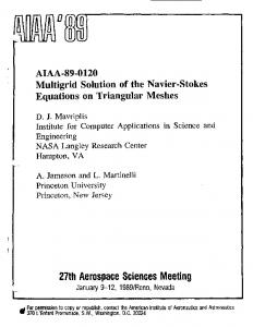
In acell-centered, nite-volume method, the rst andlast cells in each coordinate direction are auxiliary cells where the ow equations are usually not solved. The solution in these cells is found by a combination of the given physical boundary conditions and numerical boundary conditions. Thus, there is no diculty evaluating the second-dierence dissipation term at the rst or last interior cell in a given coordinate direction. In the case of the fourth-dierence dissipation term, the treatment must be modi ed at the boundaries of the physical domain because only one layer of auxiliary cells is considered. Moreover, the standard ve-point dierence stencil must be replaced at the rst two interior mesh cells relative to a wall boundary; thus, one-sided or one-sided biased stencils are used at these cells. The dissipative character of these stencils is important because it in uences both stability and accuracy. For example, if the dissipation is too large at a solid boundary, an arti cial boundary layer is created in an inviscid ow, and the eective Reynolds number for a viscous ow is altered. 4. 3. 1. B oundary-point operators. Inthis section, the two types ofdiscrete boundary-point operators (dierence stencils) used with the present scheme for solid surfaces are de ned. 18

j = 7/2 j=3 j = 5/2 j=2 j = 3/2

j = 1/2

Figure 4. Boundary-point dissipation.

Next, these operators are evaluated by applying a local mode analysis. In addition, this section shows how this local mode analysis can provide an evaluation of candidate boundarypoint operators once a basis for comparison is established. A more complete analysis for the boundary-point operators is based on the dissipation matrix for the system of dierence equations approximating the governing ow equations. Sometimes the dissipation matrix can be characterized analytically. In general, the eigenvalues of the dissipation matrix must be determined. The approach for analyzing the dissipation stencils is discussed. Consider the total dissipation resulting from a numerical ux balance for a mesh cell in a particular coordinate direction. Let wj and d j denote a component of the solution vector W and the corresponding total dissipation, respectively. The index j indicates the mesh cell being considered. Let d j+1=2 and d j01=2 represent the dissipative uxes at the cell interfaces j + 1=2 and j 0 1=2, respectively ( g. 4). At a cell interface (for example, j +1=2), let (1w)j +1=2 denote the dierence between the solution for the adjacent cells (wj+1 0 wj ). For simplicity, assume "(4) = 1. Then, for any cell j (4: 3:1) dj = dj +1=2 0 dj 01=2 where the dissipative uxes are dj +1=2 = (1w)j+3=2 0 2(1w)j +1=2 + (1w)j 01=2 dj 01=2 = (1w)j+1=2 0 2(1w)j 01=2 + (1w)j 03=2 Thus or

d j = (1w)j+3=2 0 3(1w)j +1=2 dj = wj +2

+ 3(1 w)j 01=2 0 (1w)j03=2

(4: 3:2)

0 4wj +1 + 6wj 0 4wj01 + wj 02 Consider the rst two interior cells adjacent to a solidboundary ( g. 4). The total dissipation for these cells is denoted by d 2 and d3 . At j = 2, a value for (1w)1=2 must be determined because 19

(1w)1=2 is unde ned. Also, in this formulation of the boundary-point dissipation stencil, no functional dependence on w1 is desired because w1 is outside the domain. Hence, a value for (1w)3=2 must also be provided. If ) (1w)1=2 = (1w)5=2 (4: 3:3) (1w) = (1w) 3=2

then equation (4.3.2) gives

5=2

d 2 = w4 0 2w3 + w2

(4: 3:4) d3 = w5 0 4w4 + 5w3 0 2w2 (4: 3:5) These boundary stencils are fairly standard and are used for inviscid ow calculations. An alternative form, which reduces the sensitivity to solid-surface, normal mesh spacing for viscous

ow calculations without compromising stability or convergence, is obtained by replacing (1w)1=2 with (1w)1=2 = 2(1w)3=2 0 (1w)5=2 and leaving (1w)3=2 unchanged. This form is given by (4: 3:6) d2 = w4 0 3w3 + 3w2 0 w1 d3 = w5 0 4w4 + 6w3 0 4w2 + w1 (4: 3:7) For turbulent ows, this boundary dissipation formulation (eq. (4.3.7)) is advantageous when the mesh is ne enough to adequately represent the laminar sublayer region of the boundary layer (i.e., at least two points are inside the sublayer). For coarse meshes, this treatment of the dissipation can be less accurate than the zeroth-order extrapolation of equations (4.3.3).

. A local mode analysis is now considered to evaluate the relative damping behavior of boundary-cell dierence operators. For comparison purposes, the interior fourth dierence is rst characterized. Taking a Fourier transform of equation (4.3.2) yields zj () = 4(cos  0 1)2, where zj () is the Fourier symbol of the transformed dj , and  is the product of the wave number and the mesh spacing. Then, zj ()  4 for small , and zj () = 16. The dissipation of long wavelengths is dictated by the behavior of zj () at small , and the dissipation of short wavelengths is governed by zj (). As mentioned initially in this section, this simple analysis assumes that "(4) = 1. In practice, the coecient (4) used in the evaluation of "(4) for the fourth-dierence dissipation aects the behavior of the boundary dissipation stencil. The coecient (4) is chosen such that the highest frequency is highly damped according to a stability analysis using the interior-point stencil. This is important for a multigrid method and will be discussed in section 7.3. Near a boundary, the dissipation should behave in a similar manner. In this dissipation model, the same value of (4) used for interior points of the domain is also used near a boundary. A general form of the dierence stencils at j = 2; 3 can be written as dj = wj+2 0 wj+1 + ( + 0 )wj 0 wj 0 1 4. 3. 2. Local

mode analysis

The associated Fourier symbol is given by zj () = [ + 0 2(1+ cos )] (1 0 cos ) + i ( 0 + 2  cos )sin  20

For small  this Fourier symbol is replaced by

and at  =  reduces to In the case of equation (4.3.4)

2

4

 +  2 2 + i(2 0 + ) 0 i3

(4: 3:8)

zj () = 2( + )

(4: 3:9)

zj () = ( + 0 4)

z2 ( ) 

4

3

2 0 i for small , with z2( ) = 4, and for equation (4.3.5)

(4: 3:10)

2

3 (4: 3:11) 2 0 i for small , with z3( ) = 12. Note that z2 () and z3() are not real. Thus, there are both dissipation and dispersion near the boundary. For the stencil of equation (4.3.6) z3 ( ) 

4

3 (4: 3:12) 2 0 i for small , with z2( ) = 8, and for the stencil of equation (4.3.7) z3()  4 (4: 3:13) for small , with z3() = 16. Comparing equations (4.3.10) and (4.3.12), which correspond to the stencils of equations (4.3.4) and (4.3.6), respectively, shows that both stencils behave the same for the long wavelengths, while equation (4.3.12) is twice as dissipative for the short wavelengths. At j = 3, the stencil corresponding to equation (4.3.13) is fourth order on the long wavelengths, whereas the stencil associated with equation (4.3.11) is only second order. In addition, the symbol of equation (4.3.13) is more dissipative on the short wavelengths. Thus, the improved accuracy and high-frequency damping observed for the stencils of equations (4.3.6) and (4.3.7) in practice is substantiated with this simple analysis. The method of combining the simple local mode analysis with the evaluations just considered to quickly evaluate candidate dissipation stencils can now be shown. Consider a dierent set of boundary-point stencils. If 1w is taken to represent either the component u or v of the solution vector W, and the antisymmetry constraint (1w)1=2 = (1 w)5=2 is imposed for viscous

ows, then equation (4.3.2) gives d2 = w4 0 5w3 + 7w2 0 3w1 (4: 3:14) d3 = w5 0 4w4 + 6w3 0 4w2 + w1 (4: 3:15) The Fourier symbols of equation (4.3.14), using equations (4.3.8) and (4.3.9), are z2()  22 (4: 3:16) for small , with z2( ) = 16, and the symbols for equation (4.3.15) are the same as given in equation (4.3.13). Comparing equation (4.3.16) with equation (4.3.12) shows that the highest frequency is damped better with the proposed stencil, but that the proposed stencil is only second z2 ( ) 

21

order on the long wavelengths, while the stencil of equation (4.3.6) is fourth order, indicating that better accuracy is obtained with equations (4.3.6) and (4.3.7). The improved accuracy has been veri ed with numerical experiments (i.e., skin-friction solutions for turbulent airfoil ows have been computed on 160 by 32 meshes and compared with high-density-mesh results). 4.4. Matrix Ana lysis

The associated dissipation matrix is examined to determine the numerical dissipativity of a discrete system of equations, such as equation (3.2). For simplicity, consider the 1-D system = D(4) w

dw dt

(4: 4:1)

where w is a discrete solution vector, and D(4) is a dissipation matrix corresponding to fourth-dierence terms. Taking the inner product w (the transpose of w ) with each side of equation (4.4.1), obtain 1=2 dw2 =dt = w D(4)w . If the quadratic form w D(4)w is nonpositive de nite, then the matrix D(4) is strictly dissipative. Moreover, the energy of the system is nonincreasing. Assume there are boundaries at j = 3=2 and j = jl + 1=2, and assume j = 2 and j = j l are the indices for the rst and last interior points, respectively. Apply the boundary point stencils of equations (4.3.4) and (4.3.5) at the rst two interior cell centers at both boundaries, and the standard stencil everywhere else. The resulting dissipation matrix is given by T

T

2

01

6 6 2 6 6 01 6 6 6 0 6 6 (4) =6 D 6 6 6 6 6 6 6 6 6 4

2

05 4

01

T

3

01

7 7 7 7 01 7 7 7 4 01 7 7 7 . .. .. . . . . 7 7 7 4 06 4 01 0 7 7 01 4 06 4 01 777 0 1 4 0 5 2 75

01

4

06

4

06

4

.. .

...

01

01

(4: 4:2)

01

2

and the corresponding solution vector is given by w

=[

2

w

3

w

Then w

T

(4)w D

4

5

w

=0

w

01 0 X

jl

:: :

+1 0

wj

=3

wjl

02

wjl

01

wjl

1 2w + w 01 2  0 j

j

]

T

(4: 4:3)

j

Thus, D (4) is strictly dissipative. This same result is obtained by Eriksson and Rizzi (ref. 34). For a 10 by 10 matrix with the form of equation (4.4.2), Pulliam (ref. 35) obtains two zero eigenvalues. Ideally, D (4) should have no zero eigenvalues, since zero eigenvalues can possibly produce undamped modes that cause instabilities (ref. 35). Pulliam (ref. 35) recommends applying a stencil with the weights of equation (4.3.5) at the rst interior cell, and a standard stencil with the weights of equation (4.3.7) at the second interior cell. Then 22

2

05

6 6 4 6 6 01 6 6 6 0 6 6 (4) = 6 D 6 6 6 6 6 6 6 6 6 4

3

01

4

06

06

4

01

7 7 7 7 01 7 7 7 4 01 7 7 7 . .. .. . . . . 7 7 7 4 06 4 01 0 7 7 01 4 06 4 01 777 0 1 4 0 6 4 75

01

4

4

06

4

.. .

...

01

01

4

(4: 4:4)

05

and w

T

(4) w = D

0

01 0 X

jl

wj j

=3

+1 0 2wj

0( 30 2 w

+ w 01

12

j

2 2 2 ) 0 (wj l0 1 0 2wj l)

w

0

(4: 4:5)

Again, the dissipation matrix is strictly dissipative. Moreover, a 10 by 10 matrix with the structure of equation (4.4.4) has zero eigenvalues (ref. 35). However, indications are that for a cell-centered, nite-volume formulation, this boundary-point treatment of the dissipation with the weights of equations (4.3.5) and (4.3.7), although appropriate at in ow and out ow boundaries, is generally too dissipative at solid boundaries. Thus the stencils of equations (4.3.4) and (4.3.5) are preferred at a wall boundary. Now consider the stencils with the weights of equations (4.3.6) and (4.3.7). The dissipation matrix is given by 2

03

01

3

6 6 4 6 6 01 6 6 6 0 6 6 (4) = 6 D 6 6 6 6 6 6 6 6 6 4

06

4

06

4

01

3

4

4

06

.

.

..

7 7 7 7 01 7 7 7 4 01 7 7 7 . . .. . . 7 . . . 7 7 4 06 4 01 0 7 7 01 4 06 4 01 777 0 1 4 0 6 4 75

01 ..

01

01

3

(4: 4:6)

03

and w

T

D

(4) w

=0

01 0 X

jl

wj j

=3

+1 0 2wj

0 ( 01 0 w

jl

w

1 + w 0 1 2 + w2 (w3 0 w2 ) 0 (w3 0 w2)2 j

)2 + w (w

jl

jl

23

jl

0

w

01 )  0

jl

(4: 4:7)

From the quadratic form of equation (4.4.7), it does not directly follow that D(4) is nonpositive de nite, which is generally the case with the quadratic form. If the eigenvalues of a 10 by 10 matrix with the structure of equation (4.4.6) are determined, one is zero and the others are negative. Therefore, the matrix D(4) is nonpositive de nite. Although there is one zero eigenvalue, the present scheme performs well using the boundary-point operators associated with equations (4.3.6) and (4.3.7) at solid boundaries when solving viscous ow problems. 4.5. Th e Upwind Conn ection

Upwind schemes for solving hyperbolic systems of conservation laws (i.e., Euler equations of gas dynamics) generally rely upon characteristic theory to determine the direction ofpropagation of information and, thus, the direction required for one-sided dierencing approximations of the spatial derivatives. With upwind schemes, shock waves can be captured without oscillations. Thus, a successful arti cial dissipation model for a central dierence scheme should imitate an upwind scheme in the neighborhood of shocks. The connection between upwind and central dierence schemes is now reviewed. Consider the 1-D scalar wave equation @u + a @u @t @x

=0

with a constant. The rst-order upwind scheme can be written as 8 1 t < uj+1 0 uj (a < 0) n +1 u j = uj 0 a (4: 5:1) 1x : uj 0 uj01 (a > 0) where all discrete quantities are evaluated at time level n 1t unless otherwise denoted. The scheme of equation (4.5.1) can be rewritten as 1t (u 0 u )+ jaj 1t (u 0 2u + u ) (4: 5:2) unj +1 = uj 0 a 21x j +1 j 01 21x j +1 j j 01 Equation (4.5.2) now contains a central dierence term and a second-dierence dissipation term. Now consider the system @u @u + A =0 (4: 5:3) @t @x where u is an N-component vector. The system case can be converted to a scalar system by diagonalizing the N by N matrix A with a similarity transformation 3 = T 01 AT , where the columns of T are the right eigenvectors of A. After diagonalizing equation (4.5.3), and applying the scheme of equation (4.5.2), the rst-order upwind scheme is given by 1t n+1 = u 0 a 1t (u (4: 5:4) uj j 21x j+1 0 uj 01) + jAj 21x (uj+1 0 2 uj + uj 01 ) where

) jAj = T j3j T 01 3 = Diag[j 1j 1 1 1 jN j]

24

(4: 5:5)

Note that since A has only three distinct eigenvalues, by using the Cayley-Hamilton theorem, jAj can be expressed as a quadratic polynomial in A. The generalization to a system of conservation laws is as follows: @u @f + @x = 0 @t with f being an N-component ux vector, and 1t h A (u 0 u ) 0 A (u 0 u )i (4: 5:6) n+1 = u 0 1t (f 0 fj0 1 ) + u j j +1 j j 01 j0 1=2 j 21 x 21x j +1=2 j +1 j where the matrix A = @ f =@ u, and jAj is de ned the same as for equation (4.5.4). The Jacobian matrix Aj +1=2 can be computed as either an arithmetic average or a Roe average (ref. 13). For transonic, steady ows the dierences are negligible and the simpler arithmetic average is used. Yee (ref. 36) found that the Roe average yields better results for hypersonic ows. The Roe average also seems to give slightly better results for time-dependent problems. 4.6. Matrix Dissipa tion Model

As indicated in section 4.5, high resolution of shock waveswithout oscillations can be achieved by closely imitating an upwind scheme in the neighborhood of a shock wave. A key feature of upwind schemes is a matrix evaluation of the numerical dissipation. With this matrix evaluation, the dissipative terms of each discrete equation (associated with a given coordinate direction) are scaled by the appropriate eigenvalues of the ux Jacobian matrix rather than by the spectral radius, as in the JST scheme. Such a matrix dissipation also allows high resolution of wall bounded shear layers (ref. 37). The modi cations of the JST dissipation model required to produce the matrix dissipation model currently used are now presented. Consider the two-dimensional, time-dependent Euler equations in the form @ (J 0 1 W) @ F @ G + + =0 (4: 6:1) @t

@

@

where F and G are ux vectors, W is the solution vector, and (; ) are arbitrary curvilinear coordinates. De ne A and B as the ux Jacobian matrices @ F=@ W and @ G=@ W , respectively. By extending the scheme given in equation (4.5.6) to two dimensions, it follows that the matrices jAj and j Bj must be the scaling factors in a matrix dissipation model. Now, consider the JST dissipation model. The necessary modi cation to the contributions for the  direction of the arti cial dissipation term de ned by equation (4.2.1)is to substitute matrix jAj for the eigenvalue scaling factor  in equations (4.2.2) and (4.2.3). For the  direction,  and matrix jA j are replaced by  and matrix jB j, respectively. Next, de ne explicitly the form for the matrix jAj. Let 3 = Diag [ 1 2 3 3] with q

= q + a 12 + a22 c q 2 = q 0 a 12 + a22 c 3 = q a 1 = J 0 1 x a 2 = J 0 1 y q = a 1u + a2 v 1

25

Then,

jAj = j3 jI +



j 1j + j2j 0 j j 3 2 0

+

j1 j 0 j2 j @ q 2

1

1 a12 + a 22 c

A

!

0 1E

1 E2 1+ 2 a1 + a22

c2

[E3 + ( 0 1)E4 ]

(4: 6:2)

where

E1 =

H

0u 0 u2 0uv 0 uH

0

0

2



6 6 6 6 4

u v

2

E2 =

6 6 6 6 4

0a 1q 0a 2q 0 q2

0q 6 6 0uq E3 = 6 6 4 0 vq 0Hq 2

2

E4 =

0

6 6 a1  6 6 4 a2 

q

a 12

0v 0uv 0v2 0vH

1

3

u

7 7 7 7 5

v H

03 a 1a 2 0 7 7 0

7

a 1a 2

a 22

07 5

qa 1

qa 2

0

a1

a2

0

ua 1

ua2

07

va 1

va 2

07 5

Ha 1

Ha2

0

0

0

0 a1 u 0a 1v 0 a2 u 0a 2v 0 qu 0qv

3 7 7

0

3 7

a1 7 7

a2 7 5 q

Here, H is the total enthalpy, and  = (u2 + v 2)=2. Note that for the matrices Ej , each row is a scalar multiple of the other rows (except for zero rows). Hence, to nd the product Ej W, simply nd one element of the product Ej W, and the other rows are then scalar multiples of that element. Because of the special form of matrix jAj for any 1, 2 , and  3 , an arbitrary vector x can be multiplied by matrix j Aj very quickly. That is, calculate Aj +1=2 (Wj +1 0 W j ) Aj+1=2

and multiply a matrix by a vector. The matrix j Bj is directly rather than calculate computed the same way as matrix jAj by simply replacing  with .

26

In practice, 1 ; 2 , and 3 cannot be chosen as given above. Near stagnation points, 3 approaches zero, while 1 or  2 approach zero near sonic lines. A zero arti cial viscosity creates numerical diculties. Hence, these values are limited as

9 q2 2 > > > (A) = jq j + c a1 + a 2 = > j ~2j = max[ j2 j; V (A)] > > > j ~3j = max[ j3 j; V  (A)] ; j ~1j = max[ j1 j; Vn(A)] > > n `

where the linear eigenvalue 3 can be limited dierently than the nonlinear eigenvalues. The parameters Vn and V` were determined numerically. Various values were evaluated by comparing their corresponding computed solutions based on the sharpness of shock waves captured (without producing oscillations) and convergence rate of numerical scheme. Based on this evaluation, a good choice for Vn and V` is 0.2. However, in reference 37, accurate coarse-grid solutions for a low-speed, high Reynolds number (5 2 10 5) laminar ow over a at plate were not obtained with V` = 0:2. Accurate coarse-grid results (i.e., 5 to 10 points in boundary layer) were computed with V` = 0:01 for the direction normal to the plate, and V` = 0 :2 for the streamwise-like direction. Thus far, i+1=2;j in equations (4.2.2) and (4.2.3) has been replaced by a matrix while leaving the limiters (2) and (4) as scalars. Also, (2) and (4) can be introduced into the diagonal matrix 3, allowing dierent limiters to be chosen for dierent characteristic variables. For example, the limiter may be based on pressure for the nonlinear waves. However, the pressure is smooth through a contact discontinuity. Hence, a switch based on temperature may be more appropriate for the linear wave. Dierent mesh scalings, and thus dierent  (r ) for the linear and nonlinear waves, could also be used. 5. D iscrete Bo un dary Con ditio ns

An important element when developing an accurate and ecient algorithm for solving the Euler and Navier-Stokes equations is selection of proper boundary conditions. The choice of conditions must be consistent with physical constraints of the problem of interest and the interior discrete formulation. Moreover, the physical conditions generally must be supplemented with a sucient number of numerical relations to allow determination of all dependent variables. In addition to de ning the conditions at solid or porous wall boundaries, the in nite domain problem must be adequately simulated for external air ows. External air ow simulation is usually done by delineating boundaries at some distance from the primary region of consideration, and then prescribing suitable boundary conditions for that location. In the case of a lifting airfoil, the outer boundary position must be far enough away from the airfoil not to compromise the development of the lift. For example, 5 airfoil chords would be too close, whereas 20 chords would be satisfactory if the far- eld vortex eect (ref. 38) is considered. Even for inviscid, nonlifting air ow over a circular cylinder, an outer boundary placed too close to the cylinder can cause inaccurate prediction of the air ow over the aft portion of the cylinder. At a solid boundary, a row of auxiliary cells is created exterior to the domain of the air ow. By approximating the normal pressure gradient of equation (2.2.4) with a three-point centered dierence at the surface, the auxiliary cell pressure is obtained. The density at this cell is

27

equated to the density at the rst point o the surface. The tangency condition is enforced by determining the Cartesian velocity components from    x u =  v i;1  y

0 y x





w

 qt qn i;2

where  is the coordinate aligned with the surface boundary, qt and q n are the tangential and normal velocity components, respectively, the subscript w means wall, and the indices (i; 1) and (i; 2) refer to the centers of the auxiliary and the rst interior cells, respectively. The overbar q 2 means the quantity is divided by (x + y2 ). Finally, the total internal energy is computed using the relation 1 1 p + (u2 + v 2) E =

01 2 In the case of viscous ows, the no-slip condition is required, and is imposed by treating the Cartesian velocity components as antisymmetric functions with respect to the solid surface. Thus ui;1 = 0ui;2 vi;1 = 0vi;2 The surface values of pressure (p ) and temperature (T ) are computed using the reduced normal momentum and energy equations 9 @p > = 0> > = @ (5:1) > @T > > = 0; @

where  is the coordinate normal to the surface. As part of the boundary conditions, the option to specify the wall temperature instead of imposing the adiabatic condition of equations (5.1) is included. To compute the unknown ow variables at the outer boundary of an external aerodynamics problem, characteristic theory, some simplifying assumptions, and the concept of a point vortex are used. In appendix A, a point on the outer boundary and the two-dimensional Euler equations are considered. Then, assuming a locally homentropic ow, the one-dimensional equations of gas dynamics are derived (for completeness) for the direction normal to the boundary. The elements of the solution vector are proportional to the local tangential velocity component and the Riemann invariants 2c R+ = qn +

01 and 2c R0 = qn 0

01 respectively, where the tangential and normal velocity components are de ned as x u + y v qt = q (x2 + y2 )

and

0y u + x v qn = q (x2 + y2) 28

respectively. This set of dependent variables, the homentropic assumption, and characteristic theory are used to determine the unknown ow variables. To compute the discrete solution at the outer boundary points (as for the wall boundary), a row of auxiliary (boundary) cells exterior to the domain is introduced. Then, at a boundary cell, the normal velocity component qn and the speed of sound c are computed from the relations 1 10 + R + R0 2 1

010 + R 0 R0 c= 4

qn =

where the characteristic variables R+ and R 0 are appropriately determined. Assume that the ow normal to the boundary is subcritical. If in ow occurs, the characteristic variables corresponding to the ingoing characteristics are speci ed. Since this is actually a two-dimensional system, an additional quantity must be given. It follows directly that the entropy s should be speci ed (the ow is assumed to be locally homentropic). In practice, for convenience de ne s3 = p= , which has the same functional dependence as entropy, and use this variable in place of entropy. So, for an in ow situation, set

qt = qt1 9 > R+

R+

> =

(5:2)

= 1 > > ; 3 3 s = s1

and extrapolate R0 from the interior. If out ow occurs at the boundary, there is only one + and extrapolate q , R0, ingoing characteristic (corresponding to R+), and thus, set R + = R1 t and s3 from the interior. In the particular case of supersonic ow, all characteristics are ingoing if there is in ow, and are outgoing if there is out ow. Therefore, the dependent variables are speci ed with their free-stream values if in ow occurs, and extrapolation is used to determine the boundary ow variables if out ow occurs. At a distance far enough away from a 2-D lifting body, the lifting body can be viewed as a point vortex, with strength proportional to the circulation associated with the lift. The components of the induced velocity at the far- eld boundary caused by the vortex can then be computed. Moreover, the eective velocity components at the far- eld boundary are computed as (ref. 38)

u = u1 cos  + F sin  v = v1 sin  0 F cos 



where i c c  h 2 sin2 ( 0 ) 01 F= l 1 0 M1 4 R q  = 1 0 M1 2

29

(5:3)

Σ1

C

Σ2

B

A

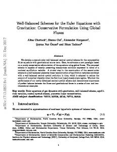
Figure 5. Physical domain for airfoil calculations.

Here, the subscript 1 refers to free-stream values,  is the angle of attack, R and  are the magnitude and angle of the position vector originating from a reference point at the body (i.e., quarter-chord point for airfoil) and extending to the far- eld boundary point, respectively, c is the body length, and cl is the lift coecient. The polar angle  is de ned as positive in the counterclockwise direction relative to a reference line (i.e., coinciding with chord for airfoil) emanating from the leading edge of the body andproceeding downstream. The Cartesianvelocity components u and v of equations (5.3) are used to compute the local tangential and normal velocity components, respectively, required in the boundary conditions. Consider the case of a C-type mesh wrapped around an airfoil, and denote the outer boundary of a nite domain as 61 + 62 ( g. 5). For airfoil computations, the boundary cells at 61 are treated as described in this section. The boundary cells at 62 are also treated in this way when the ow is inviscid. In the viscous ow problem, a portion of the boundary 62 can generally be wake ow. If the boundary conditions applied at 62 for inviscid ows are used for viscous ows, instabilities can occur. One way to treat the boundary cells at 62 is to specify the pressure and extrapolate the variables , u, and v, which would satisfy the requirement of characteristic theory to specify one quantity. However, this approach results inpressure-wave re ections, which can seriously delay the convergence of the numerical scheme. An alternative boundary-point treatment is to extrapolate all dependent variables, allowing the outer and surface boundaries to determine a unique solution. Numerical experiments demonstrate that solutions obtained applying these two treatments are essentially the same near the airfoil. Furthermore, if the outer boundary is far enough away (i.e., 20 chords), there is generally no eect on global quantities such as lift and drag. The second approach shows noticeable improvement in the convergence behavior of the solution algorithm. For internal ows where the inlet Mach number is subsonic, the speci ed ow quantities of equations (5.2) are replaced with the total pressure, total enthalpy, and ow inclination angle. These conditions are usually known for internal ow problems. The Riemann variable R0 is extrapolated from the interior of the domain. At a subcritical exit boundary the pressure is speci ed, while the Riemann variable R+, the total enthalpy, and the velocity component parallel to the boundary are extrapolated from the interior. If supersonic ow occurs at the 30

inlet or exit boundary, the variables at that particular boundary are determined in the same manner described in this section for supersonic external ow problems. 6. Basic Time-Stepping Schemes

In section 6.1, the class of Runge-Kutta (R-K) schemes used for time integration is de ned. The parameters associated with these R-K schemes and the requirements for determining the parameters are discussed. Then, stability analysis for the four-stage and ve-stage schemes that are applied is conducted by considering a linear-wave equation. In section 6.2, stability properties of R-K schemes for systems of uid dynamic equations are presented. This requires writing the Navier-Stokes equations in general curvilinear coordinates and de ning associated Jacobian matrices. With this framework in place, an estimate for the time step is given in section 6.3. 6.1. Ru nge-K utt a Sche mes

For problems where the area of a mesh cell is independent of time, the semidiscrete system of equation (3.2) becomes W + R (W ) = 0 (6 1 1) where R(W ) is the residual function de ned by ) = 1 (L + L + L ) W (6 1 2) R(W d

i ;j

dt

i;j

:

:

:

:

i;j

i;j

C

D

AD

i ;j

i;j

A variety of methods for the integration of ordinary dierential equations (ODE's) can be used to advance the solution of equation (6.1.1) in time. Single-step, multistage schemes (such as R-K schemes) are usually preferred, rather than linear multistep schemes (such as the Adams-Bashforth scheme), because multistep schemes require more storage and introduce implementation diculties when combined with a multigrid method. A four-stage R-K scheme (ref. 1) that belongs to the class of standard R-K schemes and is fourth-order accurate in time is used to solve a system of ODE's corresponding to the Euler equations. The four-stage R-K scheme can be written as 9 (0) = W( ) > W > > > > > > 1 (1) (0) (0) > > W =W 0 2R > > > > > > > > 1 (2) (0) (1) > = W =W 0 2R (6 1 3) > > (3) (0) (2) > > W = W 01 R > > > > >   1 > (4) (0) (0) (1) (2) (3) > W = W 0 6 R + 2R + 2R + R > > > > > > > ; ( +1) (4) W =W n

t

t

:

:

t

t

n

where R( ) = R(W( )), the superscript denotes the time level 1 , and the mesh indices ( ) associated with the solution vector W are suppressed for convenience. If interest is only in steady- ow problems, then the higher order accuracy in time is not important, and other classes of multistage schemes can be considered. Schemes can be constructed with certain desirable q

q

n

n

i; j

31

t

stability and damping characteristics that lead to ecient steady-state solvers. For example, the solution at the (q + 1)th stage (ref. 3) can be expressed as (6: 1:4) W(q +1) = W (0) 0 q +1 1tR (q ) where the residual function ! q q q X X X 1 (r ) (r ) (r ) R(q ) = (6: 1:5)

r =0 qr L C W + r =0 qr LD W + r =0 qr LAD W and the consistency conditions P qr = 1, P qr = 1, and P qr = 1 must be satis ed. The basic parameters p (where p = q + 1 (q = 0; : : : ; m 0 1)) and the weighting factors qr , qr , and qr must be prescribed to de ne the m-stage, time-stepping scheme. The desired stability and damping properties of the scheme provide the requirements for determining the basic parameters and weighting factors. Both hyperbolic and parabolic stability limits must be considered. The hyperbolic and parabolic limits are intervals along the imaginary and negative real axes, respectively, in the complex plane. The coecients p can be chosen to have the best possible hyperbolic or parabolic stability limit without special regard to the high-frequency damping characteristics of the scheme. However, if the scheme is used as a driver of a multigrid method, the scheme must eectively damp the highest frequency error components. Van der Houwen (ref. 39) gives the parameters p that correspond to the maximum (or nearly so) attainable Courant-Friedrichs-Lewy (CFL) number. For schemes with an odd number of stages, Van der Houwen proved that the largest possible stability interval along the imaginary axis of the complex domain is (m 0 1). Vichnevetsky (ref. 40) conjectured that (m 0 1) is also the optimal CFL number when m is even, and demonstrated this concept for m = 2 and 4. Sonneveld and Van Leer (ref. 41) proved that the (m 0 1) CFL number limit is valid when m is even. Jameson (refs. 3 and 42) considers schemes with the p 's of Van der Houwen, and de nes appropriate weighting factors for the arti cial dissipation evaluations to yield a good parabolic limit. Although the p 's are obtained using only a hyperbolic stability limitation, they are still a good choice for a viscous ow solver, especially at high Reynolds numbers. That is, the convection (hyperbolic) limit on the time step remains the controlling stability factor for practical aerodynamic ows. Several members of the class of schemes de ned by equations (6.1.4) and (6.1.5) have been analyzed in reference 42 by considering the model problem @ 4w @w @w + a + 4 1x3 4 @t @x @x

=0

(6: 1:6)

Equation (6.1.6) is the 1-D, linear-wave equation with a constant-coecient, third-order dissipation term. If the spatial derivatives in equation (6.1.6) are approximated with central dierencing, then = 0 N2 (wnj+1 0 wjn01) 0 4 Na (wjn+2 0 4wjn+1 + 6wjn 0 4wjn01 + wjn02) 1t dw dt

(6: 1:7)

where N = a 1 t=1x is the Courant number. Taking the Fourier transform of equation (6.1.7), obtain (6: 1:8) 1t ddtw^ = z w^ n where the Fourier symbol N z = 0 iN sin  0 44 (1 0 cos )2 (6: 1:9) a 32

Here, i =

p0 1, and  is the Fourier angle. If the residual function for any stage q is given by R(q ) = (L C + LAD ) w(q )

(6: 1:10)

then the ampli cation factor for an m-stage scheme is

g(z) = 1 + ^f ()z ()

(6: 1:11)

where

f^ () = 1 + 2z2 + 1 1 1 + mzm (6: 1:12) Here, 1 = m with m = 1 for consistency, and l = l 01 m0 l+1 with l = 2; 3; : : : ; m. Since g(z) is analytic, the maximum modulus theorem guarantees that all contours jg (z)j < 1 lie inside the absolute stability curve jg (z)j = 1. For this subclass of schemes, which are schemes satisfying the requirement that jzj  (m 0 1) (refs. 3 and 41), the optimal polynomials are de ned as

 0 iz  ik   0 iz   0 iz  + Tk 0 Tk 0 2 k 01 2 k01 k 01 polynomial, and k  2. The coecients l for the

g(z) = Pk (z) = ik 0 1Tk 0 1

where Tk is a Chebyshev ve-stage schemes given in reference 39 are

(6: 1:13) four-stage and

1 = 1 1 2 1 3 = 6 1 4 = 24

2 =

and

1 = 1 1 2 3 3 = 16 1 4 = 32 1 5 = 128

2 =

respectively.

In the more general situation, the ampli cation factor is not a polynomial in z. For example, consider the subclass of schemes de ned by equation (6.1.5) that are called (m; n) schemes. The m refers to the number of stages, and n designates the number of evaluations of the dissipative contribution. For example, assume a (m; 2) scheme, where the numerical dissipation terms are evaluated on the rst and second stages and frozen for the remaining stages (similar to the (4; 2) scheme used). Let zr = > > > > > > > > > > > > > > > > >

30 = 03 > > > =

31 = 0 >

32 = 3 > > > >

33 = 0 > > >

40 = 0305 > > >

41 = 0 > > >

42 = 3 05 > > >

43 = 0 > > > ;

= >

00 = 1

10 = 1

11 = 0

20 = 03

21 = 0

22 = 3

44

(6:1:15)

5

where 03 = (1 0 3), 05 = (1 0 5), 3 = 0:56, and 5 = 0:44. The symbol of the time-stepping operator ^f for this scheme is given by

h

f^ = 5 1 0 4 z1 (1 0 3 zi ) 0 4z3z1 (3 z2 zi 0 3 zr ) 0 05 3 z3 zr where

z1 = zi + 5zr z2 = zi + 3zr

z3 = 2(1 0 1 zi ) 34

i

(6:1:16)

In a number of ow computations, four-stage and ve-stage schemes are applied (refs. 19, 24, 43, and 44). For these schemes, the residual function is q X 1 ( q ) ( q ) (0) (r ) R =

L C W + LD W + r =0 qr LAD W

!

(6: 1:17)

By evaluating the physical diusion terms on the rst stage only, the computational eort of the scheme is reduced. This incompatibility with the computation of the numerical dissipation terms does not cause any deterioration in the performance of the schemes. The evaluation of the numerical dissipation terms on certain stages (and the weighting of these evaluations) provides two advantages. First, the parabolic stability limit can be extended, and the high-frequency damping can be improved. Second, the expense of calculating the dissipation terms can be reduced. Reference 3 provides additional discussion on the weighting of dissipation. The time-stepping parameters for the four-stage scheme are 9 1 1 = > > 4> > > > 1 2 = = 3 (6: 1:18) > > 1 3 = > > 2> > > ; 4 = 1 Since m01 = 1=2, the scheme is second-order accurate in time. The numerical dissipation terms are evaluated the same as for equation (6.1.14). For the model problem of equation (6.1.6), the absolute stability curve for this scheme is presented in gure 6(a). The hyperbolic pstability limit (as determined by the extent of the stability interval on the imaginary axis) is 2 2. The parabolic stability limit (as determined by the extent of the stability interval on the negative real axis) is 4. The dashed line ( g. 6(a)) represents the locus of the Fourier symbol as de ned in equation (6.1.9), and must lie inside the j gj = 1 curve for stability. Figure 6(b) shows the variation of the ampli cation factor g with the Fourier angle . The scheme exhibits good high-frequency damping, which is crucial for a rapidly convergent multigrid method. When analyzing the stability and damping properties, it is important to include all components of the scheme. For example, if the stability limit of the algorithm is extended through the introduction of an implicit residual smoothing procedure (discussed in section 7.2), some deterioration in the high-frequency damping occurs ( gs. 6(c) and 6(d)). In the case of the ve-stage scheme, the basic parameters are

9 1 1 = > > 4> > > > 1 2 = > > 6> > = 3 3 = > 8> > > > 1 > 4 = > 2> > > ; 5 = 1 35

(6: 1:19)

3

1.0

2

.8

1

.6 g

y 0

.4 –1 .2 –2 –3 –6

–5

–4

–3

–2 x

–1

0

1

0

2

(a) Stability curves with two evaluations of dissipation; CFL = 2.4; (2) = 0; (4) = 1=32.

.5

1.0

1.5

θ

2.0

2.5

3.0

3.5

(b) Amplication factor with two evaluations of dissipation; CFL = 2.4; (2) = 0; (4) = 1=32. 1.0

3 2

.8

1 .6 g

y 0

.4 –1 .2

–2 –3 –6

–5

–4

–3

–2 x

–1

0

1

0

2

(c) Stability curves with implicit residual smoothing; CFL = 4.8; = 0:6; (2) = 0; (4) = 1=32.

.5

1.0

1.5

θ

2.0

2.5

3.0

3.5

(d) Ampli cation factor with implicit residual smoothing; CFL = 4.8; = 0:6.

Figure 6. Plots of four-stage R-K scheme; (2) = 0; (4) = 1=32; coecients are 1/4, 1/3, 1/2, and 1.

36

A very large parabolic stability limit is established by evaluating the arti cial dissipation terms on the rst, third, and fth stages with the weightings of equations (6.1.15). Figure 7(a) shows that for this scheme, the hyperbolic stability limit is 4 and the parabolic stability limit is about 9. Figure 7(b) shows that this ve-stage scheme also has good high-frequency damping. Figures 7(c) and 7(d) show the stability curves for this scheme when implicit residual smoothing is applied. In practice, with the implicit residual smoothing, a CFL number of 7.5 is used for this scheme. For the four-stage scheme, a CFL number of 5.0 is used. So, with one additional evaluation of the implicitly smoothed residual function, the CFL number increases by a factor of 1.5.

1.0

4 3

.8 2 1

.6 g

y 0

.4

–1 –2

.2

–3 –4 –10 –9 –8 –7 –6 –5 –4 –3 –2 –1 0 1 x (a) Stability curves with three evaluations of dissipation; CFL = 3.0.

0

.5

1.0

1.5

θ

2.0

2.5

3.0

3.5

(b) Ampli cation factor with three evaluations of dissipation; CFL = 3.0. 1.0

4 3

.8 2 1

.6 g

y 0

.4

–1 –2

.2

–3 –4 –10 –9 –8 –7 –6 –5 –4 –3 –2 –1 0 1 x (c) Stability curves with implicit residual smoothing; CFL = 6.0; = 0:6.

0

.5

1.0

1.5

2.0 2.5 3.0 3.5 θ (d) Ampli cation factor with implicit residual smoothing; CFL = 6.0; = 0:6.

Figure 7. Plots of ve-stage R-K scheme; (2) = 0; (4) = 1=32; coecients are 1/4, 1/6, 3/8, 1/2, and 1.

37

6.2. S tab ility of R unge- Ku tta S ch emes for Sys tems

The compressible Navier-Stokes equations can be classi ed as either hyperbolic-parabolic or incomplete-parabolic type (refs. 45{47). As discussed in section 6.1, these equations are solved numerically with a member of a class of multistage time-stepping schemes. By considering the hyperbolic (inviscid) and parabolic (viscous and numerical dissipation) operators separately, sucient conditions for stability can be obtained. These conditions can be used as a starting point for estimating a time step for solving the full Navier-Stokes equations. To estimate the restriction on the time step due to convection and diusion, we consider the two-dimensional, Navier-Stokes equations expressed in generalized coordinates (; ). These equations can be written as e( ) f @F @W + @t @

e ()

e ( )

e ()

+ @ F@ = @ F@ v + @ F@v

(6: 2:1)

f = J 01 W , with J 01 and W representing the inverse of the transformation Jacobian where W and the vector of conserved ow variables, respectively. The derivatives associated with the transformation from Cartesian coordinates (x; y) to (; ) and the corresponding inverse transformation are related as     y 0y  x x = 1

y y

J 01

0 x

x

and the inverse of the transformation Jacobian is given by @ (x; y) = x y 0 x y =

J 01 = @ (; ) The transformed inviscid ux vectors F~ ( ) and F~ () are given by ( ) = J 01 (xF( ) 0 y F())

(6: 2:2)

() = J 01 (xF() 0 yF() )

(6: 2:3)

e F e F

Using the notation of reference 48, the viscous ux vectors Fe v( ) and Fev( ) can be expressed as f f ( ) = B e (; ) @ W + B e (;) @ W @ @

(6: 2:4)

f f () = B e (; ) @ W e (; ) @ W + B @ @

(6: 2:5)

ev F ev F

where

e (; ) = B (; ) M; B 1

; 2 f;  g

38

(6: 2:6)

e v vectors in terms of primitive and B1 is a viscous matrix obtained by rewriting the F variables. The matrix M , which transforms nonconservative (primitive) variables to conservative variables, and the inverse of matrix M are given by (; )

2 1 66 0u 01 M=6 64 0 v01 2

2 66 0 1 M =6 64

and

0

0 0

0 1 0 0 ( 0 1)u 1

0 0

 01 0 0 ( 0 1)v ( 0 1) 0

0

0

3 77 77 5

(6: 2:7)

3 77 77 5

u  0 0 (6: 2:8) v 0  0 ( 0 1)0 12 u v ( 0 1)0 1 e (;) , Be (;), Be (; ), and Be (;) respectively, with 2 = ( 0 1)(u2 + v 2)=2. The viscous matrices B are de ned according to

2 66 Be (; ) = 6 66 4

0

0

0

0 0

; B; Bx;x x;y ; 0 By;x B; 0 y;y ; u + B ; v B; v + B ; u B; 0 1 0B ; p02 Bx;x y;x y;y x;y

with ; = Ba;b

B ; =

0

3 77 77 75

 p M  @ @ @ @  + +  r 1 r  Re

@a @b

@b @a

(6: 2:9)

(6: 2:10)

a;b

p M    r 1 r Re 0 1 P r

(6: 2:11)

where the nondimensionalization of section 3.1 is employed, r is the gradient operator, and e () = @ Fe () =@W f , where  2 f; g, a;b is the Kronecker delta. Using the Jacobian matrices A equation (6.2.1) can be rewritten as

f e () @ W f @ e (;) @ W f e (; ) @ W f f e () @ W @W +A +A = B +B @t @ @ @ @ @

!

f e (;) @ W f @ e (;) @ W + B +B @ @ @

! (6: 2:12)

where

2 3 y 0 0 x 66 0 uU () +   2 U () 0 ( 0 2) u  u 0 ( 0 1) v ( 0 1) 77 x x y x x7 (  ) e = 66 A 64 0 vU () +  y 2  xv 0 ( 0 1) yu U ( ) 0 ( 0 2) y v ( 0 1) y 775 U () ( 2 0 !)  x! 0 ( 0 1)uU () y ! 0 ( 0 1)vU ()

U ( ) 39

(6: 2:13)

with U () =  xu +  y v, and ! = E 0 2 . Assume the coecient matrices of equation (6.2.12) are locally constant in space and time, and transform to primitive variables. Then, obtain @W @W @ 2W @ 2W @ WP + A ( ) P + A () P = B (; ) 2 P + B (;) 2 P @t @ @ @ @  2  (;) @ WP + B + B (; ) @ @

where

(6: 2:14)

WP = [  u v p ] T

(6: 2:15)

3 2 ( )  x  y 0 U 6 ( ) 01 x 7 7 6 0 0  U ( ) 7 6 e ( )M0 1 = 6 A = MA ( )  01  y 7 7 6 0 0 U 5 4 (  ) 0 p x py U

(6: 2:16)

2 6 6 B (; ) = MB1( ; ) =  01 6 6 6 4

0 0

0

0 0 ( 0 1)B ; p01

0

 ; B; x;x Bx;y  ; B; y;x By;y

0

0

0 0 0 ( 0 1)B;

3 7 7 7 7 7 5

(6: 2:17)

The eigenvalues of the matrices A ( ) are 9 > > > > > > > > =

U ( ) U ( )

q U ( ) + c x2 + 2y > > > > > > q > > (  ) 2 2 U 0 c x + y ;

(6: 2:18)

The eigenvalues of the matrices B ( ; ) are 0

 0 Pr 1

01

(2  + )01 where 01 =

p M 1

9 > > > > > > = > > > > > > ;

(2 + 2y ) Re  x 40

(6: 2:19)

For the matrices B (; ), the eigenvalues are 0

9 > > > > > > > > > > > > =

p M    2 Pr  (r 1 r ) Re  p M  ( + 3 ) (  + ) > (r  1 r ) +  jrj jr j > > > Re  > > > >   p M ( + 3 ) > > (  + ) > ; ( r  1 r ) 0 jr  j jr j > Re  

(6: 2:20)

Abarbanel and Gottlieb (ref. 49) showed that the matrices of equation (6.2.14) can be simultaneously symmetrized with the similarity transformation determined by 2p 6 6 S=6 6 6 4

c0 1

0 1 0 0

0 0

p1 c

2 p1 01 0 1

 c 6 6 0 6 S 01 = 6 6 0 4 0 p 1 c

(

0 1)

0 0 1 0 0 1 0 0

3

0 0 0

p 0 1 p c

0 0 1 0

7 7 7 7 7 5

0 0 0

p p 0 1 0 1 c0 1

(6: 2:21)

3 7 7 7 7 7 5

(6: 2:22)

Using this similarity transformation, rewrite equation (6.2.14) as  @2V @V @V @2V @2V  @V + A( ) + A() = B (; ) 2 + B(; ) 2 + B (; ) + B (;) @t @ @ @ @ @@ 

where

9 A( ) = S 01 A ( ) S = ; B (; ) = S 01 B ( ; )S

(6: 2:23) (6: 2:24)

with ; 2 f; g. De ne as a discrete computational domain f(; ) : 1    L, 1    L, and1  = 1 = 1g, where L = N, the number of mesh intervals in either coordinate direction. Let a discrete, vector function, such as V(i 1;j 1) = V(i;j ), be denoted by Vi;j . If the spatial derivatives of equation (6.2.23) are approximated with second-order central dierences, the semidiscrete representation d (6: 2:25) V + L Vi;j = 0 dt i;j 41

is obtained, where LVi;j = (A( ))i;j   Vi ;j + (A() )i;j   Vi;j 0 (B (; ))i;j 2 Vi ;j i h 0 (B ( ;))i;j + (B (; ))i;j      Vi ;j 0 (B (;) )i ;j 2Vi;j

(6: 2:26)

Then, taking the Fourier transform of equation (6.2.25) yields 1t ddt V^ i;j = 01t L^ V^ i ;j = Z V^ i;j where the caret indicates a transformed quantity, and Z = ZC + ZD with  ( ) sin  + A( ) sin   Z C = 0 i 1t A ZD

p

= 0 1t

(6: 2:27)



4 B( ; ) sin2  + (B ( ;) + B( ; ) )sin  sin  + 4B( ; ) sin2  2



2

and i = 01. If all terms in the ow equations and the numerical dissipation are evaluated at each step of the R-K scheme, then the ampli cation matrix G for an m-stage scheme is a function of one variable. In particular 2 m G(Z ) = I + 1Z + 2 Z + 1 1 1 + m Z (6: 2:28) where 1 is a function of the coecients of the R-K scheme. (See eq. (6.1.12) for de nition.) Let ^ ) be any eigenvalue of L^ . Also, let z = 0 1tq (L^ ). q (G) be any eigenvalue of G(Z ), and let  q (L The eigenvalue q (G) is related to z as ( ) = 1 + 1z + 2 z2 + 1 1 1 + m zm

q G

(6: 2:29)

The stability of a scheme requires that the ampli cation matrix satis es the condition n k  C for all n. The spectral radius  of a matrix is de ned as equal to the largest eigenvalue in absolute value. If the matrix G is normal (i.e., GG3 = G3 G), then its norm is equivalentto the spectral radius (G). Thus, a normal matrix requires that (Gn ) = n(G)  C: This condition is equivalent to the Von Neumann condition for stability that requires (G)  1 (6: 2:30) Hence, if Z and G are normal matrices, the condition for stability is   (6: 2:31) j g(z )j = jg 01t q (L^ ) j  1 k

G

for all q . To determine sucient conditions for stability, consider separately the hyperbolic and parabolic operators associated with equation (6.2.1). First examine the stability for the Euler equations (i.e., Re ! 1 in eq. (6.2.1)). The following theorem gives a sucient condition for stability: 42

The orem 6.1

Suppose the R-K scheme satis es the property that

[0 i NCFL ; i NCF L]  fz 2 C : j g(z )j  1g

(6: 2:32)

where NCF L is the CF L number for the R-K scheme. Assume smooth initial data, such that the Cauchy problem for the Euler equations is well-posed. If the Euler equations are solved with this R-K scheme and second-order centered dierence approximations for the spatial derivatives, the condition

1 t [ (A( ) + A())]  NCF L where jj

(6: 2:33)

 1, and j j  1 is sucient for stability of the linearized problem.

The proof follows directly. Since the matrices A() and A() are symmetric, the ampli cation matrix G(Z ) is normal. Furthermore, for a central dierence scheme, the Fourier transform of the rst derivative is a pure imaginary number. Hence, Z = 0i 1t A( ) sin  + A() sin  , and so the result follows (remember that 1 = 1 = 1). Now consider the parabolic equation derived from equation (6.2.23) by eliminating the rst-order spatial derivatives. The Fourier symbol of the dierence operator is given by equation (6.2.27) when A()  0. Let ND denote the diusion number of the R-K scheme (i.e., ND de nes the stability interval along the negative real axis). Then, the maximum allowable time step is ND 1tD , where 1tD = 1x2 =(4) for the 1-D scalar diusion equation with central dierencing, with  being the diusion coecient. A sucient condition for stability is de ned as follows: The orem 6.2

Suppose the R-K scheme satis es the property that

[0ND ; 0]  fz 2 C : j g(z)j  1g

(6: 2:34)

where ND is the diusion number for the R-K scheme. Assume smooth initial data, such that the Cauchy problem for the viscous equations is well-posed. If the viscous equations are solved with this R-K scheme and second-order centered spatial dierencing, the condition

max(1t D )  ND with

D

(6: 2:35)

   = 4  B (;) sin2 2 + B (;)sin2 2 + 14 (B (; ) + B (;) )sin  sin 

is sucient for stability of the linearized equation.

Since

Z = 01 t

 

4

 B (;) sin2 

+ B (;)sin2 



+ (B (;) + B (; ))sin  sin 



(6: 2:36) 2 2 is a negative real symmetric matrix, G(Z ) is again normal. Therefore, the proof is similar to the proof of theorem 6.1. Note that if the cross-derivative terms are neglected, the inequality of equation (6.2.35) reduces to i h  1t 4  B (; ) + B (;)  ND 43

(6: 2:37)

Next, suppose numerical dissipation in the form of fourth-dierence terms is added to the discrete viscous equations. Then LVi;j = 0 (B ( ; ))i;j  2 Vi;j 0 (B (;))i ;j 2 Vi;j h

0 (B( ;) )i ;j + (B (; ))i;j

i

    Vi ;j

+ "(4)(A~ ( ))4Vi;j + "(4) (A~( ))4 Vi;j (6: 2:38) and the Fourier symbol of equation (6.2.27) is replaced by Z = ZD + ZAD , where ZD is de ned the same as in equation (6.2.27), and 

Z AD

 = 0 161t "(4) Ae () sin4 

2

+ Ae () sin4 



2

I

with I being the identity matrix.

If only the viscous terms and the fourth-dierence dissipation terms are considered, then the condition Le mma 6.3

max [1t (D + AD )]  ND

with D the same as given in equation (6.2.35) and   (4) e ( ) sin4  AD = 16 "  A

2

(6: 2:39)

+ Ae( ) sin4 



2

is sucient for the linearized stability of the multistage scheme.

The proof is the same as the proof for theorem 6.2. If cross-derivative terms are neglected, the inequality of equation (6.2.39) becomes h   i  1t 4  B ( ; ) + B (;) + 16 "(4)  Ae ( ) + Ae ( )  ND (6: 2:40) 6.3. Time S tep Es timate

Now consider the situation where the R-K scheme simultaneously satis es the properties of equations (6.2.32) and (6.2.34). Also consider the 1-D  case in the  direction. The R-K scheme then depends on the matrix Z , where Z = 0 1t iA ( ) sin  + 4B ( ; ) sin2  =2 . Since A() and B (; ) do not commute, the matrix Z , and thus the ampli cation matrix G, are no longer normal matrices. Hence, the Von Neumann condition on the largest eigenvalue of matrix G is now a necessary, but not a sucient, condition for stability. Thus, there is no simple way to go from properties of matrix Z to properties of matrix G. The spectral mapping theorem relates the eigenvalues of matrix Z to the eigenvalues of matrix G. Since the eigenvalues do not tell the entire stability story, energy estimates based on norms must be used. However, no simple relationship exists between the norm of matrix Z and the norm of matrix G. In practice, a simpli ed stability condition is used to estimate the time step. There is no strict mathematical proof of stability with this condition; nevertheless, it seems to work well. Consider 1tC = NCF L C

1tD = N D D

44

where Let so that

= (Ae ( )) + (Ae () ) e (; ) )+ (Be (;) )+  (Be (;)) D = (B 1 = 1 + 1 1t 1t C 1 tD C

(6: 3:1) 1t =  + (NNC F L=N ) C CF L D D Schemes in which NCFL  ND have been considered. The time step for each cell in the computational domain is then computed as (6: 3:2) 1t = NCF+L

C D where is the cell area and C =  +  D = (D ) + (D ) + (D ) with  and  de ned by equation (4.2.5), and p M  9 01 (x2 + y 2) >

( D ) = Re   > P r > > p M  = (D ) = Re P r 01 (x2 + y2 ) (6: 3:3) > > p M 1 h q 2 2 2 2 i> > (D ) = Re  0( + 3)(y y + x x )+ ( + ) (y + x)(y + x ) ; For the thin-layer, Navier-Stokes equations, take D = (D ) , where  is the direction normal to the boundary layer.

So far, only central dierencing is considered for the spatial approximations in estimating a time step for an explicit R-K scheme. Since a numerical- ux function for an upwind scheme can generally be expressed as the sum of a centered (physical) contribution and a numerical dissipation contribution, then equation (6.3.1) is also a reasonable estimate for the time step when an upwind scheme is used. Re mark 6.4

7. Convergence Acceleratio n Tech niques 7.1. Local T ime Step ping

The rst technique employed to accelerate convergence of the basic explicit time-stepping scheme to a steady-state solution is local time stepping, where each cell is updated using an individual time step. For simplicity, the one-dimensional Euler equations are used to understand the meaning of local time stepping from the discrete point of view. Suppose the Euler equations are written in the form @W @W + A =0 @t @x If the equations are discretized in an explicit sense, then f = Ae W fn 1W 45

where the tilde indicates that the vector or matrix is for the complete discrete system. The block matrix Ae is a function of 1t min=1x, with 1tmin being the minimum time step permitted in the domain, and each element of Ae being a 3 by 3 matrix. Let the explicit matrix Ae for the system of dierence equations be preconditioned by the diagonal matrix 3, given by 2 3 3 = Diag 1t 2I 1t3 I 1 1 1 1tN 02I 1tN 01 I where 1ti = 11t t i i=2 N 01 min Here, 1ti is the largest local time step allowed by stability, and I is a 3 by 3 identity matrix. This process results in a signi cant speedup in the transport of information, and an increase by roughly a factor of two in the convergence rate of explicit schemes. 7.2. Res id ua l S moothing

The local stability range of the basic time-stepping scheme can be extended by applying a procedure called implicit residual smoothing. This technique was rst introduced by Lerat (ref. 50) for the Lax-Wendro scheme, and later devised by Jameson (ref. 51) for R-K schemes. The constant-coecient approach of Jamesonis discussed in section 7.2.1. Some basic properties of residual smoothing are also presented. Then, variable coecients for implicit smoothing are discussed. The coecients introduced in this paper, and those of Martinelli (ref. 27), are derived and compared. In section 7.2.3, coecients are developed for implicit residual smoothing that allow a time-step estimate independent of a physical diusion limit.

7.2.1. Constant coecients. The constant-coecient, implicit residual averaging of Jameson (ref. 51) can be applied in two dimensions using the factored form (1 0  r 1 )(1 0  r 1 )Ri;j(m) = R(i;jm)i

(7: 2:1)

where the quantity r 1 is a standard second-dierence operator, and thus r  1 R i;j(m) = Ri(0m1);j 0 2Ri;j(m) + Ri(+1m;j)

The quantity is a smoothing coecient, and (; ) are the coordinates of a uniformly spaced, computational domain. The residual of the unsmoothed scheme R(i;jm) is de ned by (m01) + L W(0) + AD (m) ] R(i;jm) = m 1 ti;j [L C Wi;j D i;j i;j

(m = 1; 5)

(7: 2:2)

and computed in the Runge-Kutta stage m, AD (m) is the total arti cial dissipation at stage m, and Ri;j(m) is the nal residual at stage m after the sequence of smoothings in the  and  directions. A tridiagonal system of equations is solved for each coordinate direction to obtain the unknown residuals Ri;j(m). To determine  and  , Jameson (ref. 51) considers the model problem of equation (6.1.6) without numerical dissipation (i.e., the convection equation). Then, the semidiscrete equation (6.1.7) becomes 1t dw = 01t Lwj dt 46

with

1t Lwj = N2 (wjn+1 0 wjn01 ) and the Fourier symbol of the dierence operator 01t L is given by z = 0 1tL^ = 0iN sin  (7: 2:3) Let 1wj de ne the correction, or residual, obtained from the implicit smoothing procedure, so that (7: 2:4) (1 0 r1) 1wj = 1wj and the Fourier symbol of equation (7.2.3) is replaced by N sin  (7: 2:5) z = 0i 1 + 4 sin2 2 A sucient condition for stability is as follows: max jzj  N 3 (7: 2:6) for all , and N 3 is the Courant number of the unsmoothed scheme. Solving for sin  and cos  corresponding to the maximum of jz j yields p 9 1+ 4 > sin  = 1+ 2 > > = (7: 2:7) > 2 > cos  = 1+ 2 ; Using equations (7.2.7) and the sucient condition of equation (7.2.6), the smoothing coecient is determined by " 2 # N 1 (7: 2:8a)  4 N3 0 1 or " 2 # 1 1t 0 1  (7: 2:8b) 4 1t 3 where 1t 3 is the time step of the unsmoothed scheme. In subsequent discussion, this will be referred to as the 1-D smoothing coecient and will be designated by 10D. Instead, consider the diusion equation @w @ 2w =  2 @t @x

If the spatial derivative is again approximated with a central dierence, and a Fourier transform is taken of the resulting semidiscrete equation, the Fourier symbol of the product of 1t and the dierence operator are given by  z = 0 ND sin2 2 2 where the diusion number ND = 41t=1x . If the residual smoothing operator of equation (7.2.4) is applied, then 0 ND sin2 =2 z= (7: 2:9) 1 + 4 D sin2 =2 47

A sucient stability condition for an R-K scheme is max jzj  ND3 for all , where ND3 is the diusion number of the unsmoothed scheme. With the same procedure employed for the convection equation, the smoothing coecient is determined as 1  ND 0 1 = 1  1t D 0 1 D  (7: 2:10) 4 ND3 4 1t 3D Thus, for the scalar diusion equation, the smoothing coecient D is proportional to  1t=(1x)2 . As will be shown in section 7.2.3, this type of can be combined with the type of given by equations (7.2.8) to yield a formulation suitable for a convection-diusion equation. Some properties of implicit residual smoothing are now examined. If residual smoothing is applied on each stage of an R-K scheme, the stability function given in equation (6.1.11) still applies, with the z of the original (basic) scheme modi ed as in equation (7.2.5) or (7.2.9). This stability behavior leads to the following theorem: ^ be the Fourier symbol of any discrete spatial operator for the convectionThe orem 7.1 Let L

diusion equation. Let equation (6.1.11) be the stability polynomial for an explicit m-stage R-K scheme. Apply implicit residual smoothing, as in equation (7.2.4), after every stage of the R-K scheme.

If the original scheme is unconditionally unstable, then the smoothed scheme is also unconditionally unstable. If the original scheme is conditionally stable, then the smoothed scheme can be made unconditionally stable by choosing 1t suciently large. Pro of.

Let z and zs be the symbols of the original and smoothed schemes, respectively. Then, z

(7: 2:11) 1 + 4 sin2 =2 De ne r as the position vector corresponding to z. Thus, r emanates from the origin of the complex domain and has magnitude j zj. Let rs be the position vector associated with zs. If the original R-K scheme is stable, then r does not terminate outside the stability region S , determined by the Von Neumann condition jg(z)j  1, where g(z) is the stability polynomial. If the original scheme is unstable, then there is no 1t > 0 small enough to allow r to be in S . Since the denominator of equation (7.2.11) merely acts as a scaling factor of r, the residual smoothing cannot stabilize the unstable original scheme. Suppose is proportional to 1t, as in equations (7.2.8) or (7.2.10). Then, rs does not terminate outside the boundary of S for any value of 1t , since can always be made suciently large. Moreover, the scheme is unconditionally stable. zs =

Even though the explicit R-K scheme can be made unconditionally stable with the implicit residual smoothing, there is a practical limit on the time step when solving the hyperbolic problem and taking / 1t 2, as in equations (7.2.8). That is, if 1t is too large, convergence slows down. Re mark 7.2

Le mma 7.3

equation

Apply an explicit m-stage R-K scheme with implicit residual smoothing to the scalar @4w @w + "(4)1x3 4 = 0 @t @x 48

(7: 2:12)

where "(4) is a constant coecient. Assume that the residual smoothing coecient is proportional to N 2. Then, the symbol of the smoothed scheme vanishes as 1t ! 1 and the stability polynomial g(z ) ! 1. The symbol for the dierence operator of equation (7.2.12) when implicit residual smoothing is applied is given by 016"(4)N sin4 =2 zs = 1 + 4 sin2 =2 Using  N 2 and taking 1t to be large, then  4 zs  0 "(4) sin2 N 2 Therefore, zs ! 0 as 1t ! 1. From equation (6.1.11), it follows immediately that g(z) ! 1 as zs ! 0. Pro of.

As evident from Lemma 7.3, the limit on the extension of stability with the implicit smoothing and equations (7.2.8) is caused by the requirement to have a certain background dissipation (i.e., high-frequency damping). If  N , as in the parabolic problem, then the symbol zs does not vanish. Re mark

The use of constant coecients in the implicit treatment (eqs. (7.2.8)) proves satisfactory (extending the Courant number by a factor of two to three) even for highly stretched meshes of viscous- ow computations (ref. 16), provided additional support such as enthalpy damping (ref. 1) is introduced. However, the use of enthalpy damping, which assumes constant total enthalpy throughout the ow eld, precludes the solution of problems with heat-transfer eects. By using variable coecients  and  , which account for the variation in mesh-cell-aspect ratio, residual smoothing can be applied without the support of enthalpy damping.

7.2.2. Variable coecients. The alternating direction implicit (ADI) scheme and the implicit scheme of Lerat (ref. 52) exhibit a functional dependence of variable smoothing coecients on the characteristic speeds  and  , as de ned in section 4.2 of this report. Appendix B shows this functional dependence. Then, with a 2-D stability analysis similar to the 1-D analysis of the previous section, variable smoothing coecients can be obtained as ( " 2 # ) 9 > 1 N 1 >  = max > 4 N 3 1 + r  0 1 ; 0 > = 8 2 3 9 (7: 2:13) ! 2 > > 5 4  = max 0 1 0 1 ; 0; > ; : 4 N 3 1 + r where again r =  = i. The limiting cases are  ! 10D;  ! 0 as r ! 0 and ! 0;  ! 10D, as r  ! 1. A problem exists with the smoothing coecients of equations (7.2.13). In the typical case of N=N 3 = 2, the smoothing coecients vanish when r = 1, making the scheme unstable.



49

Martinelli (ref. 27) eliminates this diculty by modifying the residual smoothing coecients of equations (7.2.13) as follows: ( "

1  = max 4

8 2 > > > =

(7: 2:14)

3 9> => 0 15 ; 0; > > ;

(7: 2:15) and the exponent  is taken to be 2=3. The function  is the same function used for scaling the arti cial dissipation coecients. The introduction of this function seems appropriate because of the direct relationship between residual smoothing and arti cial dissipation. For example, a desired high-frequency, damping behavior of the scheme can be maintained when the dissipation is increased by increasing the residual smoothing. The variable smoothing coecients  and  of equations (7.2.14) cannot be uniquely determined from a sucient condition for stability, as the constant coecient was in equations (7.2.8). Wigton and Swanson (ref. 53) use an additional constraint to derive the parameters of equations (7.2.14). For completeness the short derivation of reference 53 is presented. Consider the following sucient condition for stability: 1 p 1 + N 1 p 1 1 N (7: 2:16) 3 N 1 + r  1+ 4  N 3 1 + r 01 1 + 4   (r ) = 1+ r 

as derived in appendix B. Let the Courant numbers for the two coordinate directions  and  be given by 9  1 tact N > N = > 1t  = N  +  = 1 + r  > = (7: 2:17) 1 tact  N > > N = ; 1t = N  +  = 1 + r 01 > where 1tact is the 2-D allowable time step for convection, and1t  and 1t are the corresponding 1-D time steps. If the Courant number N in equation (7.2.16) is replaced according to equations (7.2.17), the result is N p 1 + N p 1 1 (7: 2:18) N 3 1 + 4  N 3 1+ 4  As suggested by lemma 7.3,  and  should be as small as possible and still maintain stability. With this objective in mind,  +  is minimized subject to equality in equation (7.2.18). Apply the method of Lagrange multipliers and consider the function N F (  ;  ) =  +  + ! N3

 p1 +1 4 + N p 1+1 4 3 N  

50

!

After equating the partial derivatives of F (  ;  ), with respect to  and , to zero, obtain

N

Now, solving for

p1 + 4



1 1 = N 3=2 (1 + 4  ) (1 + 4  )3=2

(7:2:19)

and substituting the resulting expression into equation (7.2.16) yields

N 1 N 3 1 + r

"

  1 + r  N 01=3 1 p1 + 4 1 + 01 N 1 + r 

#

1

(7:2:20)

With the equality of equation (7.2.20) holding, and using equations (7.2.17), obtain the smoothing coecients of equations (7.2.14). As shown in reference 53, the function  arises without any consideration of numerical dissipation terms. The role of the  function is to connect the values of corresponding to low-aspect-ratio and high-aspect-ratio cells. The variation of  from equations (7.2.14) with r is shown as a solid line in gure 8(a). For this curve, the ratio of Courant numbers N=N 3 is assumed to be 2. Observe that  ! 10D for r ! 0, and  ! 0 for r  ! 1. In the case of r = 1,  =  = 10D (a value of 0.75 when N=N 3 = 2). Based upon numerical calculations for inviscid ows using typical inviscid meshes, smoothing coecients  and  that are constant with a value of about 0.4 result in rapid convergence. Values for   0:75 and/or   0:75 can cause a signi cant slowdown in convergence. To provide improved smoothing coecients, when r  1 the formulas of equations (7.2.14) can be replaced with

( " 1 N

# ) 9 > > 0 1 ;0 >  = max 3 > 4 N 1 + r > = 8 2 3 9 !2 > 1 > 5 4  = max 0 1 ; 0 ; : 4 N 3 1 + r 01 ;> 1

2

(7:2:21)

where is a parameter to be speci ed. Here, the connection function  is removed by introducing . Figure 8(a) shows the curve representing  when N=N 3 = 2 and = 0:25. For the case of r = 1,  is 0.39. 51

1.2

Martinelli (ref. 27) Swanson (ref. 44)

1.0

.8

βξ .6

.4

.2

0 10–3

10–2

10–1

100

101

102

rηξ

(a) Variation of coecient  with mesh cell aspect ratio r  . 2 Martinelli (ref. 27) Swanson (ref. 44)

0 –2 –4 Log, –6 residual –8 –10 –12 –14 0

50

100

150

200

250 300 Cycles

350

400

450

500

(b) Residual histories. RAE 2822 airfoil, M1 = 0:75,  = 3 , 224 by 32 grid. Figure 8. Implicit residual smoothing coecient for two forms of variable coecients. 52

To investigate stability using the smoothing coecients of equations (7.2.21), consider the sucient stability condition sin  N N 1 1 sin  + 3 3 0 1 N 1 + r   N 1 + r  

1

(7:2:22)

for all  and  . In equation (7.2.22) 19

0

 = 1 + 2  1 0 cos  =

(7:2:23)

0 1  = 1 + 2  1 0 cos  ;

and r  =  = . This condition comes from the 2-D stability analysis given in appendix B. (See eq. (B18).) If r   1, the condition of equation (7.2.22) reduces to approximately N sin  N 3 

1

(7:2:24)

for all  . Using equations (7.2.7), obtain N 1 p 3 N 1 + 4 

1

(7:2:25)

Substituting for  according to equations (7.2.21), the inequality equation (7.2.25) is satis ed. Now, if r   1, the condition of equation (7.2.22) reduces to approximately N sin N 3 

1

(7:2:26)

for all  . From equations (7.2.7) and the de nition of  in equations (7.2.21), the inequality of equation (7.2.26) is satis ed. Consider the case of r = 1. Assume  =  and  =  . Then equation (7.2.22) becomes F~  1 (7:2:27) for all  , where

N sin F~ = 3 N  2

It can be shown that F~max Then



"

1

0

1 + 8  5 N 0 10 1 N 3 1 + 4  1 + 10  4

# 12

N 1 F~max  0:9 3 p N 1 + 4 

p

1 1 + 4  (7:2:28)

By substituting for  and taking  0:11, the condition of equation (7.2.27) is satis ed. From numerical experiments, this estimate for seems to be conservative. A value for of 0.125 53

worked well for both central and upwind schemes. Moreover, for central schemes = 0:25 also works without causing stability problems. Calculations were performed for a case of inviscid, transonic ow over an RAE 2822 airfoil to evaluate the variable smoothing coecients of equations (7.2.14) and (7.2.21). A typical inviscid mesh with 224 by 32 cells was used. Figure 8(b) shows the convergence histories corresponding to the formulations of Martinelli (eqs. (7.2.14)) and Swanson (eqs. (7.2.21)). Convergence is measured by the logarithm of the root-mean-square of the residual of the continuity equation. For each computation, the basic explicit scheme of equation (6.1.4) and a multigrid method (described in section 7.3) were employed. The average rate of reduction of the residual was de ned by Rf = (rate)N R i , where R is the residual for the continuity equation, the subscripts f and i mean nal and initial values, respectively, and N denotes the number of multigrid cycles. With the coecients of equations (7.2.14), the average rate of residual reduction is 0.889, while with the coecients of equations (7.2.21), the average rate of residual reduction is 0.789. As expected, the two formulations exhibit only small dierences in convergence behavior in the case of turbulent ow calculations, since the high-aspect-ratio cells of the mesh, usually de ned to resolve the boundary layer, determine the convergence rate. 7.2.3. Removal of diusion limit. The diusion restriction on the time step (eq. (6.3.1)) can be a signi cant factor in viscous regions of a ow eld, causing excessive restrictions on the allowable time step 1t . In this section the diusion-based, smoothing coecient of equation (7.2.10) is utilized to construct a new smoothing parameter that allows the removal of this diusion restriction. Considering the thin-layer form of the 2-D Navier-Stokes equations allows use of the smoothing coecient of equations (7.2.21) in the streamwise-like ( ) direction. A possible formulation for the normal  direction depends on a diusion-type near the surface, and a convection-type when the viscous eects are no longer important. Consider the dependency in equation (7.2.10) on the ratio of the actual 1t to the 1t of the basic explicit scheme. To remove the diusion limit on the time step, the actual time step must be independent of diusion eects. Thus, set ND = 0 in equation (6.3.2), giving 1 t = 1t act =  N+  (7: 2:29)  

where is the area of the mesh cell being considered. In the part of the boundary layer where diusion eects dominate, de ne the time step of the unsmoothed scheme (1t3 ) by where

1t3 = (1tD ) = (ND )

D 

( D ) =

(7: 2:30)

p M

 01 2

(x + y2) Re Pr

Then de ne   1 1 tact ( D ) = 4 (1t ) 0 1 D  54

(7: 2:31)

If (1t D ) = 1tact , D = 0: This means that the full parabolic stability limit is being used for the physical diusion terms. Since the numerical dissipation of the scheme is not included in the analysis, replace equation (7.2.31) with   (7: 2:32) ( D ) = 14 C1 (11ttact) 0 1 D  where C1 is a constant. Equation (7.2.32) accounts for any possible in uence on the stability caused by a single evaluation of the physical viscous terms in the multistage time-stepping scheme. By using equations (7.2.29) and (7.2.30) to replace 1tact and (1t D ) , respectively, equation (7.2.32) can be rewritten as   N (D ) 1 (7: 2:33) ( D ) = 4 C1 N  +  0 1  D  which can be approximated by (7: 2:34) ( D ) = 14 C 1 (+D )   Either equation (7.2.33) or equation (7.2.34) can be used, provided the constant is de ned properly. Both equations successfully remove the diusion restriction on the time step. In this paper, the simpler form of equation (7.2.34) is used, and has also been considered by Radespiel and Kroll (ref. 54). Numerical experiments have shown that a satisfactory value for C1 is 5. For the full Navier-Stokes equations (including all viscous terms), a coecient D for the streamwise-like direction ( ) should also be de ned. Using the form of( D ) in equation (7.2.34), ( D ) is de ned as ( D ) = 14 C 1 (+D ) (7: 2:35) where

(D ) =



p M



 01 2

(x + y2) Re P r

The variable coecient of equation (7.2.34) generally cannot be used alone. For example, in an airfoil ow, ( D ) goes to 0 too fast at the leading edge, resulting in a 0-value in the inviscid region. This diculty is overcome by calculating  as  = max[( D ) ; ( C ) ] where ( C ) is de ned by equations (7.2.21). In a similar manner, ( D ) in equation (7.2.35) is rede ned. According to the theory presented in reference 55, the residual smoothing is evaluated only on the even steps of an R-K time scheme. In practice, the residual smoothing is evaluated during every stage, which is more expensive but produces a more robust algorithm. 7.3. Multigrid Meth od

The concept of multigrid acceleration of an iterative scheme was rst suggested by Fedorenko (ref. 56). The fundamental ideas of this approach currently used in many applications are principally due to reference 57. Although most of the theory developed for the multigrid method is for elliptic problems, a number of eective multigrid solvers (refs. 3, 58, 59, and 60) have been constructed for the Euler equations of gas dynamics, which are hyperbolic. Transonic and 55

subsonic ows have been computed with these solvers. Some multigrid methods (refs. 19, 20, 22, and 23) have also been devised for the numerical solution of the compressible Navier-Stokes equations. In section 7.3.1, the basic theory of the multigrid process is brie y reviewed. Then, the operators used in the present method are de ned. Section 7.3 concludes with a discussion of the various elements of the multigrid technique of this work. 7. 3. 1. B asic concepts of mul tigrid methods. In the simplest sense, the multigrid method involves applying a sequence of grids to solve a discrete problem. More speci cally, a faster rate of development of the solution on a ne grid is achieved by approximating the ne-grid problem on successively coarser grids in the sequence. With suitable coarse-grid approximations of the ne-grid problem, the low-frequency error components on the ne grid appear as highfrequency error components on the coarser grids. The low-frequency components on the ne grid where the discrete solution is desired are precisely the error components that dramatically slow the convergence of single-grid schemes. Thus, with a good high-frequency damping scheme, an eective multigrid process (i.e., much more rapid removal of low-frequency errors than a singlegrid scheme) can be constructed. As will become evident, the driving scheme for the multigrid process is not only important for providing smoothing on each grid, but also for removing highfrequency errors resulting from interpolation of corrections for the ne-grid approximation. Two additional advantages are derived from displacing part of the eort in solving a set of discrete equations to coarse grids. One advantage is that the larger mesh spacing permits larger time steps, meaning that information is propagated rapidly in the domain of interest. Moreover, for explicit time-stepping schemes such as the multistage schemes described previously in this report, the increased time step is particularly important because the allowable time step depends on the speed of sound. This acoustic dependence is even more critical for viscous ows. A second bene t of the coarse grids is that they require less computational work. For example, in two dimensions, the computational eort needed is decreased roughly by a factor of four on successively coarser meshes. Thus, the objective of the multigrid process is to spend much more time on the coarse grids than on the ne grid.

The basic ideas of the multigrid process are revealed by considering the continuum problem

L (

)= (

3 (

) = 8(

W

W

x; y

S

x; y

x; y

) )

x; y

where the rst equation is associated with the domain , and the second equation is associated with its boundary . The symbols L and 3 are general nonlinear, dierential operators, and be a set of grids, where is the nest both and 8 are source terms. Let 0 1 grid, and each successively coarser grid (  0 1) is generated by eliminating every other mesh line in each coordinate direction of the next- ner mesh. The discrete problem on is as follows: ) ( )= ( ) ( 2 ) L (7 3 1) ( )=8 ( 2 ) 3 @

G ; G ; ::: ; GN

S

G

k

k

GN

N

G

N

N

W

x; y

W

x; y

N

S

N

x; y

x; y

G

x; y

@G

N

:

N

N

N

is the exact discrete solution. If and equations (7.3.1) can be written as W

N

L

N

3

N

wN

w

N

=

w

N

SN

+

(

) is an approximate discrete solution,

x; y

56

)

RN

=8 + ( N

:

N

R

)

B

N

(7 3 2) :

:

where and ( ) are residual functions. tions (7.3.1) gives the residual equations for the R

R

N

B

N

G

L

N

3

N

W

W

N

N

0L 03

N

N

N

Subtracting equations (7.3.2) from equaproblem. That is,

=0

w

N

R

N

= 0(

w

N

)

R

B

N

These equations can be adequately approximated on 0 1 if the residual functions and corrections ( 0 ) are smooth. Smoothing is accomplished by performing an iteration with an eective high-frequency damping scheme. The approximations of the residual equations on the coarser grid 0 1 are G

N

W

N

w

N

G

9 = ;

N

L 01 N

3 01 N

WN

W

N

01 0 L ( 01 01 0 1 0 3( I

I

N

N

N

N

wN

w

N

)=0 )=0

I

N

N

I

N

N

01

RN

0 1(

R

B

)

N

(7 3 3) :

:

where 0 1 is a restriction operator. Note that if = 0, then 0 1 = 0 1 , and once a steady state is reached on the ne grid, all corrections on the coarse grid are 0. Furthermore, for a linear problem, the two terms on the left-hand side of equations (7.3.3) can be combined and the error equation L(error) = 0 0 1 is obtained. In general, the operator is used to indicate restriction when and prolongation when . Thus, a restriction operator transfers information from a ne grid to a coarse grid, and a prolongation operator (i.e., interpolating polynomial) transfers information from a coarse grid to a ne grid. Equations (7.3.3) can be rewritten as L 01 01 = 01 I

N

RN

N

I

N

I

RN

N

l >

WN

I

m

N

N

wN

m

l

l < m

w

N

3 01 N

where (

S

and

R

N

I

01 = (

RN

) 01 = (

B

01 =

FN

wN

01 =

SN

S

N

N

01 (0

SB

01 +

B

N

) 01 N

FN

01

) 01 + (

RN

F

N

B

) 01 N

) + L 0 1( 0 1 I

N

N

)

wN

9= );

(7 3 4) ( ) 0 1 = 01 (0 ) + 3 01 ( 0 1 Thus, the discrete problem on , except the forcing 0 1 has the same form as that on functions of equations (7.3.4) are added to the residual functions. An improvement to the approximate solution can be obtained by adding a coarse-grid correction. The ne-grid solution is then given by F

B

I

N

N

N

R

B

N

N

N

I

N

N

w

N

N

GN

:

:

GN

w

N

w

N

w

N

+

I

N N

0 1(

w

N

01 0

I

N N

01

w

N

)

0 . where the correction ( 0 1 0 0 1 ) is an approximation to the smoothed function In this work, the smoother chosen to solve equations (7.3.3) is a multistage R-K scheme of the type discussed in section 6. Thus, a time derivative is added to the steady-state equations, and the resulting equations are advanced in pseudotime with several iterations of the multistage method. Usually, one complete R-K time step is performed on the nest mesh, and two or three time steps are performed on coarser meshes. , the solution Instead of immediately passing a correction from 0 1 to 0 1 and residual 0 1 can be restricted to the grid 0 2 . Iteration sweeps can then be performed to w

N

I

N

N

w

W

N

G

N

RN

GN

57

G

N

w

N

N

w

N

obtain a smooth approximation of the correction function W N 02 0 wN 02. If this correction is passed to GN 01 , iterations are performed, and the correction of GN 01 is transferred to GN , a multigrid cycle of three grids is completed. This cycle is called a V cycle. There are other xed-cycle strategies (i.e., W cycle), and variable-cycle strategies that depend on a prescribed residual level, or a certain slowdown, in smoothing rate before changing to a coarser grid problem (ref. 57). For each coarse grid Gk in a cycle, the full current approximation wk and the initial (basic) approximation wk+1 (the approximation on grid Gk+1 that is transferred to grid Gk ) are stored. The approximation wk is the sum of the Gk correction and the basic approximation. Brandt (ref. 57) refers to a scheme that stores the full, current approximation rather than only the correction as the full approximation storage (FAS) scheme. 7. 3. 2. Transfer operat ors. The intergrid transfer operators employed in the present multigrid method were introduced by Jameson (ref. 3) and assume that the unknowns are stored at the center of a mesh cell. The restriction operator for the residual is de ned by

I kk+1 Rk+1

4 X 1 =

( k +1 Rk +1 )l k l=1

(7: 3:5)

where the residual function Rk+1 is expressed in the usual way as Rk +1 =

1 L w

k +1 k+1 k +1

with L k+1 and k +1 denoting the spatial-discretization operator and the cell area, respectively, on grid Gk+1 . Thus, the modi ed residuals L k+1wk +1 of the four ne-grid cells corresponding to a coarse-grid cell are summed. In this manner, the residual transfer operation is conservative. To transfer the solution from Gk+1 to Gk , the following volume-weighted operator is used: I kk+1 wk +1 =

Pl4=1 ( k +1wk+1 )l Pl4=1 ( k +1 )l

Again, the summations are over the four ne-grid cells, and the operator conserves mass, momentum, and energy. The prolongation of corrections from Gk to Gk +1 is accomplished with bilinear interpolation. In elliptic multigrid methods, the residual-restriction operator is frequently de ned as the adjoint of the correction-prolongation operator, meaning that one operatoris the transpose of the other. (See appendix C for discussion of the adjoint property.) Such a relationship is convenient for analyzing multigrid schemes (ref. 61). In typical multigrid methods using a cell-vertex, nitevolume formulation for spatial discretization (refs. 3 and 24), the restriction operator is de ned with full weighting (ref. 61), and bilinear interpolation is used for the prolongation operator. For full weighting, the restriction operator Ikk+1 is de ned by Ikk+1(Ri;j )k +1 = 4 2xy2 (Ri;j )k+1

where  is a standard averaging operator, and thus 1  xRi;j = (Ri +1=2;j + R i01=2;j ) 2 58

and

1 (R + 2R + R ) i;j i 01;j 4 i+1;j These operators are adjoint on a uniformly spaced mesh. The operators used in this paper do not have the adjoint property. Suppose the bilinear-interpolation operatoris replaced with a piecewise, constant-prolongation operator. This new prolongation operator transfers the same correction to all ne-grid cells that comprise a coarse-grid cell. Using the inner product de nition of functions, this prolongation operator can be shown to be the adjoint of the restriction operator of equation (7.3.5). (See appendix C.) However, this type of prolongation is not considered an appropriate choice. That is, if the Navier-Stokes equations are solved, prolongation does not satisfy the requirement for the intergrid transfer operators, which states that the sum of the order mp of the prolongation operator, and the order mr of the restriction operator must exceed the order 2m of the dierential operator being considered (ref. 61). With the piecewise, constant prolongation, mp + mr = 2. In the case of the bilinear interpolation, mp + mr = 3 > 2 m = 2, and the requirement is satis ed. Note that frequently a restriction operator is chosen that is not the adjoint of the prolongation operator. 2xRi;j =

. Section 7.3.2 states that a forcing function is required to properly de ne a coarse-grid problem for the multigrid method. After initialization of the coarse-grid solution, the forcing term Pk is constructed as Pk = Ikk+1 Rk +1 0 Rk (Ikk+1 wk+1) where Rk +1 is the sum of the residual Rk +1 and forcing function Pk +1, and 0 < k < N . If k = N 0 1, then RN = RN . In the case of the multistage time-stepping scheme, the (q + 1)st stage becomes w(kq +1) = wk(0) 0 q +1 1 tk Rk where Rk = R k (wk(q ) ) + Pk(0) 1 L C w(q ) + LD w(0) 0 AD(q ) Rk (wk(q ) ) = k k

k k k andthe superscripts C and D mean thatthe discrete operators are associatedwith the convection and physical, viscous terms, respectively. The quantity AD represents the appropriate arti cial dissipation terms for a given stage. The residuals on Gk are smoothed with an R-K scheme. Information is transferred from one grid to another with a xed cycle strategy. Both V-type and W-type cycles have been considered. Figures 9(a) and 9(b) show the structure of these W-type cycles with four and ve levels, respectively. The comparable V-type cycles consist of the rst and last legs of these W-type cycles. Although the W-type cycle becomes complex as the number of grids increases, it has a recursive de nition. Thus, the W-type cycle is essentially as easy to program as the V-type cycle. The work of these cycles is as follows for V-type cycle Work MG < 43 Work FINE and for W-type cycle Work MG < 2 Work FINE The subscript MG indicates multigrid cycle, and the subscript FINE refers to one time step on the nest mesh. The work associated with grid transfer operations has been neglected. At 7. 3. 3. El ements of present met hod

59

h

2h

4h

8h

S,R

S,R

S,R

S,R

S,R

S,R

S,P

P

P

S,R

S,P

S,R

S,P

P

S,P

(a) Four-level cycle. S,R

S,R

S,R

S,R

4-level cycle without fine grid

S,R

4-level cycle without fine grid

(b) Five-level cycle. Figure 9. Structure of multigrid W-type cycle; letter designations are de ned as S: solve equations, R: restrict solution and residuals, and P: prolongate corrections.

a given grid level, additional R-K steps can be performed in both cycles. In particular, the application of two R-K steps on GN 01 and three R-K steps on all successively coarser grids is an eective strategy. Multiple coarse-grid time steps reduce the number of cycles necessary to reach a prescribed level of convergence (i.e., engineering accuracy, meaning three to four orders of magnitude of reduction in the residual). However, the computational time required to realize this level is about the same with or without the additional steps. The principal advantage of these multiple iterations is the improved smoothing of residuals, which is important for dicult, nonlinear- ow problems. Without additional coarse grid sweeps, the W-type cycle generally requires about the same amount of computer time for convergence (engineering accuracy) as the V-type cycle. The advantage of the W-type cycle is that it provides improved robustness. Therefore, a W-type cycle is used in the applications of this paper. When solving the Navier-Stokes equations, the viscous terms are computed on each mesh in the multigrid process rather than only on the nest mesh (i.e., as in the convective coarse-grid correction scheme of Johnson (ref. 62). Computing on each mesh provides improved convergence 60

behavior for low Reynolds number (i.e., O(1000)) ow cases. For turbulent ows, the viscosity associated with Reynolds stresses is evaluated only on the nest grid, and then determined on each successively coarser grid by a simple averaging of surrounding ner grid values. Averaging is done to obtain a consistent estimate of the eddy viscosity on coarse meshes when an algebraic turbulence model is being applied. The arti cial dissipation model for the nest grid is replaced on coarser grids with a simple, constant-coecient, second-dierence dissipation model. On each grid, the boundary conditions are updated at every R-K stage. In describing the multigrid method, section 7.3.1 states that on coarse grids approximations are constructed for the residual equations at the boundary points (eqs. (7.3.3)). In constructing coarse grid approximations, the solution at the boundary points on a coarse grid is driven by the residuals for the boundary points on the next ner grid. However, for the present cellcentered, nite-volume scheme, such a treatment for the boundary points is not computationally convenient (i.e., the boundary points do not lie on the boundaries themselves, but are located in auxiliary cells outside of the domain). Instead, the ne-grid boundary conditions discussed in section 5 are applied on the coarse grids, and ne-grid accuracy is not maintained at coarse-grid boundary points. When transferring coarse-grid corrections to a ner grid, only the changes in the solution at the boundary points caused by R-K time stepping are used. Although this method of treating boundary points can possibly aect the asymptotic convergence rate of the multigrid method, it does not change the ne-grid boundary values if the method converges. The robustness ofthe multigrid method is enhanced signi cantly by smoothing the corrections for the ne grid solution. That is, (n+1) = W (n) + 1W tot W where 1W tot = 1W f + 1W c The quantity 1W f is the solution correction from the nest grid, and 1Wc is the resultant solution correction from the coarse grids. This smoothing of the corrections reduces the highfrequency oscillations introduced by the bilinear interpolation of the coarse-mesh corrections and allows convergence of the scheme for a broader range of arti cial dissipation coecients. The factored scheme described for implicit residual averaging with constant coecients ( =  =0:1) is used for the smoothing. The full multigrid (FMG) method is employed to provide an improved initial solution on the nest grid in the multigrid procedure. The FMG method initializes the solution on a coarser grid of the basic sequence of grids, and iterates the solution for a prescribed number of cycles using the FAS scheme. The solution is then interpolated to the next ner grid. The process is repeated until the nest grid is reached. In this paper, three re nement levels are used for a standard mesh density (e.g., 320 by 64 cells). The rst and second levels include three and four grids, respectively, and 50 cycles are performed on each. There are ve grids in the nal level. 8. Tu rbulen ce Mo deli ng

The numerical solution of the instantaneous Navier-Stokes equations for turbulent ows requires computing power well beyond what is currently available (ref. 63). To make turbulent

ow problems tractable using existing computers, a time-averaged form of the Navier-Stokes equations must be solved. If the appropriate expansions of Favre variables (ref. 64) are substituted for the ow variables in equation (3.1), and the resulting equations are time averaged, the mass-averaged form of the Navier-Stokes equations is obtained. These equations have the same form as their laminar ow counterparts, except that the stress tensor is augmented by the Reynolds stress tensor, the heat ux vector is augmented by the heat ux terms associated with 61

turbulence, and additional mean-energy dissipation terms appear (in many cases, these terms can be neglected). Closure for this system of time-averaged equations is realized by using the eddy-viscosity hypothesis, which states that the Reynolds stress and heat ux terms are related to mean ow- eld gradients. Moreover, the eective viscosity is obtained by simply adding the turbulent viscosity to the molecular viscosity. The Reynolds heat ux terms are approximated using the constant, Prandtl-number assumption. Thus, the eective nondimensional transport coecients for diusion and heat conduction are 

= l + t

and

(8:1a) 







  = kl + kt = Pr + (8:1b) Pr t l respectively. The subscript l refers to laminar values, and the subscript t refers to turbulent values. The laminar and turbulent Prandtl numbers are 0.72 and 0.9, respectively. For aerodynamic computations, the primary requirement for an eddy-viscosity model is to provide a good representation of turbulence to allow accurate predictions of mean ow- eld characteristics. The desire to utilize such capability on a routine basis creates the need for turbulence models with a high degree of numerical compatibility. That is, these models must demonstrate a favorable interaction with numerical schemes, and must not prevent reliable and ecient calculations. This section presents the two turbulent viscosity models applied in this paper. Speci c modi cations of the originally published forms of the models used to improve physical modeling and/or numerical compatibility are discussed. The basic turbulence model considered is the widely used algebraic model of Baldwin and Lomax (ref. 65). This two-layer model de nes the nondimensional turbulent viscosity as k

t

= min [(t )i ; (t)o]

(8:2)

where the subscripts i and o denote inner and outer values, respectively. The viscosity in each layer is proportional to the product of a length scale and a velocity scale. In the inner part of the boundary layer, (8:3) (t)i = Re  L2

where Re = Re =(p M ), is the magnitude of the vorticity vector, L is the length scale given by L = KDd , K = 0:4 (Von Karma n's constant), D represents the Van Driest damping factor, and d denotes the distance from the wall. The damping factor D is de ned as  + 9 0d > > D = 1 0 exp A+

q d+ = d

> > > =

> > Re w (l )max > > > ;

(8:4)

w

where A+ = 26. In this de nition of the law-of-the-wall coordinate d +, the original shear stress at the wall is replaced with the maximum laminar value. Substituting the maximum laminar value prevents the eddy viscosity from vanishing when the shear stress goes to 0 at a separation point. The laminar value eliminates a nonphysical behavior of the turbulence and generally 62

removes numerical diculties. In the outer part of the boundary layer, the turbulent viscosity becomes (8:5) (t)o = Re CClau Ccp  Fwake FKleb(d) where CClau = 0:0168 (Clauser's constant), the additional constant Ccp = 1:6, and 2 ! Udif Fwake = min d max Fmax ; Cwake dmax (8:6) F max

with Fmax being the maximum value of the function F (d) = d D (8:7) across the layer, and dmax is the value of d at which Fmax occurs. The quantity U dif is the dierence between the magnitudes of the maximum and minimum velocity vectors that occurs across the layer. The function FKleb(d) represents the Klebano intermittency factor, and is de ned by "   #0 1 d 6 FKleb(d) = 1 + 5: 5 CKleb (8:8) d max

Baldwin and Lomax (ref. 65) de ned the constant Cwake to be 0.25. This value is generally unsatisfactory in transonic airfoil ows because it produces oscillatory movement of a shock wave. A remedy for this problem is to set Cwake = 1: 0. The Baldwin-Lomax (B-L) model just described is also used for wake regions. For wake

ows, the Van Driest damping factor is set to unity. The B-L model can also be used to represent transition to turbulence. However, the speci cation of a transition location according to experiment is generally preferred. When implementing the B-L model, care must be exercised when determining the maximum of the function F (d), especially for complex ows. Multiple peaks can occur in this function in the vicinity of separation. The second peak is chosen in this case. Due to the rapid evolution of the numerical solution with the multigrid method, the turbulent viscosity is updated every multigrid cycle. Less frequent evaluation can cause either a slowdown or a stall in convergence. The B-L turbulence model represents a balance of production and dissipation of turbulence. When the boundary layer on a solid surface is subjected to an adverse pressure gradient strong enough to cause ow separation, the production and dissipation of turbulence balance break down. The inner part of the boundary layer responds immediately to the adverse pressure gradient, but the outer boundary layer experiences a delayed reaction. This delayed behavior creates a disequilibrium of the two regions. If the size of the separated ow region is large enough to alter the surface-pressure distribution, then the history eects cannot be neglected in the turbulence model. In general, both the convection and diusion of turbulence should be modeled to accurately predict the turbulent stresses. Johnson and King (ref. 66) proposed a model to account for nonequilibrium eects and used the two-layer, algebraic model of Cebeci and Smith (ref. 67) as a foundation for their model. In principle, any equilibrium model, such as the B-L model (ref. 65), could be chosen. The basic idea of the Johnson-King (J-K) model is to nd an appropriate nonequilibrium factor to modify the variation of the equilibrium outer-eddy viscosity. The nonequilibrium factor is determined so that a transport equation for the maximum shear stress in the boundary layer is satis ed. In reference 68, the implementation of a modi ed version of the J-K nonequilibrium model is presented. Reference 69 gives a similar modi ed form. The elements of these forms of the J-K model are described in the remainder of this section. 63

In reference 68, a turbulence reference quantity is de ned as 

Gm

t

= 



(8:9)

m

where the index m denotes the maximum of G across the shear layer. This quantity is then used to replace the maximum turbulent shear stress divided by density (i.e., the correlation of

uctuating velocity components given by (0u0v0 )m appearing in the original J-K model (ref. 66)). The advantage of using Gm is that it is invariant with respect to coordinate systems. In the formulation of reference 66, the turbulent viscosity is constructed as an exponential blending of the inner and outer viscosities. That is,   (t)i  t = ( t)o 1 0 exp (8:10) ( t)o The inner viscosity is given by ( t)i with

= Re D 2K 

0d D = 1 0 exp A+

p w

q

d

w

Re gm

(8:11)

max (w gm; w )



(8:12)

An appropriate value of A+ is 17 (rather than the equilibrium value of 26) (ref. 70). The original J-K model requires determining the edge of the boundary layer, since the foundation model was the Cebeci and Smith model. This requirement is removed in references 68 and 69 by using the B-L model. Moreover, the outer turbulent viscosity is expressed as (t)o =  Re CClauCcp Fwake FKleb(d ) (8:13) where  is the nonequilibrium factor previously mentioned and the other quantities are de ned the same as for the B-L model. Assuming that G is proportional to the turbulent kinetic energy, and introducing a time derivative, the ordinary dierential equation in reference 66 governing the trajectory of the maximum shear stress is replaced with @ Gm @t

Gm + um @@Gxm + vm @@y + a 1 GL m m

h

Gm

1=2 0 0Geq 11=2 m

i

+ G3m=2D m = 0

(8:14)

0where1 um Geq m

as

and vm are the Cartesian velocity components at the location of Gm. The quantity is the equilibrium value of G at the location of Gm, and the length scale Lm is de ned Lm

= 0:4d m ( dm  0: 225)

(8:15)

Lm

= 0:09 ( dm > 0: 225)

(8:16)

with  being the boundary-layer thickness. An estimate of  given in reference 71 is 1: 9dmax . In the original J-K model, the diusion term Dm is de ned as Dm =  [0:a720F ((d) = )] (8:17) m 64

where

(8:18) = j 1=2 0 1j The constants a 1 and a2 are taken to be 0.25 and 0.5, respectively. With the F ( ) given by equation (8.18), there is a singular-like (nonphysical) behavior of the diusion term at  = 1. In reference 68, F () is expressed as F ( )

F () =

  max 0 ; 1=2 0 1

(8:19)

and thus has a smooth behavior at  = 1. This F () makes the diusion term 0 in regions of reverse ow (where  < 1). The use of equation (8.19) produces greater dierences between the predicted shock position and the shock position indicated by experiment for a transonic, shock-induced, separated airfoil ow with strong nonequilibrium eects. If g02 m is substituted for Gm in equation (8.14), the resulting linear equation is given by @gm @g @g 1 D + a 1  = 0 + um m + vm m + Sm 0 (8:20) @t @x @y 2 m Lm where the source term is 0 1 Sm = 2aL1 geq m01 gm m Equation (8.14) is strictly valid along the curve determined by the maximum shear stress. However, equation (8.14) is solved along the solid surface of interest to facilitate the numerical solution method. The misalignment between these surfaces creates errors in the convection terms (ref. 68). To reduce these errors, the velocity components um and vm are replaced with their projections onto the wall boundary. The spatial discretization of the modi ed equation is accomplished by applying the nite-volume technique to the layer of mesh cells adjacent to the solid surface. A fourth-dierence dissipation term is appended to this semidiscrete equation. The same ve-stage R-K scheme described in section 6 in conjunction with local time stepping is used to numerically integrate the equations in time. With implicit treatment of the linear source term in equation (8.20), a Courant number of about 3 can be used. The computation of gm, and thus the turbulent viscosity, must be adequately converged to allow convergence of the

uid dynamic system of equations. The turbulence model is applied once every time step in the solution of the Navier-Stokes equations, and R-K time steps are performed for each update of the turbulence eld. Once the distribution of gm is known, a new variation for the nonequilibrium factor  is calculated with the following equation: n+1

=

n



gm ( t =)m



(8:21)

where n is  at time level n (ref. 70). An alternative technique used to solve for gm that is equal to (0u0v 0)m01=2 is a space marching procedure (ref. 66). When applying this procedure, eliminate the time derivative of equation (8.20), transform to arbitrary curvilinear coordinates (; ), and assume gm is independent of the normal coordinate  (i.e., a  curve coincides with the transport path of gm). Then, obtain   1 a1 @gm + S m = 2 Dm + L Um (8:22) @ m

65

with Um =  xum + y vm. A discrete equation for (gm )i +1 can be written as 2 3 f(geq )01 A1 + (geq)m gi (gm )i +1 = (A1 + gm )i + m





1 a1 Dm

A

Lm

i

(8:23)

where the index i means evaluated at the previous  location, 1=

a

11s

2Lm Um with 1 s representing distance along the integration path, and Um denoting the magnitude of the velocity vector at the actual location where gm occurs. Again, for convenience, the integration path is taken to be coincident with the geometry being considered. This particular approach generally seems more robust, and thus is used for all J-K computations. The original argument in favor of the time-dependent technique concerned simplicity in extending to three dimensions. However, reference 72 indicates that the steady equation for gm can be solved easily with rstorder, upwind dierencing and point-Gauss-Seidel relaxation. Reference 73 provides additional discussion on implementation and various forms of the J-K model. A

9. Con clu din g Rema rks

The elements of a class of explicit multistage time-stepping schemes with centered spatial dierencing and multigrid are de ned and discussed in this report. Additional understanding is gained from analysis of a number of components of these schemes. Through this approach, the bene t of a local mode analysis in evaluating boundary-point dierence stencils for the numerical dissipation is demonstrated. The stability of the multistage Runge-Kutta schemes is examined. Hyperbolic and parabolic operator splitting is applied to determine sucient conditions of stability for the Euler and Navier-Stokes (in the absence of convection) equations, respectively. The diculty in rigorously deriving a sucient condition for the full Navier-Stokes equations is discussed. A simple time-step estimate that works well in practice is given. The basic properties of the implicit process of residual smoothing for extending stability are given. Two forms of variable coecients for the residual smoothing procedure are considered. The formulas introduced in this report are shown to perform much better than the formulas of reference 20 for typical meshes used to compute inviscid, airfoil- ow solutions. With these formulas, a new set of variable coecients is constructed that eliminates the general requirement of including a diusion limit in the time-step estimate. The implicit residual smoothing is also used as the basis for one of several techniques that are included to enhance the robustness of the basic multigrid method. Both the equilibrium model of Baldwin and Lomax and the nonequilibrium model of Johnson and King are considered for turbulence closure. The implementation of these models, including two alternatives for the Johnson-King model, is described in detail. Some modi cations to the original formulations of the models are made to improve numerical compatibility of the models (i.e., make it easier to converge numerical algorithm with the model), and in the case of the Johnson-King model, to simplify implementation and improve prediction capability. NASA Langley Research Center Hampton, VA 23681-2199 January 3, 1997

66

Appendix A Equations for Boundary Points Consider the elements of the solution vector W0 = [ c u v s ]T as dependent variables, where c is the speed of sound and s is the entropy. The Euler equations relative to the rotated Cartesian coordinate system (xt ; xn) can be written as @W0 @ W0 @ W0 + B00 =0 + A00 @t @xt @xn

where

(A1)

A00 = A0 cos  + B 0 sin  B 00 =

0A0 sin  + B 0 cos 

and

2 u 6 2c( 0 1)01 6 A0 = 6 6 0 4

c(

0

2 v 0 66 0 v B0 = 6 6 2c( 0 1)01 0 4

0 1)=2 u

0 0

0

u

0

0

c(

0 1)=2 0 v

3 0c 2( 0 1)01 777 7 0 5 0

u

3 77 0 7 0 c2( 0 1)01 75 0

0 0 0 v In equation (A1),  is the angle that the rotated coordinate system makes with the unrotated system. Suppose the Riemann invariants of 1-D gas dynamics are changed to dependent variables. This is done by rst assuming that the ow is locally homentropic, and by rede ning the matrices A0 and B0 as the reduced matrices

2 u 6 0 A = 4 2c( 0 1)0 1 0

2 6 B0 = 4

c( 0 1)=2 u

> > > = 3> 0 c( 0 1)=2 > > > 7 v 0 5> > > ; 0

v

0

2 c( 0 1)0 1 0

Then, with the matrix

2 0 cos  p p 6 0 1 Q = 4 1= 2 0 ( 0 1) sin =(2 2)

p

1= 2

p

( 0 1)sin =(2 2) 67

39

0 > > > 07 5> > u

(A2)

v

3 p 7 ( 0 1) cos =(2 2) 5

0 sin 

0( 0 1) cos =(2

p

2)

the reduced form of the solution vector W 0 can be transformed to a new vector that is a function of the Riemann invariants. In addition, the similarity transformation with Q01 and 2

0 6 Q = 4 cos  sin 

p 01= 2

p

1= 2 p 0 2 sin =( 0 1) p 0 2 cos =( 0 1)

3

p 0 2 sin =( 0 1) 75 p 0 2 cos =( 0 1)

can be used to diagonalize the reduced form of the matrix B 00. Thus, if equation (A1), with A0 and B0 de ned by equations (A2), is premultiplied by Q01 , the result is @ W0  01 00  01 @ W 0  01 00  01 @ W 0 Q01 + Q B Q Q =0 (A3) + Q AQ Q @t

@xt

@xn

If Q01 is considered locally constant, and the variation of W 0 in the tangential direction is taken to be negligible, equation (A3) becomes f @W @t

+ 3 B 00

f @W @xn

=0

(A4)

f is the vector where 3B 00 is a diagonal matrix of the eigenvalues (q n; qn + c; qn 0 c) of B 00 , and W of characteristic variables de ned by T p1 02 1 R+ p1 02 1 R0

 f W = qt

2

with

2

2c

R+

= qn +

01

R0

= qn 0

2c

01

qt

= u cos  + v sin 

qn

= 0u sin  + v cos 

68

Appendix B Development of Residual Smoothing Coecients

To obtain insight into an appropriate form for variable smoothing coecients, consider rst the approximate factorization scheme    1 t 1 t e e 1W f i;j = 0Ri;j I +   A (B1) I +    B



f i;j is the product of the solution vector for the Euler equations and the volume (as where 1W determined by a transformation Jacobian), R i;j is the residual vector for the system, and (; ) are arbitrary curvilinear coordinates. The operators  and  are standard averaging and central dierence operators, respectively. Thus,   f i0 1=2;j f i;j = 1 W f i+1=2;j + W  W 2   f f f i;j = W W 0 W i+1=2;j i 01=2;j The transformed, ux-Jacobian matrices are de ned as 9 e = xA +  yB = A (B2) e = xA + y B ; B The spectral radii of these matrices are as follows:  9 > e >  e =  (A ) = A

=  > > ;

(B3)

=  (Be ) =

where   and  are the characteristic speeds de ned in equations (4.2.5). If the matrices Ae and e are approximated as B e = I A e A e B = Be I respectively, then equation (B1) can be replaced with    1 t 1 t f i;j = 0Ri;j (B4) I + Be   1 W I + Ae  



when the scalings are taken to be locally constant. De ne 1t 9  = eA > =

> (B5) 1 t > >  = e ;

B as the implicit smoothing coecients for the  and  directions, respectively. Using equations (B3), and taking (B6) 1t =  +    eB

69

the smoothing coecients of equations (B5) become   =  + 

9 > > > > =

  =  + 

> > > > ;

(B7)

Now, consider the case where parabolic implicit smoothing operators are used instead of hyperbolic implicit smoothing operators. In particular, consider the implicit nite-volume method of Lerat (ref. 52). This scheme includes two stages. The rst stage is a physical stage in which the change of the solution vector of the Euler equations is evaluated using a Lax-Wendro scheme. To remove the time step limit of the explicit scheme, a mathematical stage is applied in the following integral form: ZZ

i;j

1t 2 (1W )3 d + ! 2

Z

2 3 b2e n 1 r(1W)3 d0 0i+ 1 ;j [0i 0 1 ;j A 2 2

Z

ZZ

1t2 1Wd + ! 2 [ n 1 r(1W ] d0 = b 2 0 1 [0 1 eB

i;j i;j+ i;j0 2

=

ZZ

ZZ

2

1 Wd

(B8)

(1W)3 d

(B9)

i;j

i;j

where 1 W is the change in the solution vector, the superscript (3) indicates a provisional value, the overbar refers to a value from the explicit physical stage, the quantity i;j is a mesh cell volume, the vector n is a unit normal to the boundary curve 0, and ! is a constant taken to be 01/2. In equations (B8) and (B9), the eigenvalues ^Ae and ^Be , respectively, are related to the spectral radii of equations (B3) as 

^eA = q eA x2 + y2 ^ e = B

e q B



x2 + y2

Assuming that the quantities inside the integral signs associated with the boundary curves are locally constant, and that the curvilinear coordinates  and  are orthogonal, the integral equations (B8) and (B9) can be approximated by 1 W3i;j 0

+

80 1 > 2 02 <  2 b 1 1t @ Ae A 4 i;j >

:

i + 12 ;j

80 1 > 2 02 <  2 b 1 1t @ Ae A 4 i;j >

:

i 0 12 ;j

h

(1W )3i+1 ;j 0 (1W )3i;j

h

(1W )3i;j 0 (1W)3i01 ;j

70

9 = i> > ; 9 > = i > ;

= (1W)i;j

(B10)

1W i;j 0

+

1 1t2

80 >
:

1 1t2

80 > <



i;j + 12

b2e 02

@ B 4 i;j >

:

2

(1W)i;j +1 0 (1W )i;j

1 2

A

i;j 0 12

(1W)i;j 0 (1W )i;j0 1

3

9 > = > ;

9 > = 3 > ;

= (1W )3i;j

(B11)

where the unknowns are located at the cell centers. If the coecients b2e02 A



and

b2e 02 B

(which are evaluated at the cell faces) are taken to be locally constant, and the time step is de ned as equation (B6), then the smoothing parameters  and  depend upon 



2 9 > > > = ( +  ) >





( +  )

(B12)

2 > > > > ;

respectively, which are the squares of the smoothing coecients obtained for the ADI scheme. The results from the 1-D stability analysis of section 7.2.1, and the understanding of the functional dependence of the smoothing coecients on  and  , provide a foundation for developing  and , respectively. To determine formulas for  and  , the 2-D stability of a multistage, time-stepping scheme with implicit residual smoothing is examined. Consider the 2-D, scalar, hyperbolic wave equation @w @w @w +a +b = 0 @t @x @y

(B13)

Using central dierence approximations for the spatial derivatives, a semidiscrete form for equation (B13) is written as 1t

  N  N  n dw n 0 w = 0  wni+1;j 0 win0 1;j 0  wi;j +1 i;j0 1 dt 2 2

where the Courant numbers

(B14)

9

1t 1t > N =  = (a 1y) >

= 1t 1t > > ; N =  = (b 1x)



71

(B15)

By taking the Fourier transform of equation (B14), the following is obtained: 1t ddtwb = zwb n

where the Fourier symbol z is given by 1 0 (B16) z = 0 i N sin  + N sin  The caret indicates a transformed quantity, and  and  are the Fourier angles for the two coordinate directions. If implicit residual smoothing is applied, the Fourier symbol of equation (B16) is replaced by N sin  + N sin  z = 0i   

where

19

0

= 1+ 2  1 0 cos  = 0 1  = 1+ 2  1 0 cos  ; A sucient condition for stability can be written as max jzj  N 3 for all  and  , where N 3 is the Courant number of the unsmoothed scheme. Let sin  Fe = jz j = N + N sin  

   

Then, or and

Fe



(B17) (B18)

 

 N sin  + N sin  



Fe  N f ( ) + N g( ) Femax  N fmax + N gmax

Then, a sucient condition for stability is given by N fmax + N gmax  N 3 From equation (7.2.7) of section 7.2.1, it follows that 1 9 > > fmax = p = 1 + 4  > 1 > > gmax = p > 1 + 4  ; Substituting equation (B19) into equations (B20) yields 1 + N p 1  N3 N p 1+ 4   1 + 4  72

(B19)

(B20)

(B21)

But

9

= 11ttact = N  +  = 1 +Nr > >  =    > 1tact = N  = N > > > N = 0 1 1t  +  1 + r  ; N

(B22)

where r  is the ratio of the modi ed characteristic speeds ( = ) and is also proportional to mesh-cell-aspect ratio. Thus, equation (B21) becomes 1 p 1 + N 1 p 1 1 N (B23) 3 N 1 + r  1+ 4  N 3 1 + r 01 1 + 4   In the cases of low-aspect-ratio cells (r   1) and high-aspect-ratio cells (r   1), equation (B23) can be replaced by and respectively. Thus, write 

N N3

p1 +1 4  1

N N3

p1 +1 4  1





( " 1 N

= max 4

8 2 > > > > = 9 3 ! > > 1 2 0 15 ; 0= > > 01 ;> ;

1 2 0 1 ; 0 N 3 1 + r  N N3

(B24)

1 + r

Note that these expressions are related to the smoothing coecients of equations (B12) for the implicit method of Lerat. The formulas of equations (B24) can also be obtained by substituting the appropriate time step estimates into the 1-D smoothing coecient of equations (7.2.8) in section 7.2.1. That is, the time step of the smoothed scheme is de ned as in equation (B6), and the time step of the unsmoothed scheme is a 1-D time step.

73

Appendix C Multigrid Transfer Operators

When constructing a multigrid method, appropriate intergrid transfer (i.e., restriction and prolongation) operators must be chosen. Often, these operators are selected so that they are adjoint operators. Such a choice provides convenience in the analysis of the multigrid scheme (i.e., two-level multigrid analysis). In this section, the natural choice for the restriction operator of the residual function when a cell-centered, nite-volume scheme is used for discretization is considered. Moreover, the restriction process involves simply summing the ne-grid residuals for the ne-grid cells that comprise the coarse-grid cell. A piecewise constant prolongation operator is shown to be an adjoint operator. Consider a 1-D domain = f 2 < : 0   g. De ne a ne grid and a coarse grid that cover the domain , such that  . Generate by eliminating every other mesh point of  (delineated by crossed lines in g. C1). Let the mesh interval (1 ) = +1 2 0 01 2 of be constant. De ne = = (1 ) . Then, the coarsegrid mesh interval is = 2 . Let be the residual function, and let ( ) be a correction to the ne-grid solution. Assume that the unknowns are stored at the center of a mesh cell. The restriction operator for the residual is de ned by x

x

L

G

Gc

Gc

Gf

f

Gc

G

f

xj

f

x

j

=

x

j

=

G

f

h

hc

h

f

h

xj

f

R

I

2

h

h

v

2 X 1 = (

R

h

hc

=1

h

f

R

f

f

h

)

l

l

Suppose that the prolongation operator 2 for the coarse-grid correction simply transfers the same correction to the ne-grid cells that determine the coarse-grid cell. The operators 2 and 2 are adjoint operators if I

h

h

I

I

h

h

h

h

(

R

h

; I

2 2 h

h

v

h

) = [( 2 )3 I

h

h

R

h

2

; v

h

]=( 2 I

h

h

j h

2h k

Figure C1. Cells of two grid levels.

74

R

h

2

; v

h

)

(C1)

where (1 ; 1) denotes an inner product, and the asterisk indicates transpose. To show that these operators satisfy equation (C1), consider the inner product de nition for functions. Let the index k denote a coarse-grid cell, and let the indices j and j 0 1 represent the corresponding ne-grid cells. Then (I 2hR

h

h

2 )2h =

X



; v h

hj h

(R

h

; I

2hv2h )h h

=

X

=

even

X 2

h

even

h

01 (

h

(R )

h

 Rj

k

k

h

hj

+

X

hj

even

+ (R 0 1 ) j

0 1) ( )2

h

hj

vk

h

h

(R 01 ) (v )2 j

j

j

j

j

(R ) (v )2 j

j

(R ) +

k

k

and

hj

h

k

hk

h

hj

01

3

0 1 ( )2 vk

h

Thus, these operators are shown to be adjoint operators. Note that if the piecewise constant prolongation operator is replaced by a linear interpolation operator, the operators are not adjoint.

75

10 . References

1. Jameson, A.; Schmidt, Wolfgang; and Turkel, Eli: Numerical Solution of the Euler Equations by Finite Volume Methods Using Runge Kutta Time Stepping Schemes. AIAA-81-1259, June 1981. 2. Beam, R. M.; and Warming, R. F.: An Implicit Finite-Dierence Algorithm for Hyperbolic Systems in Conservation-Law Form|Application to Eulerian Gasdynamic Equations. J. Compu t. Phys., vol. 22, Sept. 1976, pp. 87{110. 3. Jameson, Antony: MultigridAlgorithms for Compressible Flow Calculations. Multigrid Methods II|Proceedi ngs of t he Second European Conference, Springer-Verlag, 1986, pp. 166{201. 4. Pulliam, T. H.; and Chaussee, D. S.: A Diagonal Form of an Implicit Approximate-Factorization Algorithm. J . Comput . Phys., vol. 39, Feb. 1981, pp. 347{363. 5. Ni, R. H.: A Multiple Grid Scheme for Solving the Euler Equations. pp. 1565{1571.

A IAA J.,

vol. 20, no. 11, Nov. 1982,

6. Davis, R. L.; Ni, R. H.; and Carter, J. E.: Cascade Viscous Flow Analysis Using the Navier-Stokes Equations. AIAA-86-0033, Jan. 1986. 7. Kallinderis, John G.; and Baron, Judson R.: Adaptation Methods for a New Navier-Stokes Algorithm. AIAA87-1167, June 1987. 8. Hall, M. G.: Cell Vertex Multigrid Schemes for Solution of the Euler Equations. Nu mer ical Methods for Dynamics II, K. W. Morton and M. J. Baines, eds., Clarendon Press, 1986, pp. 303{345.

Flu id

9. Arthur, M. T.; Blaylock, T.; and Anderson, J. M.: A Cell-Vertex MultigridEuler Scheme for Use With Multiblock Grids. AIAA-89-0472, Jan. 1989. 10. Couaillier, V.: Solution of the Euler Equations|Explicit Schemes Acceleration by a Multigrid Method. Proceedings of t he Second Eu ropean Conf erence on Multigrid Methods, ONERA TP no. 1985-129, presented at the Second European Conference on Multigrid Methods (Cologne, West Germany), Oct. 1985. 11. Cambier, L.; Couaillier,V.; and Veuillot,J. P.: Numerical Solution of the Navier-StokesEquations by a Multigrid Method. La Rech. Aerosp ., no. 2, 1988, pp. 23{42. 12. Van Leer, Bram: Flux-Vector Splitting for the Euler Equations. Lect ure Not es in Phys ics|Eighth Int ernatio nal Conference on N umerical Methods in Fluid Dynamics, Springer-Verlag, 1982, pp. 507{512. 13. Roe, P. L.: Approximate Riemann Solvers, Parameter Vectors, and Dierence Schemes. vol. 43, Oct. 1981, pp. 357{372.

J. Compu t.

Phys.,

14. Jameson, A.; and Baker, T. J.: Multigrid Solution of the Euler Equations for Aircraft Con gurations. AIAA-840093, Jan. 1984. 15. Jameson, A.; Baker, T. J.; and Weatherill, N. P.: Calculation of Inviscid Transonic Flow Over a Complete Aircraft. AIAA-86-0103, Jan. 1986. 16. Swanson, R. C.; and Turkel, E.: A Multistage Time-Stepping Scheme for the Navier-Stokes Equations. AIAA85-0035, Jan. 1985. 17. Vatsa, V. N.: Accurate Numerical Solutions for Transonic Viscous Flow Over Finite Wings. June 1987, pp. 377{385.

J. Aircr.,

vol. 24,

18. Martinelli,L.; Jameson, A.; and Grasso, F.: A MultigridMethod for the Navier Stokes Equations. AIAA-86-0208, Jan. 1986. 19. Swanson, R. C.; and Turkel, Eli: Arti cial Dissipation and Central Dierence Schemes for the Euler and NavierStokes Equations. AIAA-87-1107, June 1987. 20. Martinelli,Luigi; and Jameson, Antony: Validation of a MultigridMethod for the Reynolds Averaged Equations. AIAA-88-0414, Jan. 1988. 21. Jameson, Antony; and Jayaram, Mohan: MultigridSolution of the Navier-Stokes Equations for Flow Over Wings. AIAA-88-0705, Jan. 1988. 22. Radespiel, R.; Rossow, C.; and Swanson, R. C.: An Ecient Cell-Vertex Multigrid Scheme for the ThreeDimensional Navier-Stokes Equations. AIAA-89-1953, June 1989.

76

23. Vatsa, Veer N.; and Wedan, Bruce W.: Development of an Ecient Multigrid Code for 3-D Navier-Stokes Equations. AIAA-89-1791, June 1989. 24. Swanson, R. C.; and Radespiel, R.: Cell Centered and Cell Vertex Multigrid Schemes for the Navier Stokes Equations. AIAA J., vol. 29, May 1991, pp. 697{703. 25. Malone, J. B.; and Swanson, R. C.: Inverse Airfoil Design Procedure Using a Multigrid Navier-Stokes Method. Proceedings of the Third International Conference on Inverse Design Concepts and Optimization in Engineering Sciences, Pennsylvania State Univ., 1991, pp. 55{66. 26. Peyret, R.; and Taylor, T. D.: Computational Methods for Fluid Flow. Springer-Verlag, 1985. 27. Martinelli, Luigi: Calculations of Viscous Flows With a Multigrid Method. Ph.D. Diss., Princeton Univ., Oct. 1987. 28. Turkel, Eli: Accuracy of Schemes With Nonuniform Meshes for Compressible Fluid Flows. Appl. Numer. Math., vol. 2, Dec. 1986, pp. 529{550. 29. Hirsch, Charles: Numerical Computation of Internal and External Flows. Volume 2: ComputationalMethods for Inviscid and Viscous Flows. John Wiley & Sons, 1988. 30. Von Neumann, J.; and Richtmyer, R. D.: A Method for the Numerical Calculations of Hydrodynamical Shocks. J. Math. Phys., vol. 21, 1950, pp. 232{237. 31. MacCormack, R. W.; and Baldwin, B. S.: A Numerical Method for Solving the Navier-Stokes Equations With Application to Shock-Boundary Layer Interactions. AIAA-75-1, Jan. 1975. 32. MacCormack, R. W.: The Eect of Viscosity in Hypervelocity Impact Cratering. AIAA-69-354, Apr. 1969. 33. Caughey, David A.; and Turkel, Eli: Eects of Numerical Dissipationon Finite-Volume Solutions of Compressible Flow Problems. AIAA-88-0621, Jan. 1988. 34. Eriksson, L. E.; and Rizzi, A.: Analysis by Computer of the Convergence to Steady State of Discrete Approximations to the Euler Equations. AIAA-83-1951, July 1983. 35. Pulliam, T. H.: Arti cial Dissipation Models for the Euler Equations. AIAA-85-0438, Jan. 1985. 36. Yee, H. C.: Upwind and Symmetric Shock-Capturing Schemes. NASA TM-89464, 1987. 37. Swanson, R. C.; and Turkel, E.: Aspects of a High-Resolution Scheme for the Navier-Stokes Equations. AIAA93-3372, July 1993. 38. Thomas, J. L.; and Salas, M. D.: Far-Field Boundary Conditions for Transonic Lifting Solutions to the Euler Equations. AIAA-85-0020, July 1986. 39. Van Der Houwen, Pieter Jacobus: Construction of Integration Formulas for Initial Value Problems. NorthHolland Publ. Co., 1977. 40. Vichnevetsky, R.: New Stability Theorems Concerning One-Step Numerical Methods for Ordinary Dierential Equations. Math. & Comput. Simul., vol. 25, 1983, pp. 199{205. 41. Sonneveld, P.; and Van Leer, B.: A Minimax Problem Along the Imaginary Axis. Nieuw Archief Voor Wiskunde, vol. 3, 1985, pp. 19{22. 42. Jameson, A.: Transonic Flow Calculations for Aircraft. Numerical Methods in Fluid Dynamics, Springer-Verlag, 1985, pp. 156{242. 43. Arnone, A.; and Swanson, R. C.: A Navier-Stokes Solver for Turbomachinery Applications. J. of Turbomach., vol. 115, no. 2, Apr. 1993, pp. 305{313. 44. Maksymiuk, C. M.; Swanson, R. C.; and Pulliam, T. H.: A Comparison of Two Central Dierence Schemes for Solving the Navier-Stokes Equations. NASA TM-102815, 1990. 45. Strikwerda, J. C.: Initial Boundary Value Problems for Incompletely Parabolic Systems. Ph.D. Thesis, Stanford Univ., 1976. 46. Belov, Yu. Ya.; and Yanenko, N. N.: In uence of Viscosity on the Smoothness of Solutions of Incompletely Parabolic Systems. Math. Notes., vol. 10, 1971, pp. 480{483. 47. Gustafsson, B.; and Sundstrom, A.: Incompletely Parabolic Problems in Fluid Dynamics. SIAM J. Appl. Math., vol. 35, Sept. 1978, pp. 343{357.

77

48. Muller, Bernhard: Linear Stability Condition for Explicit Runge-Kutta Methods to Solve the Compressible Navier-Stokes Equations. Math. Methods Appl. Sci., vol. 12, Feb. 1990, pp. 139{151. 49. Abarbanel, S.; and Gottlieb, D.: Optimal Time Splitting for Two- and Three-Dimensional Navier-Stokes Equations With Mixed Derivatives. J. Comput. Phys., vol. 41, May 1981, pp. 1{33. 50. Lerat, A.: Une Classe De Schemas Aux Dierences Implicites Pour Les Systemes Hyperboliques De Lois De Conservation. C. R. Acad. Sci., vol. 288A, 1979, pp. 1033{1036.

51. Jameson, A.: The Evolution of Computational Methods in Aerodynamics. J. Appl. 1983, pp. 1052{1070.

Mech., vol. 50, no. 4b, Dec.

52. Lerat, A.; Sides, J.; and Daru, V.: An Implicit Finite-Volume Method for Solving the Euler Equations. Phys., vol. 170, 1982, pp. 343{349.

Lect.

53. Wigton, L. B.; and Swanson, R. C.: Variable Coecient Implicit Residual Smoothing. 12th Conference on Numerical Methods in Fluid Dynamics, Univ. of Oxford, July 1990, pp. 1{11.

International

55. Swanson, R. C.; and Turkel, E.: Pseudo-Time Algorithms for the Navier-Stokes Equations. Numerical and Applied Mathematics, Mar. 1986, pp. 331{359.

Advances in

54. Radespiel, R.; and Kroll, N.: Multigrid Schemes With Semicoarsening for Accurate Computations of Viscous Flows. IB 129-90/19, DLR, 1991.

56. Fedorenko, R. P.: The Speed of Convergence of One Iterative Process. vol. 4, 1964, pp. 227{235.

Hypersonic

USSR Comput. Math. & Math. Phys.,

57. Brandt, A.: Multi-Level Adaptive Solutions to Boundary-Value Problems. pp. 333{390.

Math. Comput., vol. 31, Apr. 1977,

58. Jameson, A.; and Yoon, S.: Multigrid Solution of the Euler Equations Using Implicit Schemes. AIAA-85-0293, Jan. 1985. 59. Anderson, W. K.; Thomas, J. L.; and Whit eld, D. L.: MultigridAccelerationof the Flux Split Euler Equations. AIAA-86-0274, Jan. 1986. 60. Mulder, Wim A.: A High-ResolutionEuler Solver. AIAA-89-1949, June 1989. 61. Hackbusch, W.: Multi-Grid

Methods and Application. Springer-Verlag, 1985. 62. Johnson, G. M.: Convergence Acceleration of Viscous Flow Computations. NASA TM-83039, 1982. 63. Rubesin, Morris W.: Turbulence Modeling for Aerodynamic Flows. AIAA-89-0606, Jan. 1989.

The Turbulent Mean-Flow, Reynolds-Stress, and Heat Flux Equations in Mass-Averaged Dependent Variables. NASA TM-X-62248, 1973.

64. Rubesin, M. W.; and Rose, W. C.:

65. Baldwin, B.; and Lomax, H.: Thin-Layer Approximation and Algebraic Model for Separated Turbulent Flows. AIAA-78-257, Jan. 1978. 66. Johnson, D. A.; and King, L. S.: A Mathematically Simple Turbulence Closure Model for Attached and Separated Turbulent Boundary Layers. AIAA J., vol. 23, Nov. 1985, pp. 1684{1692.

Analysis of Turbulent Boundary Layers. Academic Press, 1974. 68. Radespiel, R.: A Cell-Vertex Multigrid Method for the Navier-Stokes Equations. NASA TM-101557, 1989. 67. Cebeci, Tuncer; and Smith, A. M. O.:

69. Abid, Ridha; Vatsa, Veer N.; Johnson, Dennis A.; and Wedan, Bruce W.: Prediction of Separated Transonic Wing Flows With a Non-Equilibrium Algebraic Model. AIAA-89-0558, Jan. 1989. 70. Abid, Ridha: Extension of the Johnson-King Turbulence Model to the 3-D Flows. AIAA-88-0223, Jan. 1988. 71. Stock, H. W.; and Haase, W.: The Determination of Turbulent Length Scales in Algebraic Turbulence Models for Attached and Slightly Separated Flows Using Navier-Stokes Methods. AIAA-87-1302, June 1987. 72. Marx, Yves P.: Numerical Simulation of Turbulent Flows Around Airfoil and Wing. Proceedings of the Eighth GAMM-Conferenceon NumericalMethods in Fluid Mechanics. Pieter Wesseling,ed., Vieweg, 1989, pp. 323{332. 73. Rumsey, Christopher L.; and Vatsa, Veer N.: A Comparison of the Predictive Capabilities of Several Turbulence Models Using Upwind and Central-Dierence Computer Codes. AIAA-93-0192, Jan. 1993.

78

Form Approved OMB No. 0704-0188

REPORT DOCUMENTATION PAGE

Public reporting burden for this collection of information is estimated to average 1 hour per response, including the time for reviewing instructions, searching existing data sources, gathering and maintaining the data needed, and completing and reviewing the collection of information. Send comments regarding this burden estimate or any other aspect of this collection of information, including suggestions for reducing this burden, to Washington Headquarters Services, Directorate for Information Operations and Reports, 1215 Jefferson Davis Highway, Suite 1204, Arlington, VA 22202-4302, and to the Office of Management and Budget, Paperwork Reduction Project (0704-0188), Washington, DC 20503.

1. AGENCY USE ONLY (Leave blank)

2. REPORT DATE

August 1997

3. REPORT TYPE AND DATES COVERED

Technical Paper

4. TITLE AND SUBTITLE

5. FUNDING NUMBERS

Multistage Schemes With Multigrid for Euler and Navier-Stokes Equations Components and Analysis

WU-505-59-53-01

6. AUTHOR(S)

R. C. Swanson and Eli Turkel

7. PERFORMING ORGANIZATION NAME(S) AND ADDRESS(ES)

8. PERFORMING ORGANIZATION REPORT NUMBER

NASA Langley Research Center Hampton, VA 23681-2199

L-17201

9. SPONSORING/MONITORING AGENCY NAME(S) AND ADDRESS(ES)

10. SPONSORING/MONITORING AGENCY REPORT NUMBER

National Aeronautics and Space Administration Washington, DC 20546-0001

NASA TP-3631

11. SUPPLEMENTARY NOTES

Swanson: Langley Research Center, Hampton, VA; Turkel: Tel-Aviv University, Tel-Aviv, Israel.

12a. DISTRIBUTION/AVAILABILITY STATEMENT

12b. DISTRIBUTION CODE

Unclassified–Unlimited Subject Category 02 Availability: NASA CASI (301) 621-0390 13. ABSTRACT (Maximum 200 words)

A class of explicit multistage time-stepping schemes with centered spatial differencing and multigrid are considered for the compressible Euler and Navier-Stokes equations. These schemes are the basis for a family of computer programs (flow codes with multigrid (FLOMG) series) currently used to solve a wide range of fluid dynamics problems, including internal and external flows. In this paper, the components of these multistage time-stepping schemes are defined, discussed, and in many cases analyzed to provide additional insight into their behavior. Special emphasis is given to numerical dissipation, stability of Runge-Kutta schemes, and the convergenceacceleration techniques of multigrid and implicit residual smoothing. Both the Baldwin and Lomax algebraic equilibrium model and the Johnson and King one-half equation nonequilibrium model are used to establish turbulence closure. Implementation of these models is described.

14. SUBJECT TERMS

15. NUMBER OF PAGES

Euler; Navier-Stokes; Runge-Kutta; Multigrid

81 16. PRICE CODE

A05 17. SECURITY CLASSIFICATION OF REPORT

Unclassified NSN 7540-01-280-5500

18. SECURITY CLASSIFICATION OF THIS PAGE

Unclassified

19. SECURITY CLASSIFICATION OF ABSTRACT

20. LIMITATION OF ABSTRACT

Unclassified Standard Form 298 (Rev. 2-89) Prescribed by ANSI Std. Z39-18 298-102