Kenneth W. Corscadden{ and Stephen R. Duncan{. This paper considers suitable disturbance models for use in the design of control systems for web forming ...
International Journal of Systems Science, 2000, volume 31, number 1, pages 97± 106
M ultivariable disturbance modelling for web processes Kenneth W. Corscadden{ and Stephen R. Duncan{ This paper considers suitable disturbance models for use in the design of control systems for web forming processes. It suggests a practical disturbance representation and, using spectral factorization, presents a multivariable aggregated model of the disturbance. The paper compares generalized minimum variance (GMV ) controllers designed using uncorrelated and correlated disturbance models and demonstrates the improvement in performance of a multivariable GMV controller which is designed to accommodate the cross direction correlation in the disturbance compared to the GMV controller that is commonly used in practice, which is based on a model that ignores the e ects of correlated disturbances.
1.
Introduction
Web forming processes such as paper manufacturing, plastic ® lm extrusion, metal rolling and coating, can be considered as distributed parameter or two-dimensional systems. Paper webs, for example, are formed as a continuous process by depositing an aqueous suspension of ® bres, from a headbox, on to a moving wire mesh via a slice (® gure 1). The web, 90% of which is water, is then passed through various stages which include draining, pressing, drying and storage. A detailed description of paper production can be found in the papers by Smook (1982) and Kocurek and Thorp (1993) Variations in web characteristics occur in two dimensions, namely the direction of travel of the web, referred to as the machine direction (MD) and in the direction perpendicular to this, the cross-direction (CD). These variations are continuous in both time t and space x but, in practice, the variations are measured at discrete intervals in time by taking samples at t ˆ kT . The variations can be represented as y ˆ y… k ; x† and decomposed into the following components (Chen et al. 1986, Duncan 1989, Wilhelm and Fjeld 1983): y… k; x†
ˆ
y ‡ yMD … k†
‡
yCD … x†
‡
yR … k; x†
…
1†
Received 23 June 1998. Accepted 16 November 1998. { Control Systems Centre, University of Manchester Institute of Science and Technology, P.O. Box 88, Manchester M60 1QD, UK. { Author for correspondence: Department of Engineering Science, University of Oxford, Parks Road, Oxford OX1 3PJ, UK. Tel: + 44 1865 283261; Fax: + 44 1865 273906; e-mail: stephen.duncan@ eng.ox.ac.uk.
where, y represents the web mean thickness, yMD … k† , the MD variations, yCD … x† , the CD variations and yR … k; x† the residual variations. The process representation y… k; x† which is discrete in the MD, is still a function of x in the CD. In practice, the process is also sampled in the CD to create a process model which is now discrete in both time and space, represented here by a vector m y… k† 2 R . One important control parameter in paper manufacturing is the mass per unit area (basis weight) of the sheet. Beta gauges are commonly used to measure the basis weight, with measurements usually being taken immediately prior to rolling or storage. Deviations from a desired basis weight are regulated by varying CD actuators which are attached to the slice at evenly spaced intervals across the web (see the inset of ® gure 1). This redistributes the pulp in the CD, having little or no e ect on the mean level of the web or its MD variation (Duncan 1994). Each CD actuator has two bandwidths: a spatial bandwidth, which de® nes its e ective operating range in the CD, and a temporal bandwidth, describing the dynamic response of the actuator. It is normally assumed that the spatial and dynamic responses are separable (Chen et al. 1986, Braatz et al. 1992, Dumont 1986) and that all actuators have the same temporal response. The assumption of separability means that MD and CD problems can be considered independently. The CD control problem can be treated using an optimization approach, where the manipulated variables are chosen to minimize a cost function, the di erence between actual and desired CD pro® les. State-space descriptions are commonly used to model web processes and are especially useful when the process
International Journal of Systems Science ISSN 0020± 7721 print/ISSN 1464± 5319 online # 2000 Taylor & Francis Ltd http://www.tandf.co.uk/JNLS/sys.htm http://www.taylorandfrancis.com/JNLS/sys.htm
98
K. W . Corscadden and S. R. Duncan Headbox Cross-Directional Actuators
Slice Lip
Extruded Sheet
(1) Infrequent, spatially correlated, low-spatial-fre-
Actuators
Wire Mesh Slice Lip
Figure 1.
To the present authors’ knowledge, there has not been a suitable correlated disturbance model produced for use explicitly with polynomial models. This paper presents such a model. It considers CD correlation in process noise and distinguishes between two types of disturbance common to web processes,
Diagram of the paper machine headbox showing slice lip actuation.
measurements are obtained using a scanning gauge, allowing the description to be extended to include an observer (Bergh and MacGregor 1987, Duncan 1994, Goodwin et al. 1994, Rawlings and Chien 1996). Linear quadratic Gaussian controllers can be used with state-space models to minimize CD variations across the web width at each scan (Bergh and MacGregor 1987, Duncan 1994). A complete review of state-space models which adequately represent the disturbances and scanning implications associated with sheet processes can be found in the paper by Rawlings and Chien (1996). The spatial correlation used for disturbance modelling by Rawlings and Chien (1996) makes use of the interaction matrix, hence keeping disturbances presented to the controller within the spatial bandwidth of the actuator array. The amount of data involved in web forming processes has resulted in alternative approaches which are used to produce more parsimonious process descriptions. Some examples, which have been employed for disturbance modelling, include the use of principal component analysis (Rigopoulos et al. 1996, Randall and Duncan 1997) and orthogonal wavelets (Nesic et al. 1996). An alternative process model description is obtained using rational polynomials (Kristinsson and Dumont 1993, Heath 1995, Duncan and Corscadden 1996). Such models can easily be arranged into a self-tuning or adaptive format and are suited to measurements obtained from an array of gauges which are placed across the web width at ® xed positions. The generalized minimum-variance (GMV) and generalized predictive control types of controller have been implemented successfully in the past, (Boyle 1997, Wilhelm and Fjeld 1983, Chen et al. 1986, Duncan 1989, Heath 1995) but did not take correlation in the CD into account, which is known to exist in practice (Bergh and MacGregor 1987, Kjaer et al. 1995).
quency disturbances. (2) Random disturbances which may be spatially correlated. An aggregated model of both disturbances is produced, leading to a multivariable GMV controller. Simulations show the improvement in performance of a GMV controller designed using the aggregated disturbance when compared with a controller that is designed under the assumption that no CD correlation is present in the process.
2.
Process model with scalar disturbance dynamics
It is usual to model the response of the array of CD actuators as the product of a matrix G, describing the spatial response of the actuators and a scalar dynamic term g~… z¡ 1 † describing the dynamics of the actuators (Wilhelm 1984). Spatial coupling exists between CD actuator responses, such that a change in the control variable of one actuator in¯ uences web parameters over some distance either side of the actuator. If a process with n actuators is considered, the G matrix, commonly referred to as the interaction matrix, is a symmetric banded Toeplitz matrix, consisting of n identical spatial responses (Wilhelm 1984, Laughlin et al. 1993). The centre of each response is placed at a ® xed distance relative to its neighbours across the web with the output pro® le produced from the sum of the responses of individual actuators. The plant is usually operated in a sample and hold mode and, if it is assumed all actuators have the same dynamics (Duncan 1989, ¡1 Heath 1995), then the dynamics g~… z † can be suitably modelled by g~… z
¡1
† ˆ
¡d
z
B… z¡ 1 † ; A~ … z¡ 1 †
…
2†
¡d
where z is the transport lag between a control action and its e ect being seen at the gauge and B… z¡ 1 † and ~ … z¡ 1 † describe the actuator dynamics (Kjaer et al. A 1995). The whole process can thus be represented by the following discretized model: y… k†
ˆ
m
¡1
g~… z
†
Gu… k†
‡
°p … k†
‡
es … k † ;
…
3†
where y… k† 2 R represents the pro® le of CD variations observed at each of the m sensing positions across the n sheet, u… k † 2 R describes the input (set points) for the
99
Multivariable disturbance modelling for web processes
Figure 2. Plot of a typical response of one actuator.
actuators, es … k† 2 Rm are the sensor disturbances and m ° p … k† R are the residual variations comprising the initial o set. Although web forming processes are inherently of a multiple-input multiple-output nature, Heath (1995) proposed that a suitable approach was to de® ne process behaviour in terms of orthonormal basis functions m ¿ i 2 R and to consider each component as a singleinput single-output process, such that (3) can be decomposed into y… k†
ˆ
° p … k†
ˆ
es … k†
ˆ
Gˆ
X i
X
yi … k† ¿ i
…
…
5†
X
es;i … k† ¿ i
…
6†
Nc X
¿ i Gi
…
7†
i
iˆ 1
yi … k †
ˆ
(
¡1
g… z
†
° p;i … k†
Gi u… k† ‡
° p;i … k†
‡
‡
es;i … k †
for i
Nc ;
for i > Nc ,
es;i … k†
4†
° p;i … k† ¿ i
i
that discrete Chebyshev polynomials can be used to separate the pro® le into controllable and uncontrollable components by using a ® nite number of coe cients Nc , where Nc is determined by the shape of the spatial response of the actuators. The typical response of one actuator is shown in ® gure 2. Using (4)± (7), the process (3) becomes
where G is a matrix of coe cients, with its ith row represented by Gi . It has been shown by Duncan (1989), Kristinsson and Dumont (1993), Heath (1995) and Duncan and Bryant (1997) that CD actuators have a spatial bandwidth which limits the controllability of the CD pro® le; hence any high frequency spatial disturbances are uncontrollable. It has been further shown by Kristinsson and Dumont (1993) and Heath (1995)
…
8†
where all the higher order components satisfying i > Nc are uncontrollable and hence remain on the web. Sensor noise can be considered as a sequence of zero mean independent random variables of unit variance, each with a symmetric probability density function and there is no correlation between successive scans, such that … 9† E‰ es;i … k† eTs;i … k0 † Š ˆ ¼ 2s;i Im ¯ … k ¡ k 0 † The residual variations ° p… k† can be described by an integrated white-noise process (Bergh and MacGregor 1987, Kjaer et al. 1995) ° p;i … k†
ˆ
where T
E‰ ep;i … k† ep;i … k0 † Š
ep;i … k† ; 1 ¡ z¡ 1 ˆ
2
¼ p;i Im ¯ … k ¡ k0 † :
…
10†
…
11†
100
K. W . Corscadden and S. R. Duncan
The overall process can be now be written as e k … 12† ‡ es ;i … k† 1 ¡ z¡ 1 An aggregated noise model with a new de® ned whitenoise process ei … k† (Heath 1995) can be produced using spectral factorization (Wellstead and Zarrop 1991, such that yi … k†
g~… z¡ 1 † Gi u… k†
ˆ
yi … k†
ˆ
¡1
g~… z
†
p; i …
‡
¡1
Gi u… k†
1 ‡ ci z ei … k† 1 ¡ z¡ 1
‡
where ci satis® es 2 ci ‡
with j ci j
2 ¼ p;i ‡ ¼ 2s;i
…
†
†
2 ci ‡ 1
…
13†
open-loop plant representation which contains a scalar disturbance model y… k †
y… k†
ˆ
z
B… z¡ 1 † G u… k† A… z¡ 1 †
¡d
0
…
ci
ˆ
¡
…
1
4 ¼ p;i ‡ 4¼ 4s;i
14†
¡1
C… z
†…
1= 2
†
:
…
15†
It can be seen from (15) that the ith value of ci is deter2 2 mined by the ratio of ¼ p;i to ¼ s;i , and that each ith noise component ei … k† can be altered to produce white noise if ci tends towards one or to produce integrated white noise if ci tends to zero. As (13) contains both controllable and uncontrollable components, one would ideally have individual values 0 for ci such that the ci values for the uncontrollable components tend to one and those for the controllable components tend to zero. If it is assumed that all the components in the noise processes have the same dynamics and that no correlation exists, then it is possible to choose a single value, c, for ci for all values of i (Heath 1995), so that C~ … z¡ 1 † ˆ … 1 ‡ cz¡ 1 † and (13) can be rewritten as C~ … z¡ 1 † … 16† e… k† 1 ¡ z¡ 1 As the dynamic term in the disturbance model is scalar, (16) will be referred to as the scalar disturbance model. y… k†
ˆ
g~… z
¡1
†
Gu… k †
‡
2.1. Minimum variance controller for scalar disturbance model The aim of a CD controller is to regulate CD variations about the desired web output pro® le. One common quality measure in web processes is the standard deviation of the web output pro® le across the web width, from a desired mean value, in this case zero. A minimum-variance controller is therefore a suitable choice of controller (Chen et al. 1986) as it can take into account transport delays inherent in web forming processes and minimizes the variance of the output pro® le across the whole web width. From (16), consider the
ˆ
† ˆ
u… k† 2 ¼ p;i ¼ 2s;i
…
17†
C… z ¡ 1 † e… k† ; A… z¡ 1 †
‡
…
18†
…
19†
…
20†
…
21†
where A… z¡ 1 †
ˆ
C~ … z¡ 1 † e… k† ; 1 ¡ z¡ 1
‡
which can be rearranged to give
1. This has the solution 2 ¼ p;i ‡ 2¼ 2s;i
B… z¡ 1 † Gu… k† A~ … z¡ 1 †
¡d
z
ˆ
ˆ
~ … z¡ 1 † … 1 ¡ z¡ 1 † A ¡1
~… z A
†
u… k†
¡
C~ … z
¡1
†
u… k ¡ 1†
A d-step-ahead prediction of the output y^… k ‡ d j k† given data up to time k is required. By de® ning the diophantine equation (Wellstead and Zarrop 1991) C… z¡ 1 †
A… z¡ 1 † F… z¡ 1 †
ˆ
‡
z¡ d H … z¡ 1 †
‡
f d ¡ 1 z¡
…
22†
…
23†
…
24†
where F … z¡ 1 †
ˆ
1 ‡ f 1 z¡ 1 ‡
…
d ¡ 1†
and ¡1
H… z
† ˆ
¡1
h0 ‡ h1 z
‡
‡
hnh z
¡ nh
It is possible to de® ne (Wellstead and Zarrop 1991) y… k ‡ d †
ˆ
y^… k ‡ d j k†
‡
¡1
F… z
e k ‡ d†
† …
…
25†
where y^… k ‡ d j k†
ˆ
B… z¡ 1 † F… z¡ 1 † G u… k† C… z¡ 1 †
‡
H … z¡ 1 † y… k † : C… z¡ 1 † … 26†
The standard minimum-variance solution produces a control action u… k† which minimizes the expected value of the 2-norm of (25), assuming that T 2 E‰ e… k† … k† e … k0 † Š ˆ ¼ e Im ¯ … k ¡ k0 † , such that J
ˆ
E k y… k ‡ d † k 2
ˆ
E k y^… k ‡ d j k †
ˆ
^… k ‡ ky
‡
F… z¡ 1 † e… k ‡ d † k 2 2
d j k† k 2 ‡ … 1 ‡ f 1
‡
‡
2
2
fd¡ 1† ¼e
…
27†
Because the dimension of the number m of scanning points is usually much larger than the n number of control inputs, it is not possible to produce a control action that will make y^… k ‡ d j k† = 0 so u… k† is chosen to minimize the cost function J (Heath 1995) where J
ˆ
^… k ‡ ky
d j k† k 2 :
…
28†
101
Multivariable disturbance modelling for web processes 2
If B… z¡ 1 † is assumed to be monic (this can always be achieved by absorbing the ® rst term of B… z¡ 1 † into the G matrix, then (26) can be rewritten as y^… k ‡ d j k†
ˆ
G u… k†
… k†
‡
…
S
29†
ˆ
where … k† is given by … k†
ˆ
"
¡1
¡1
B… z † F… z C … z¡ 1 †
†
¡
#
1 G u… k†
»1
…
30
…
31†
…
32†
…
33†
†
u… k† satis® es u… k †
arg min k G u… k†
ˆ
u… k†
‡
… k† k 2
which has the standard least-squares solution u… k†
ˆ
T
¡…G
G†
¡1
T G … k†
which by substituting (32) reduces to u… k†
¡1
ˆ
H… z † ¡1 T T … G G† G y… k† B… z¡ 1 † F… z¡ 1 †
¡
6 6 »1 6 6 2 6 »1 6 6 6 . 6 .. 4
m¡ 1
¡1
H… z † y… k† ; C… z¡ 1 †
‡
1
M ultivariable disturbance model
ˆ
² … k ¡ 1†
‡
® … k† G … k† ep ;
…
34†
…
35†
where ® … k† is a Bernoulli random variable ® … k†
ˆ
(
1 with probability ¬ 0 with probability 1 ¡ ¬ ,
and ¬ represents the frequency of occurrence of the random disturbance. Typically ¬ will be small, indicating that the disturbance enters infrequently. m m The G 2 R matrix represents the spatial correlation that is known to occur in practice (Bergh and MacGregor 1987), between the disturbances observed at adjacent measurement positions across the web. If T 2 E‰ ep … k† ep … k0 † Š ˆ ¼ p Im ¯ … k ¡ k 0 † , then the covariance m m matrix, S 2 R can be de® ned as E‰ G ep … k† eTp … k0 † G T Š
ˆ
2
T
¼ p G G ¯ … k ¡ k0 †
:
1
»1
»1
m¡ 1 3
»1
1
»1
»1
.. .
.. .
.. .
.. .
:
:
:
1
2
»1
2
7 7 7 7 7 2 7¼ p : 7 7 7 5
:
2
…
37†
ˆ
¬
1= 2
1 ¡ z¡ 1
G ep … k † :
…
38†
An equally valid form for type (1) disturbances is obtained by replacing the model in (34) by Remark:
As discussed in the introduction, there are two types of disturbance that typically enter a web process. The ® rst type consists of disturbances that enter infrequently and have a high degree of spatial correlation and it is representative of the e ects of grade changes, the application and removal of a coating head, or process drift. The disturbance can be represented by ² … k†
»1
The value of » 1 determines the degree of correlation between the noise at points across the web. As » 1 ! 1, the spatial correlation is increased, which has the e ect of `smoothing’ the cross-directional disturbance. This form of disturbance, which will be referred to as a type (1) disturbance, can be incorporated into the web process model (3) by expressing it in terms of an equivalent autoregressive moving-average (ARMA ) model which eliminates the Bernoulli random variable term. By examining the ® rst and second moments of ² … k† and applying spectral factorization, the following ARMA model (Corscadden and Duncan 1997) is produced ² … k†
3.
»1
ˆ
S ¯… k ¡
k0 † ; …
36†
where S is typically a symmetric positive de® nite banded diagonal matrix of the form (Bergh and MacGregor 1987)
² … k†
ˆ
‰ 1 ¡ ® … k† Š ² … k ¡
1†
‡
® … k† ep … k † ;
…
39†
which leads to an ARMA disturbance model of the form ² … k†
ˆ
¬
1¡
1= 2
‰… 1 ¡ ¬† Š
1= 2
z¡ 1
G ep … k†
…
40†
In this form of disturbance model, the pole is just inside the unit circle, which can have advantages when modelling the e ects of controllers which minimize the variance because it avoids the monotonic increase in the variance of the uncontrollable spatial components (as described in section 5). The analysis in this paper will be based upon the model in (34) but it can be readily & amended to incorporate the form in (40). The second type of disturbance, which will be denoted a type (2) disturbance, enters the process at every time interval and can be represented by v… k†
ˆ
U es … k†
…
41†
where U describes the spatial correlation of the disturbm m ance. If C 2 R denotes the covariance matrix of the disturbance, then T
E‰ U es … k† es … k0 † U
T
2
Š ˆ ¼s U U
where C is de® ned as
T
¯ … k ¡ k0 †
ˆ
C ¯… k ¡
k0 † … 42†
102 2 C
ˆ
1 6 6 » 6 2 6 6 »2 6 2 6 6 . 6 .. 6 4
2
»2
»2
:
1
»2
»2
»2
1
»2
.. .
.. .
.. .
.. .
.. .
.. .
m¡ 1
»2
K. W . Corscadden and S. R. Duncan 3 ¡1 ¡1 ¡1 m¡ 1 »2 AM … z † y… k ‡ d † ˆ BM … z † G u… k† ‡ CM … z † e… k ‡ d † ; 7 … 51† : 7 7 7 2 where AM … z¡ 1 † , BM and CM… z¡ 1 † are polynomial »2 7 7¼ 2s : … 43† 7 matrices of dimension m m, with .. 7 7 ¡1 ¡1 ¡1 . 7 … 52† AM … z † ˆ … 1 ¡ z † AM … z † 5 1 and
2
An aggregated multivariable noise model can now be produced using the techniques in the paper by Heath (1995), but maintaining the correlation of the noise structure. From (40) and (43), the combined disturbance model is d… k†
ˆ
¬
1= 2
1 ¡ z¡ 1
G ep … k†
‡
C es … k†
…
44†
which, as shown in appendix A, can be expressed in an equivalent form ¡1
d … k†
Im ‡ C1 z X e… k † 1 ¡ z¡ 1
ˆ
m
…
45†
where e… k† 2 R is a vector of independent zero-mean m m unit-variance noise sequences and C1 2 R and m m X 2 R are matrices which, from appendix A, are given by C1 XX
T
ˆ
¡ C…P ‡ C†
ˆ
P‡ C
¡1
…
46†
…
47†
m m
with P 2 R being a symmetric positive de® nite matrix satisfying ¬S
ˆ
¡1 P… P ‡ C † P:
…
48†
For the speci® c case where spatial correlation is only present in S and C takes the form Š Im , C1 in (46) reduces to (Corscadden 1997) C1
ˆ
¡C
¡1
2
2
‰ 12¬ S ‡ … 14 ¬ S ‡ ¬ S C †
1= 2
Š
…
49†
…
50†
and X becomes X
ˆ
2
2
‰ 12¬ S ‡ 14 ¬ S ‡ ¬ S C †
1= 2 1= 2
Š
:
If there is no spatial correlation in either portion of the disturbance and ¬ ˆ 1, then the disturbance model in (45) reduces the scalar model in (13).
4.
Generalized minimum-variance controller for multivariable disturbance model
A controller which allows the inclusion of CD correlated disturbances is now presented. It is developed by considering a multivariable-controlled autoregressive integrated moving-average model of the full process
¡1
CM… z
¡1
AM … z
† ˆ
†
¡1
CM … z
†
…
¡1
53†
¡1
CM … z † is de® ned from (45) as Im ‡ C1 z , with C1 determined from (46). The subscript M is used to distin¡1 guish between matrix and scalar polynomials. AM … z † ¡1 and BM … z † represent the actuator dynamics which can typically be modelled as a ® rst-order system (Kjaer et al. 1995), such that ¡1
AM… z
† ˆ
Im
‡
¡1
A1 Im … z
†
…
54†
…
55†
…
56†
and BM… z
¡1
† ˆ
B0 Im
‡
¡1
B1 Im … z
†
where A1 , B0 and B1 are scalars. Introduce the identity CM … z
¡1
† ˆ
¡1
AM … z
†
¡1
FM … z
¡d
z HM … z
† ‡
¡1
†
where FM … z¡ 1 † and HM … z¡ 1 † are unique because AM… 0† ¡1 ¡1 is non-singular. The orders of FM … z † and HM … z † are determined by 9 = nf ˆ d ¡ 1; … 57† nh ˆ max … na ¡ 1; nc ¡ d † ;
where na and nc denote the orders of the matrix poly¡1 ¡1 nomials AM… z † and CM … z † . For the speci® c forms of ¡1 ¡1 AM … z † and CM … z † in (54) and (46), both na and nc equal two and, when the system has a delay of two ¡1 ¡1 samples, FM … z † and HM … z † take the forms 9 ¡1 ¡1 FM … z † ˆ … Im ‡ F1 z † = … 58† ; HM … z¡ 1 † ˆ … H0 ‡ H1 z¡ 1 † which can be solved using (56) to give 9 F1 ˆ C1 ‡ Im > = H0 ˆ C1 ‡ Im > ; H1 ˆ A1 F1
…
59†
As (56) is a multivariable Diophantine equation, further identities are introduced to avoid having to perform a matrix inversion on CM … z¡ 1 † (Koivo 1980). Let ¡1
F~M … z ¡1
†
¡1
HM … z
† ˆ ¡1
¡1
~ M… z H
†
¡1
FM … z
†
…
60†
~ M … z † are polynomial matrices where F~M … z † and H which always exist but are not unique (Borison 1979), ¡1 ¡1 such that det ‰ F~M … z † Š ˆ det ‰ FM … z † Š and F~M… 0† ˆ Im .
103
Multivariable disturbance modelling for web processes Introducing the polynomial matrix C~M … z¡ 1 † C~M … z
¡1
¡1
F~M … z
† ˆ
†
¡1
AM … z
† ‡
¡d
~M… z z H
¡1
†
…
61†
¡1
if (56) is pre-multiplied by F~M … z † and (61) post-multi¡1 plied by FM … z † (Koivo 1980), then ¡1
F~M … z
†
¡1
CM… z
¡1
C~ M … z
† ˆ
†
¡1
FM … z
†
…
¡1
1 1
¡1
1
¡1
B0 G ‡ B1 Gz
† ˆ
‡
‡
¡n Bn Gz ;
…
64†
leading to an admissible control strategy for the GMV controller (Koivo 1980) T
G … C~M †
¡1
‡
…
z
¡1
¡1
~M… z H
†
¡1
¡1
†‰
F~M … z
†
BM … z
y… k† †
u… k † Š ‡ L
†
BM … z¡ 1 †
‡
C~ M … z¡ 1 † Gy L Š u… k† ˆ
¡1
For the speci® c case considered here, it can be seen from (59) that F1 ˆ H0 , resulting in H~ 1 ˆ H1 ; from (63) and with the structure of A1 being diagonal, F~1 ˆ F1 . As the system is non-square, it is convenient to incor¡1 porate the G matrix into the polynomial BM … z † , by de® ning BM … z
¡1
~M … z ‰F
62†
From (60) it follows that det C~ M … z † ˆ det CM … z † . Expanding (60) produces three simultaneous equations ~ 0 and H ~ 1 , such that with three unknowns, F~1 , H 9 ~ 0 ˆ H0 ; > H > = ~ ~ … 63† H1 ˆ H1 ‡ F1 H0 ¡ H0 F1 ; > > ¡1 ; ~ ~ F ˆ HFH : 1
where L is a diagonal control weighting matrix of dimension n n. Pre-multiplying (65) ® rstly by Gy , y T ¡1 ¡1 where G ˆ … GG † G and secondly by C~M … z † produces
u… k†
ˆ
0
…
65†
5.
¡1
~M… z ¡H
†
y… k†
…
66†
S imulation Results
CD actuators have a spatial bandwidth which determines the spatial frequencies that can be controlled by the process. Disturbance components above this spatial frequency are uncontrollable (9) and cannot be removed by the controller (Duncan 1989, Heath 1995, Duncan and Bryant 1997). Because the aggregated disturbance model in (46) contains an integral term, the uncontrollable components will be integrated at each time step, causing the process output variance to increase monotonically. In order to identify the uncontrollable spatial components, discrete Chebyshev polynomials (Fox and Parker 1968) have been used to perform spatial frequency analysis, allowing the spatial bandwidth of the actuator response, correlated and uncorrelated disturbances to be compared using their respective Chebyshev coe cients. Figure 3 is a plot of the ® rst 50 Chebyshev coe cients. The spatial cut-o frequency of the actuator response (broken curve) occurs at around 20. Any coef® cients above this cut-o point represent uncontrollable
Figure 3. Plot of Chebyshev coe cients for the actuator response (- - - - ), uncorrelated ( ) and correlated disturbances (Ð Ð ± ).
104
K. W . Corscadden and S. R. Duncan
Figure 4. Plot of process output and control set-point variances using CD correlated uncontrollable disturbances for a correlation coe cient of 0.6.
spatial frequencies and will be integrated at each time step. Figure 3 shows that the uncorrelated disturbance (dotted curve) has around 25 coe cients, some of considerable magnitude above the cut-o point. It can also be seen that, when a CD correlation of » 1 ˆ 0:9 is present in the disturbance, the magnitude of the coe cients representing uncontrollable disturbance components (solid curve) and hence the ramping e ect of the process output is reduced. Simulations were used to compare the performance of the GMV controllers derived from both the scalar and the multivariable disturbance models, when uncontrollable disturbances were present. The scalar GMV controller was produced from (33), using ci obtained from (16) and the multivariable GMV controller from (66), with C1 obtained for the speci® c case when C ˆ Im from (49). The parameters have been set at » 2 ˆ 0, 2 2 n n ¼ p ˆ 1, ¼ s ˆ 1, ¶ ˆ 0:5 and L ˆ ¶ In , where In 2 R and ¬ ˆ 0:1, with all simulations being run for 500 scans. Figures 4 and 5 show the results obtained using correlation values for » 1 of 0:6 and 0:9 respectively. It can be seen that as the correlation coe cient is increased, the amount of ramping of both controller output variances is reduced; this is due to the reduction in uncontrollable disturbance components (® gure 3). It can also be seen that the performance of the multivariable controller also improves with increased correlation, but the scalar controller still ramps up at a faster rate.
This is the expected result, as the multivariable controller is taking the correlation into account when generating the controller set points and hence producing an optimal control action for the disturbance. The multivariable controller also produces smoother control actions. The weighting term ¶ in the GMV controller limits the control action, e ectively introducing constraints into the process; hence, as the multivariable controller already produces smoothed control actions, it has a distinct advantage over the scalar controller which is attempting to produce excessive set-point variations, resulting in a suboptimal output variance.
6.
Conclusion
This paper has distinguished between two types of disturbance common to web processes. It has examined the realistic case of CD correlation being present in one noise model and compared the results when both scalar and multivariable GMV controllers are used. The results have shown that when one disturbance has signi® cant correlation across the sheet, the full multivariable GMV controller performs better than the controller designed using the scalar disturbance model. The main improvement in performance is due to the multivariable model taking account of the correlation in the CD disturbance and performing a spatial ® ltering operation, which also results in a `smoother’ control action.
105
Multivariable disturbance modelling for web processes
Figure 5. Plot of process output and control set-point variances using CD correlated uncontrollable disturbances for a correlation coe cient of 0.9.
Acknowledgments
¬S
The authors gratefully acknowledge the valuable comments and suggestions made by Martin Zarrop. This work was supported by grant GR/K04378 from the Engineering and Physical Science Research Council of the UK.
¡1 K ˆ P… P ‡ C † :
The combined disturbance model in (44) can be expressed in terms of a state-space system x… k ‡ 1† d … k†
E
"
ˆ
¸ 1 … k†
¬
1= 2
¡ T ¸ 1 … k†
k
†
x… k†
ˆ
x… k†
ˆ
G ep … k†
… † ¸ 2…
¡1 P… P ‡ C † P:
‡ ‡
¸ 1 … k† ; ¸ 2 … k†
and ¸ 2 … k† T
¸ 2 … k†
#
…
ˆ
ˆ
…
" ¬S
0
0 C
d… k†
¡1
ˆ
Im ‡ … K ¡ Im † z 1 ¡ z¡ 1
ˆ
¡1 ¡1 Im ¡ C … P ‡ C † z ! … k† : 1 ¡ z¡ 1
so that
C es … k† #
:
…
A 3†
The state-space model can be transformed into an innovations model x… k ‡ 1†
ˆ
x… k†
‡
K! … k† ;
…
A 4†
d … k†
ˆ
x… k†
‡
! … k† ;
…
A 5†
where K 2 Rm m is the Kalman gain matrix for the m system in (A 2). ! … k† 2 R is a noise sequence satisfying T m m E‰ ! … k† ! … k† Š ˆ P ‡ C , where P 2 R is the solution to the algebraic Riccati equation
A 6†
…
A 7†
The input± output relationship for the system in (69) is given by
A 1† A 2†
…
The system in (A 2) has poles on the unit circle but, provided that S is positive semi-de® nite and C is positive de® nite, a unique positive semide® nite solution for P will exist (Goodwin and Sin 1984). The corresponding Kalman gain matrix is given by
Appe ndix A
where ¸ 1 … k†
ˆ
! … k†
De® ning e… k† such that ! … k† ˆ X e… k† , T X X ˆ P ‡ C , leads to the model in (45).
…
A 8†
where
References Bergh, L. G., and MacGregor, J. F., 1987, Spatial control of sheet
and ® lm forming processes. Canadian Journal of Chemical Engineering, 65, 148± 155. Borison, U., 1979, Self-tuning regulators for a class of multivariable systems. Automatica, 15, 209± 215. Boyle, T. J., 1977, Control of cross direction variations in web forming machines. Canadian Journal of Chemical Engineering.
106
Multivariable disturbance modelling for web processes
Braatz , R. D., Tyler, M. L., Morari, M., Pranekh, F. R., and Sartor, L., 1992, Identi® cation and cross-directional control of coating processes. AIChE Journal, 38, 1328± 1340. Chen, S.-C., Snyder, R. M., and Wilhelm, R. G., 1986, Adaptive pro® le control for sheetmaking processes. Proceedings of the Sixth IFAC± IMEKO Conference on Instrumentation and Automation in the Paper, Rubber, Plastics and Polymerisation Industries, Akron, Ohio, USA, pp. 77± 83 (Oxford, UK: Pergamon Press). Corscadden, K. W., 1997, Control and estimation of web processes. PhD Thesis, Control Systems Centre, University of Manchester Institute of Science and Technology, Manchester, UK. Corscadden, K. W., and Duncan, S. R., 1997, Application of a multivariable minimum variance controller to cross-directional control in a paper machine. Proceedings of the Fourth European Control Conference, Brussels, Belgium, pp. WE-M H5 (Louvain-la-Neuve, Belgium: CIACO). Dumont, G. A., 1986, Application of advanced control methods in the pulp and paper industryÐ a survey. Automatica, 22, 143± 153. Duncan, S. R., 1989, The cross-directional control of web forming processes. PhD Thesis, University of London, London, UK; 1994, Observers and controllers for cross-directional control of web processes. Technical Report, Control Systems Centre, University of Manchester Institute of Science and Technology, Manchester, UK. Duncan, S. R., and Bryant, G. F., 1997, Spatial controllability of cross-directional control systems for web processes. Automatica, 33, 139± 153. Duncan, S. R., and Corscadden, K. W., 1996, Minimising the range of cross-directional variations in basis weight on a paper machine. Proceedings of the Fifth Conference on Control Applications, Dearborn, Michigan, USA (New York: IEEE), pp. 149± 154. Fox, L., and Parker, I. B., 1968, Chebyshev Polynomials in Numerical Analysis (Oxford University Press). Goodwin, G. C., and Sin, K.-S., 1984, Adaptive Filtering, Prediction and Control (Englewood Cli s, New Jersey: Prentice-Hall). Goodwin, G. S., Lee, S. J., and Carlton, A., 1994, Application of Kalman ® ltering to zinc coating mass estimation. Proceedings of the Third IEEE Conference on Control Applications, Glasgow, UK (New York: IEEE), pp. 1539± 1544. Heath, W. P., 1995, Orthogonal functions for cross-directional control of web forming processes. Automatica, 32 , 183± 198.
Kjaer, A. P., Heath, W. P., and Wellstead, P. E., 1995, Identi® cation of cross-directional behaviour in web production: techniques and experience. Control Engineering Practice, 3, 21± 30. Kocurek, G., and Thorp, A., 1993, Pulp and Paper Manufacture, Vol. 7 (Tappi). Koivo, H. N., 1980, A multivariable self-tuning controller. Automatica, 16, 351± 366. Kristinsson, K., and Dumont, G. A., 1993, Paper machine cross directional basis weight control using Gram polynomials. Proceedings of the Second IEEE Conference on Control Applications, Vancouver, British Columbia, Canada (New York: IEEE), pp. 235± 240. Laughlin, D. L., Morari, M., and Braatz , R. D., 1993, Robust performance of cross-directonal basis-weight control in paper machines. Automatica, 29, 1395± 1410. Nesic, Z., Davies, M. S., and Dumont, G. A.,1996, Paper machine data compression using wavelets. Proceedings of the Fifth IEEE Conference on Control Applications, Dearborn, Michigan, USA (New York: IEEE), pp. 161± 166. Randall, P. P., and Duncan, S. R., 1997, A comparison of two methods for representing data from two-dimensional processes. Proceedings of the 14th IMEKO (International Measurement Confederation) W orld Congress, Vol. XB, Tampere, Finland, pp. 126± 131. Rawlings, J. B., and Chien, I.-L., 1996, Gage control of ® lm and sheet forming processes. AIChE Journal, 42, 753± 766. Rigopoulos, A., Arkun, Y., and Kayihan, F., 1996, Control relevant disturbance modelling of paper machine full pro® le properties using adaptive PCA. Proceedings of the CPPA Control Systems Conference, Halifax, Nova Scotia, Canada, pp. 35± 39. Smook, G. A., 1982, Handbook for Pulp and Paper Technologists (Tappi). Wellstead, P. E., and Zarrop, M. B., 1991, Self-Tuning Systems (Chicester, West Sussex: Wiley). Wilhelm, R. G., 1984, On the controllability of cross-direction variation in sheet properties. Proceedings of the Tappi Engineering Conference, Boston, Massachusetts, USA, pp. 621± 629 (Atlanta, GA: TAPPI). Wilhelm, R. G., and Fjeld, M., 1983, Control algorithms for crossdirectional control: the state of the art. Proceedings of the Fifth Conference on Instrumentaiton and Automation in the Paper, Plastics and Polymerisation Industries, Antwerp, Belgium, pp. 163± 174 (Oxford, UK: Pergamon Press).