Multivariable Hypergeometric Functions

Multivariable Hypergeometric Functions Eric M. Opdam Abstract. The goal of this lecture is to present an overview of the modern developments around the theme of multivariable hypergeometric functions. The classical Gauss hypergeometric function shows up in the context of differential geometry, algebraic geometry, representation theory and mathematical physics. In all cases it is clear that the restriction to the one variable case is unnatural. Thus from each of these contexts it is desirable to generalize the classical Gauss function to a class of multivariable hypergeometric functions. The theories that have emerged in the past decades are based on such considerations.

1. The Classical Gauss Hypergeometric Function The various interpretations of Gauss’ hypergeometric function have challenged mathematicians to generalize this function. Multivariable versions of this function have been proposed already in the 19th century by Appell, Lauricella, and Horn. Reflecting developments in geometry, representation theory and mathematical physics, a renewed interest in multivariable hypergeometric functions took place from the 1980’s. Such generalizations have been initiated by Aomoto [1], Gelfand and Gelfand [14], and Heckman and Opdam [19], and these theories have been further developed by numerous authors in recent years. The best introduction to this story is a recollection of the role of the Gauss function itself. So let us start by reviewing some of the basic properties of this classical function. General references for this introductory section are [24, 12], and [39]. The Gauss hypergeometric series with parameters a, b, c ∈ C and c ∈ Z≤0 is the following power series in z: F (a, b, c; z) :=

∞ (a)n (b)n n z . (c)n n! n=0

(1)

The Pochhammer symbol (a)n is defined by (a)n = a(a + 1) . . . (a + n − 1) for n ≥ 1, and (a)0 = 1. This series is easily seen to be convergent when |z| < 1. Gauss proved a number of remarkable facts about this function. He showed that

2

E. M. Opdam

Proposition 1.1. The hypergeometric series F (a, b, c; z) and any two additional hypergeometric series whose 3-tuples of parameters are equal to (a, b, c) modulo Z3 , satisfy a nontrivial linear relation with coefficients in the ring of polynomials in a, b, c, and z. A hypergeometric series whose parameters are (a ± 1, b, c), (a, b ± 1, c) or (a, b, c ± 1) is called contiguous to F (a, b, c; z). Gauss worked out the basic cases of the relations between F (a, b, c; z) and two of its contiguous functions, known as the contiguity relations of Gauss. Using such relations, he proved the famous “Gauss summation formula”: Lemma 1.2. When c ∈ {0, −1, −2, . . . }, and Re(c − a − b) > 0, then F (a, b, c; 1) =

Γ(c)Γ(c − a − b) . Γ(c − a)Γ(c − b)

When we differentiate the series (1) we obtain d ab F (a, b, c; z) = F (a + 1, b + 1, c + 1; z) . dz c

(2)

As a special case of proposition 1.1 there exists a linear second order differential equation with polynomial coefficients for the series (1). By an easy direct computation one finds: Proposition 1.3. The Gauss series F (a, b, c; z) satisfies the equation z(1 − z)f + (c − (1 + a + b)z)f − abf = 0 .

(3)

This equation is of Fuchsian type on the projective line P1 (C), and it has its singular points at z = 0, 1 and ∞. Locally in a neighborhood of any regular point z0 ∈ C\{0, 1} the space of holomorphic solutions to (3) will be two dimensional. This shows that we can continue any locally defined holomorphic solution of (3) holomorphically to any simply connected region in C\{0, 1}. In particular, the series (1) has such holomorphic continuations. This leads us in a natural way to consider the monodromy representation of the Gauss hypergeometric function. Choose a regular base point z0 , and consider the associated two dimensional complex vector space Vz0 of solutions to (3). For each element γ ∈ Π1 (C\{0, 1}, z0) consider the operator µ(γ) ∈ End(Vz0 ) representing the effect in Vz0 of analytic continuation of a local solution along a closed loop representing γ. This is easily seen to be a representation Π1 (C\{0, 1}, z0 ) → GL(Vz0 ) .

(4)

This representation is very fundamental to the subject. The monodromy representation has important interpretations in algebraic geometry (Picard-Schwarz map) and representation theory (quantum Schur-Weyl duality), as we will see later.

Multivariable Hypergeometric Functions

3

1.1. Behavior at the singular points and monodromy We can compute the monodromy representation of the hypergeometric function explicitly. This is based on the summation lemma 1.2. We need to study the behavior of the solutions of (3) near the singular points. By substitution into the hypergeometric equation (3) we find that apart from w0,1 (z) = F (a, b, c; z) ,

(5)

also the expression w0,2 (z) = z 1−cF (1 − c + b, 1 − c + a, 2 − c; z)

(6)

gives us a solution of (3), locally defined in sectors of a punctured disk centered at z = 0. Treating the other singular points similarly, we obtain w1,1 (z) = z −a F (a, a − c + 1, a + b − c + 1; 1 − z −1 ) , w1,2 (z) = z −b (1 − z −1 )c−a−b F (c − a, 1 − a, c − a − b + 1; 1 − z −1 )

(7)

at z = 1, and w∞,1 (z) = z −a (1 − z −1 )−a F (a, c − b, a − b + 1; (1 − z)−1 ) , w∞,2 (z) = z −b (1 − z −1 )−b F (b, c − a, b − a + 1; (1 − z)−1 )

(8)

at z = ∞. This gives us a basis of local solutions in the vicinity of each of the singular points, at least when we assume that the parameters a, b and c do not differ by integers. Each of these 6 solutions can be expressed in 4 ways in terms of hypergeometric series (1), and together these constitute Kummer’s 24 solutions of the hypergeometric differential equation. When the numbers a, b and c have integer differences, logarithmic terms are usually necessary to describe the local solutions at some of the singular points. This is an important phenomenon called resonance. We shall ignore this phenomenon for sake of simplicity. When we want to understand the monodromy in terms of the local basis w0,1 , w0,2 , it is sufficient to find the relations with the other local bases (7) and (8) on a common domain. So let us write w0,1 = c1 w1,1 + c2 w1,2 .

(9)

Since, when Re(c − a − b) > 0, we have w1,2(1) = 0, we obtain from the summation formula (2) that c1 =

Γ(c)Γ(c − a − b) . Γ(c − a)Γ(c − b)

(10)

By application of the Kummer transformation rules one can similarly deduce that c2 =

Γ(c)Γ(a + b − c) . Γ(a)Γ(b)

We can similarly deal with the transition to the basis (8).

(11)

4

E. M. Opdam

All this shows us how the Kummer transformations together with the Gauss summation formula make it possible to obtain explicitly the matrices of the monodromy representation. It is a very special feature of the hypergeometric equation. 1.2. The Euler integral There is another, more geometric way of thinking about the monodromy representation. It is based on the representation of local solutions by means of integrals over twisted cycles. The basic form of such a representation is the Euler integral: Theorem 1.4. When Re(c) > Re(a) > 0, and |z| < 1, then 1 Γ(c) F (a, b, c; z) = ta−1 (1 − t)c−a−1 (1 − tz)−b dt . Γ(a)Γ(c − a) 0 A proof of this theorem can be given by using the binomial expansion of (1 − tz)−b , and applying the Euler beta-integral formula. The Euler integral gives rise to a new understanding of what we saw in the previous subsection. Let us first of all remark that we can replace the integration domain [0, 1] by any closed cycle C in C\{0, 1, 1z }, provided that the integrand ta−1 (1 − t)c−a−1 (1 − tz)−b

(12)

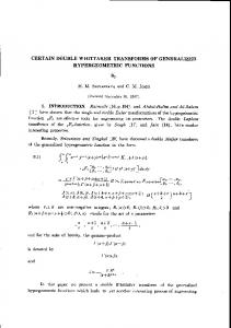
is univalued on C. Such a cycle is called a twisted cycle for the coefficient system defined by (12). A famous example of a twisted cycle is the Pochhammer contour (see figure 1) around the points 0 and 1. ✲

✻ ❄

t 0

1

t

✻ ❄

✲

Figure 1. The Pochhammer contour This has the advantage that we can remove the condition Re(c) > Re(a) > 0. Moreover, we obtain a linear map from the space of homology classes of twisted cycles in Yz = C\{0, 1, z1 }, to the space Vz of germs of local solutions at z: H1twist (Yz ) → Vz C→ ta−1 (1 − t)c−a−1 (1 − tz)−b dt . For generic parameters, phism.

C twist H1 (Yz )

(13)

is two dimensional and this map is an isomor-


5

Put X = C\{0, 1} and Y = C2 \{t = 0, t = 1, zt = 1}, and consider the projection π : Y → X, π(z, t) = z on the first coordinate. Y   π X

(z,t)  z

(14)

This projection is a fibration with fiber π −1 (z) = Yz . We define a vector bundle H1twist (Y /X) over X whose fiber at z is the twisted homology group H1twist (Yz ). An element Cz0 ∈ H1twist (Yz0 ) naturally defines a twisted cycle in every fiber H1twist (Yz ) if z is sufficiently close to z0 . Such local sections of H1twist (Y /X) are called flat, and this natural notion of flat local sections defines an integrable connection on the bundle H1twist (Y /X). This is the Gauss Manin connection of the fibration π (with respect to the twisting by the local coefficient system). The “flat continuation” of elements of H1twist (Yz0 ) defines a monodromy representation of Π1 (X, z0 ) in GL(H1twist (Yz0 )). In short, for generic parameters the isomorphism (13) interprets the monodromy action on the local solution space of the hypergeometric differential equation as the monodromy of the (twisted) Gauss-Manin connection of the fibration (14). When the parameters a, b and c are rational, we have a projection of the space of 1-cycles of the Riemann surface Zz of (12) to the space of twisted 1-cycles in the fiber Yz . Variation of z in the base space X should be thought of as a variation of moduli of the surface Z. The hypergeometric functions are now interpreted as period integrals, considered as functions of the moduli of Z. This point of view gives rise to modular interpretations of X (or certain local compactifications of it) via the Schwarz map S. This is the multivalued map on X defined by taking the projective ratio S(z) := (φ1 (z) : φ2 (z))

(15)

of two linearly independent solutions of the hypergeometric differential equation. Its branches are related to each other by the action of the projective monodromy group Γ+ . The S-image of the upper half plane X + ⊂ X is a circular triangle T called the Schwarz triangle. The vertices of T are the S-images of 0, 1, and ∞, and by (5), (7) and (8) its angles are (1 − c)π, (c − a − b)π, and (a − b)π

(16)

respectively. In order to avoid degeneracies we now assume that (a, b, c) is such that contiguous parameters give equivalent monodromy representations (this is true when a, b ≡ 0, c modulo Z). Applying contiguity relations repeatedly we can reduce T so that its angles are nonnegative, and that the sum of two angles is at most π. This ensures that the Schwarz map is a bijection from X + to T . By Schwarz’ reflection principle, Γ+ is realized explicitly as the normal subgroup of index two of holomorphic maps in the group Γ generated by the inversions in the edges of the Schwarz triangle T . By proper choice of the basis φ1 , φ2 in (15),

6

E. M. Opdam

T can be realized as a geodesic triangle in one of the three standard geometries. If the angle sum σ of T exceeds π, we can realize T as a geodesic triangle in D+ := P1 (C) (spherical case). When σ < π, we can realize T as a geodesic triangle in the upper half plane D− := H (hyperbolic case). Finally, when σ = π, we can realize T as a Euclidean triangle in D0 := C. We call T elementary when its angles are of the form πn with n ∈ {2, 3, . . .}. By elementary geometry in the natural geometric domain D ( = ±, 0) of T , the group Γ+ is a discrete subgroup of the group of isometries Aut(D ) if and only if T is finitely tesselated by copies of an elementary Schwarz triangle. When T is elementary, then its closure in its geometric domain D will be a fundamental domain for the action of Γ on D . When T is elementary, we can therefore find a holomorphic inverse J of S that extends to D by adding the points of finite branching order. The map J is automorphic for Γ+ and realizes an isomorphism ∼

˜ J : Γ+ \D −→ X

(17)

˜ is obtained from X by adding the points corresponding to the points of where X finite branching order. In the simplest case we consider a = b = 12 and c = 1. All angles of T are 0 now. In this case the Euler integral solutions of the hypergeometric differential equation are in fact the classical elliptic integrals. We find that Zz is a double cover of P1 (C) branched in 0, 1, ∞ and 1z , and this is an elliptic curve (with marked point of order two). The projective monodromy group is 1 0 modulo 2 . (18) Γ(2) = g ∈ PSL(2, Z) g ≡ 0 1 In this case, the inverse J is the lambda invariant that maps the quotient Γ(2)\H+ isomorphically to X = C\{0, 1}. It is an isomorphism between two natural models of the moduli space of elliptic curves with marked points of order two. We should think of the base space X = C\{0, 1} as the space of configurations of four points in P1 (C), i.e. the space of positions of four distinct points on the projective line, up to the simultaneous action of projective transformations on these points. In this way it is natural to generalize the above interpretation of the Euler integral to more general configuration spaces of geometric objects. This is a fruitful point of view for generalizing hypergeometric functions, which has led to applications in algebraic geometry. Configuration spaces are also natural to consider in mathematical physics, of course, and the hypergeometric functions in mathematical physics arise in this way also as functions of configurations. I shall return to these matters later. One variable generalizations like the functions p Fq and q-deformations like the basic hypergeometric series are certainly important, but we shall restrict ourselves to discussing multivariable generalizations in this overview.


7

2. Generalizations of Euler’s Hypergeometric Integral The first generalization of hypergeometric functions that comes to mind when we consider the Euler integral is the Lauricella FD function. Let X(n) denote the space of n ≥ 4 distinct, marked points x1 , . . . , xn in P1 (C), modulo the action of PGL(2, C). The space X(4) is nothing but the base space X = C\{0, 1} we considered in the previous section, since we can send the first three points to 0, 1 and ∞ by a uniquely determined fractional linear map, leaving the fourth point as a free variable in X.

Let µ be an n tuple of complex numbers with µi = 2. Let wµ denote the multivalued (1, 0)-form wµ =

n (t − xi )−µi dt

(19)

i=1

on Yx := P1 (C) − {x1 , . . . , xn}. For any twisted cycle C in Yx with respect to this form, we define the the following hypergeometric integral wµ . (20) IC (x) := C

These integrals are solutions of the Lauricella hypergeometric equations of “type D” when we fix xn−2 = 0, xn−1 = 1, and xn = ∞ and think of the IC (x) as functions of the remaining n − 3 variables. It is known that this is an n − 2 dimensional space V (µ) of multivalued functions on X(n). Choose a base point b ∈ X(n). The map C → IC (x) defines an isomorphism H1twist (Yb ) and the space V (µ)(U ) where x ∈ U and U is a suitable neighborhood of b. The analog of the Schwarz map in this context was studied by Picard (n = 5) [35], Terada [37], Deligne and Mostow [8, 9] and others. It was shown that when µi ∈ (0, 1), the space of twisted cycles H1twist (Yx ) carries an hermitian intersection form M of signature (1, n − 3), invariant for monodromy. Hence, for a suitable choice of basis Ci of H1twist (Yb ), the image of the Picard-Schwarz map P S : X(n) → Pn−3 (C) x → (IC1 (x) : · · · : ICn−2 (x))

(21) (22)

is inside the set B = {z = (z1 : · · · : zn−2 )|M (z, z) > 0}. The space B is isomorphic to the unit ball in Cn−3 . The main theorem of [8] asserts that the projective monodromy group Γ(µ) ⊂ P U (1, n − 3) is discrete if there exist mi,j ∈ N ∪ ∞ such that 1 − µi − µj = m1i,j or 2 −1 extends mi,j when µi = µj . Moreover, the image of P S is dense in B, and P S holomorphically to B and gives an isomorphism ˜ P S −1 : Γ(µ)\B → Σ\X(n)

(23)

˜ where Σ is the group of permutations of points xi with equal weights µi , and X(n) is some quasi projective local compactification of X(n).

8

E. M. Opdam

This is a delightful generalization of the theory of the Schwarz map. At the same time it is clear that it is not the end of the story! Other generalizations of the hypergeometric function can be obtained easily by considering hypergeometric integrals associated with configuration spaces of hyperplanes in Pn (C). For example, Yoshida obtained the modular interpretation of the configuration space X(3, 6) of 6 lines in P2 (C) in his book [39]. Other work in this direction was done by Couwenberg [7], working with the root system type hypergeometric functions that will be discussed in section 3. Many open problems remain in this direction. 2.1. The Gelfand-Kapranov-Zelevinskii-hypergeometric function This hypergeometric function (sometimes called A-hypergeometric function) was introduced in [15]. It is in fact a very general class of hypergeometric functions that resembles the case of Lauricella functions. The classical generalizations of the Gauss hypergeometric function like p Fq , the Lauricella type functions, and Horn’s hypergeometric functions all occur as special cases of the GKZ-systems. The GKZ-hypergeometric functions are defined by means of a deceptively simple system of differential equations. Let A ⊂ Zn be a finite generating subset of Zn . Assume that A lies inside a rational hyperplane. In other words, there exists a linear function h : Zn → Z such that h(A) = 1. Let L ⊂ ZA denote the lattice of relations in A, thus aω ω = 0} . (24) L := {(aω ) ∈ ZA | ω∈A

For a ∈ L, define a constant coefficient partial differential operator a on CA by ∂ aω ∂ aω − . (25) a := ∂xω ∂xω aω >0 aω