Multivariable Multirate System Description and Design - Science Direct

Copyright © IFAC Control of Industrial Systems, Belfon. France, 1997

MULTIVARIABLE MULTIRATE SYSTEM DESCRIPTION AND DESIGN Ryszard Gessing Politechnika Slqska Instytut A utomatyki, ul. Akademicka 16, 44-101 Gliwice, Poland, fax: +4832371165, email: gessing @ ia. gliwice.edu.pl

Abstract: It is shown that for a multirate (MR) system the discrete-time (DT) transfer function (TF) description exists only in a rather seldom case when the sampling period of input is integer multiple of that of the output. It is also noticed that in other cases, especially in the case of multivariable (MV) systems the whole system cannot be described by using TF method. For the MV MR system a continuous-time (CT) model is proposed which makes it possible to obtain the controllers by using some appropriate CT method of design and the DT Tustin approximation. Finally , the example of two variable, tworate system illustrating the proposed methods is considered. Resume: On peut constater que pour le systeme avec des periodes diverses d'echantillonage de 1'entree et de la sortie du systeme, une description de transmittance discret n'existe que dans le cas, quand la periode d'echantillonage de l'entree est une propre multiple de la periode d'echantillonage de la sortie. Dans le cas du systeme multivariable avec des periodes diverses d'echantillonage, le systeme integral ne peut pas etre decrit par une transmittance discrete. Dans ce cas, on propose un modele continu de l'objet qui facilite la synthese des regulateurs a la base du methode de temps continu et d'approximation de Tustin. A la fin, on a applique la methode proposee pour un exemple de ce systeme avec deux etats variables et deux periodes diverses d 'echantillonage. Keywords: Multivariable systems; multirate systems; systems design.

1.

I~TRODUCTION

(CL) systems. In the present paper

Discrete-time (DT), multirate (MR) systems having samplers with various sampling periods have rather a long history. In second half of fifties Kranc (1957) proposed his operator for analysing these systems. The systems have been described by Kuzin (1962) in his excellent book. A recapitulation in which the state of art related to these systems is given in the survey paper of Araki (1993).

• the cases when the open-loop (OL) TF exists and not exists are discussed: • in the case of multivariable (MV) Y1R systems when the TF description does not exist, the proposition is given based on applying the continuous-time (CT) models and adapting the method of design described by Gessing (1995a).

It should be stressed that the MR systems for the case when the sample periods are not integer multiples of each other usually can't be described by the DT transfer functions (TF)'s since these systems are nonstationary. In connection with this some difficulties arise in describing the closed-loop

2. MULTIVARIABLE

~fULTIRATE

SYSTEM

Consider the MV MR system shown in Fig.l. composed of CT multi-input and multi-output plant

705

described by the matrix TF

Let us introduce the following notation ex:

yh(Z)

(1)

= 2 h[y(nh)] = L

y(nh)z-n

(2)

n=O

and m independent feedback channels with samplers having different sampling periods hi , zero order holds ZOH i and DT controllers described by DT TF's ~(z), i = L 2, ... , m. The different sampling periods applied in different channels can be justified by different velocities of particular channels, as well as by limitations resulting from applied measurement devices.

i.e. the symbol 2h denotes the 2-transform for the sampling period h. In the Case 1 for any DT series [u(nlYh)] and [y(nh)], n 0,1,2, ... it is

=

00

Yi(nh)

The considered system is linear, but the whole system can not be described by using TF method. Really, the TF description of the whole system from Fig.1 would be possible if would exist the TF for the system shown in Fig.2 in the case of different sampling periods hi, h j . Thus there arises the question: whether and when there exists the TF for the system from Fig.2 ? It should be stressed that in the available literature there is no exact answer to this question, though the problem of possible nonexistence of a TF is noticed e.g. in (Program CC, 1991).

= 2:)u(lNh) -

u((l- 1)Nh)] .

1=0

·Yij(nh-INh)

(3)

where

(4) and .c -1 denotes the symbol of inverse Laplace transform. From applying 2-transform to both sides of (3) it results

00

yh(Z) = L[u(lNh) - u((l- 1)Nh)]. 1=0

·2h[§ij(nh)]z-IN =

= (1- z-N)UNh(z)2h[§ij(nh)] ~l

Ri (ll

-

J

(5)

or

'I

h :\'"

R..(1I

- ... f

(6)

m

where

Fig. 1 DT multivariable multirate system.

00

UNh(ZN) = L

Fig. 2 DT system with hi

#

u(lN h)(zN)-1

(7)

1=0

hj .

3. PROBLEM OF TRANSFER EXISTENCE

FCNCTIO~

Thus, for the Case 1 there exists the TF (8) which relates the DT output yh(z) to any DT input UNh(zN).

Consider the three cases: Case 1 : hi = h. hj = ."ih, .J\'-an integer: Case 2 : hi ,'vI h. hj = h, M -an integer: Case 3: hi = ,'vIh, hj = Nh, M,N-somemutual first integers.

From the other hand, in the Case 2 it can be noticed that then,does not exist the TF which relates the input and output signals. The cause is that the system is then nonstationary. Really, iffor any input uj(nh) the system output is Yi(nMh), n = 0,1,2, ... , then for the shifted by h in time input Uj (nh - h) the output Yi is not shifted by

=

Here h denotes some basic time interval (greatest common devisor of hi, h j ).

706

:..Jj

Also in the Case 3 the TF of the system shown in Fig.2 does not exist since the system is nonstationary: too.

w; :..;;'

From above considerations it results that the whole MV MR system shown in Fig.1 can not be described by using the TF method. This creates an essential difficulty in designing this kind of systems.

Since the models with derivative (Gessing. 1995a) are simpler they will be preferred for using in the case of CT plants without delay. In the case of CT plants with delay the use of the model with delay is justified since then no increase of design complexity is obtained.

4. MULTIVARIABLE MULTIRATE SYSTEM DESIG:"

5. A METHOD OF DESIGN OF CT MV SYSTEMS

Consider the system shown in Fig.1. Assume that in the control structure shown there, the input Uj of the plant is appropriately suited to the output Yj, i = 1,2, ... , m , so that both appear in the i-th control channel. Since the whole system can not be described by means of a DT TF it is reasonable to use an appropriate CT model of the plant with ZOH, described for the SISO case in (Gessing, 1995a). Using this model the following design algorithm of DT MV systems can be proposed.

Now, consider the CT MV system shown in Fig.1 in which the samplers and ZOH's disappear and the DT controllers Rj (z) are replaced with the CT ones Rj(s). Here, the approach will be proposed which makes it possible to apply a one variable design method, repeatedly. The approach is based on a repetitive procedure in which the CT controller R j (s) in the j-th loop is designed for the replacement SISO plant resulting from accounting the remaining loops closed (those which already have designed controllers).

4.1. Design algorithm

Thus, first the controller R l (s) is designed for the plant G l l (s); the remaining loops are open since they have no designed controllers, yet. Second controller R2( s) is designed for the 2-nd replacement SISO plant resulting from accounting the first loop closed and the remaining open: tird - for the 3-rd replacement SISO plant with accounting two first loops closed and the remaining open; finally, the m-th controller R m (s )-for the m-th replacement SISO plant resulting from accounting all the remaining loops closed.

1) For given TF's Gij(s) and assumed sampling periods h j create the modified TF's - with the derivative G1j (s) = (1-sh j /2)Gjj (5) or with delay

Gij(s)

= exp(-shj /2)G jj (s),

i,j

= 1,2, ... ,m;

2) Using one from the known methods of design of CT MV systems choose the CT controllers Rj (5), j = 1,2, ... , m, for the eT plant described by modified with the derivative (or with the delay) TF's;

3) Check if the sampling periods h j are sufficiently small, i.e. if the sampling frequency Wj = 21r/h j is approximately ten times greater than the appropriately calculated bandwidth frequency of the j-th loop; if not - decrease the sampling period h j and repeat the steps 1) and 2);

Then, we repeat our design procedure starting from the first loop and designing the controller Rj(s) in the j-th loop, j = 1. 2, ... , m for the j-th replacement SISO plant resulting from accounting all the remaining loops closed with the controllers designed in the latter steps. If needed, we repeat the design procedure until the further steps give no improvement of the control.

w;

4) The DT controllers Rj(z) result from using the Tustin approximation of the CT controllers Rj (s), j 1,2 .... , m, i.e.

=

-1)

( nz+1 ~z

w;,

~ first the bandwidth frequencies :..;;' can be determined for the CT system with the controllers R j (s) designed for the multi variable plant G(s). Next, we can assume that ~ and determine hj'

h since the minimal shift in time for the output is Mh.

It should be stressed that the proposed design procedure is usually fastly convergent. This is the result of the fact that the change of the controller Rj (s) in the j-th loop influences mainly the characteristics of the j-th open loop. The characteristics of the remaining open loops are significantly less influenced, since for them the loop with R j (s) is closed and - less sensitive to parameters change .

(9)

w;

The bandwidth frequency for each j- th loop is calculated with accounting the remaining m - 1 loops of the system closed.

.".'ote. In order to choose the proper sampling periods h j assuring the fulfilment of the condition

707

-----

l.'--~--~-

6. EXAMPLE :2

~

A'

I

Consider the DT two variable tworate system shown in Fig.l in which the plant matrix TF is determined by

I

/

o.e,

//

106r

//

~;

/,

o.,~ I

10 S(Si 1 )'

G(s) =

~

,1

(5+2)j5+3) ]

[ 5(5+1) ,

;/

/!

Ij

02:

o:..v

( 10)

(5+2)(5+3)

I

_

er model ....ith derivative:

- -

DT system with hI =0.18 and h2=0.24.

· 0 . 2 - - - - - - - - - - - - -S - - UIU

The DT TF's RI(z) and R2 (z) are to be designed which determine the algorithms for the DT controllers of both loops.

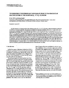
Fig. 4 Step responses of the second output.

=

After some preliminary trials it is assumed hI 0.18 and h 2 = 0.24 . The model with derivative takes the form Gd (

-0.95+10 5(5+1)'

) _

s -

[

-0.455+5 5(5+1) ,

-0.845+7 ] (5+2)(5+3) -0.845+7 (5+2)(5+3)

R (5) I

= 0.4 0.85 +

1 0.15 + 1 '

R Z(5)

= -2.6 5

(11)

The bandwidth frequencies of both the loops with appropriate replacement 5ISO plants are wi = 3.57 and Wz = 1.27. Since WI = 21r10.18 = 34.9 and Wz = 21r10.24 = 26.1 then wdwi = 9.78 and wz/wz == 20.55. The DT controllers are determined by the TF's resulting from the Tustin approximation of (13)

First, the CT controllers Rj (5) j = 1, 2 are designed using the method described in the previous section and illustrated in (Gessing, 1995b). In the first step the controller R~ (5) is designed for the plant Gf I (5). In the second step the controller R~( 5) is designed for the replacement 5150 plant of the second loop described by the TF

R (z) = 1.873684(z - 0.7977528) I z - 0.05263158 ' R 2(5) = 0.312(z + 1) z- 1

In the third step the controller R~ (5) is designed for the replacement 5150 plant of the first loop described by

R;

7. FINAL CONCLUSIONS

lZ--~-----~-------

::~ i/

-

For MR 5ISO systems the DT TF description exists only in some rather seldom cases when the sampling period of input is integer multiple of that of the output. In other cases the MR 5ISO systems can not be described by means of TF. The MY MR systems can not be described by the TF method, which creates some essential difficulties in their description and design.

er model with derivarive~ DT system "'ith hl=0.18 and h2=0.24.

; •.1

o:t .'

f-!

'el,-I

(IS)

In Fig. 3, 4 the step responses of both the loops and in Fig. 5, 6 the interaction responses of the CT system described by (12) and (14) are compared with those of DT system described by (10) and (15). 5ince, for the DT system the TF description does not exist the appropriate transients were determined by means of SIMULINK program, ver .1.3c. It is seen that both transients of the CT model with derivative and of the DT system are mutually very close.

(5) for the reIn the forth step the controller placement 5150 plant G;' (determined by (11) with R~ replaced by R~ ) -is designed which however gives no essential improvement of the control. Finally, the CT controllers are described by the TF's:

.. ,

(14)

--'

o

The proposed method of design of MY MR systems. based on the approximate plant TF's j (5)

G1

Fig. 3 5tep responses of the first output.

708

or G'fj (s) and the Tustin approximation of the designed CT controllers makes it possible to design the MV MR systems. practically without knowledge concerning the description of DT systems.

ACKNOWLEDGEMENT The paper was partially supported by Science Research Committee grant Ko 8 TllA 031 10. REFERENCES

L,,--_--

0.5

--

-

CT model with

--

Araki M. (1993). Recent Developments in Digital Control Theory. Preprints of the 12-th IFAC World Congress, Sydney, July 1993. pp. 251-260.

derivative~

Kranc, G.M. (195i). Compensation of an Error Sampled System by a Multi-rate Controller. Trans. A lEE, 76, Pt.IIl, pp.149-159. ·O.2L--------------------' 5

J

Fig. 5 Time responses of Y2 for

Wl

Kuzin, L.T. (1962). Calculation and Design of Discreie- Time Systems. Moskow (in Russian).

bm~

= l(t).

Program CC (1991). Tutorial and User's Guide. System Technology Inc. California.

0.8

::. 06

-

CT model with derivati"";

- -

DT system with hl~O.18 and h2~O.24.

Gessing, R. (1995a). Comments on "A Modification and the Tustin Approximation" with a Concluding Proposition. IEEE Trans. Autom. Contr., 40, no. 5, pp. 942- 944.

Ii

Gessing, R. (1995b). Discrete-Time Multivariable System Design by Means of Continuous-Time Methods. Preprints of the IFACjIFIPjIMACS Symposium: Large Scale Systems Theory and Applications, London, pp.135-139.

/,

02r

I

/

00 I

·D.2L-------------------' 5

C

Fig. 6 Time responses of Yl for

W2

Illll.

= l(t).

SIMULINK (1993). Dynamic System Simulation Software User's Guide. The Math. Works Inc.

709