Multivariate Extended Skew-t Distributions and Related Families
Reinaldo B. Arellano-Valle1 and Marc G. Genton2
October 19, 2009
Summary A class of multivariate extended skew-t (EST ) distributions is introduced and studied in detail, along with closely related families such as the subclass of extended skew-normal distributions. Besides mathematical tractability and modeling flexibility in terms of both skewness and heavier tails than the normal distribution, the most relevant properties of the EST distribution include closure under conditioning and ability to model lighter tails as well. The first part of the present paper examines probabilistic properties of the EST distribution, such as various stochastic representations, marginal and conditional distributions, linear transformations, moments and in particular Mardia’s measures of multivariate skewness and kurtosis. The second part of the paper studies statistical properties of the EST distribution, such as likelihood inference, behavior of the profile log-likelihood, the score vector and the Fisher information matrix. Especially, unlike the extended skew-normal distribution, the Fisher information matrix of the univariate EST distribution is shown to be non-singular when the skewness is set to zero. Finally, a numerical application of the conditional EST distribution is presented in the context of confidential data perturbation.
Keywords: Confidential data perturbation; Elliptically contoured distributions; Fisher information; Kurtosis; Non-normal; Skewness. Short title: Multivariate Extended Skew-t Distributions 1
Departamento de Estad´ıstica, Facultad de Matem´atica, Pontificia Universidad Cat´olica de Chile, Santiago 22, Chile. E-mail:
[email protected] This research was partially supported by grant FONDECYT 1085241-Chile. 2 Department of Statistics, Texas A&M University, College Station, TX 77843-3143, USA. E-mail:
[email protected] This research was partially supported by NSF grants DMS-0504896, CMG ATM-0620624, and by Award No. KUS-C1-016-04, made by King Abdullah University of Science and Technology (KAUST).
1
Introduction
The quest for flexible parametric families of multivariate distributions has received sustained attention in recent years as witnessed by the book edited by Genton (2004), the review of Azzalini (2005), and references therein. Although the families under consideration can be casted in a unified framework of skewed distributions arising from certain selection mechanisms (ArellanoValle et al., 2006), the multivariate skew-t distribution has emerged as a tractable and robust model with parameters to regulate skewness and kurtosis in the data. Azzalini and Genton (2008) have advocated its use by means of various theoretical arguments and illustrative examples. Nevertheless, the skew-t distribution has some shortcomings and we propose to address them in this article. First, the skew-t distribution is not closed under conditioning. This is an important issue for methods that require the study of the conditional distribution of a skew-t model fitted to the data. For instance, various data perturbation methods require to simulate from the conditional distribution of confidential variables given non-confidential ones, see Muralidhar and Sarathy (2003) for a recent review and references therein. Similarly, certain imputation methods for censored data necessitate to replace censored observations by values simulated from a conditional distribution, see for example Park et al. (2007) for the case of censored time series. Second, although the skew-t distribution has the ability to model distributional tails that are heavier than the normal, it cannot represent lighter tails. Those issues can be circumvented by the following definition of an extended version of the skew-t distribution. Definition 1 (Extended skew-t) A continuous p-dimensional random vector Y has a multivariate extended skew-t (EST) distribution, denoted by Y ∼ ESTp (ξ, Ω, λ, ν, τ ), if its density function at y ∈ Rp is ( ) µ ¶1/2 ¡ T ¢ ν+p 1 √ t (y; ξ, Ω, ν) T1 λ z + τ ;ν + p , (1) ¯ ν) p ν + Q(z) T1 (τ / 1 + λT Ωλ; ¯ −1 z, λ ∈ Rp is the shape parameter, τ ∈ R is the extension where z = ω −1 (y − ξ), Q(z) = z T Ω parameter, µ ¶−(ν+p)/2 Q(z) Γ((ν + p)/2) 1+ tp (y; ξ, Ω, ν) = |Ω|1/2 (νπ)p/2 Γ(ν/2) ν denotes the density function of the usual p-dimensional Student’s t distribution with location ξ ∈ Rp , positive definite p × p dispersion matrix Ω, with p × p scale and correlation matrices ω = ¯ = ω −1 Ωω −1 , respectively, and degrees of freedom ν > 0, and T1 (y; ν) denotes the diag(Ω)1/2 and Ω univariate standard Student’s t cumulative distribution function with degrees of freedom ν > 0. The EST distribution provides a very flexible class of statistical models. In fact, for λ = τ = 0, we retrieve the multivariate symmetric Student’s t distribution, tp (ξ, Ω, ν), which reduces to the multivariate normal Np (ξ, Ω) and Cauchy Cp (ξ, Ω) distributions by letting ν → ∞ and ν = 1, respectively. The same occurs when τ → +∞, while for τ → −∞ the density degenerates to 1
zero. For τ = 0, we have the multivariate skew-t distribution STp (ξ, Ω, ν, λ) in the form adopted by Azzalini and Capitanio (2003). The multivariate skew-normal SNp (ξ, Ω, λ) distribution of Azzalini and Dalla Valle (1996) and the skew-Cauchy SCp (ξ, Ω, λ) distribution of Arnold and Beaver (2000a) arise when we further let ν → ∞ and ν = 1, respectively. For λ = 0, the following new family of symmetric densities is obtained: ( µ ) ¶1/2 1 ν+p tp (y; ξ, Ω, ν) T1 τ ;ν + p , (2) T1 (τ ; ν) ν + Q(z) d
which corresponds to the density of ξ + CZ, where Z = (X|X0 + τ > 0) with (X T , X0 )T ∼ tp+1 (0, Ip+1 , ν), a Student’s t distribution, and C = Ω1/2 , i.e., a square root of Ω. Finally, for ν → ∞ we obtain the extended skew-normal ESNp (ξ, Ω, λ, τ ) distribution with density √
1
¯ Φ1 (τ / 1 + λT Ωλ)
¡ ¢ φp (y; ξ, Ω) Φ1 λT z + τ ,
(3)
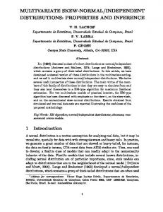
which arose with a slightly different parameterization in Azzalini and Capitanio (1999) and Arnold and Beaver (2000b). The ESN distribution has been studied in more detail by Capitanio et al. (2003), although without noticing that lighter tails than the normal distribution could be obtained for certain values of τ . We examine this interesting property in this paper. Finally, we note that Azzalini and Capitanio (2003, Sec. 4.2.4) also briefly sketched the definition of an extended skew-t distribution, although with a normalization based on the normal cumulative distribution function Φ1 instead of T1 . Such an extension of the skew-t distribution does not seem to be as natural as (1). In order to illustrate the shape of the extended skew-t distribution, we start by setting p = 1. In this case, a random variable Y ∼ EST1 (ξ, ω 2 , λ, ν, τ ) has a density of the form ( ) µ ¶1/2 ν+1 1 2 √ t1 (y; ξ, ω , ν) T1 (λz + τ ) ;ν + 1 , (4) ν + z2 T1 (τ / 1 + λ2 ; ν) where z = (y − ξ)/ω. Figure 1 depicts the density (4) for ξ = 0, ω = 1, λ = 2, ν = 3, and various values of τ . The solid thick curve corresponds to τ = 0, that is, the classical ST density. For τ = 1, 3, 5 (solid curves), the densities become more symmetric and approach the t1 (y; ξ, ω 2 , ν) density. For τ = −1, −3, −5 (dashed curves), the densities become more skewed. The moments of the EST distribution will be developed in this paper. For illustration, we p present in Figure 2 the mean µ, variance σ 2 , and coefficients of skewness β1,1 and kurtosis β2,1 of the univariate standard extended skew-normal distribution, that is ESN1 (0, 1, λ, τ ), as a function of τ for λ = 1, 2, 3, 4, 5. The thick curve is for λ = 1. It can be observed that for certain values of τ > 0, the kurtosis β2,1 < 0, indicating lighter tails than the normal distribution. Although the extended skew-t distribution of Definition 1 is appealing for practical applications, there are two natural generalizations that are of interest from a theoretical point of view. First, a continuous p-dimensional random vector Y has a multivariate unified skew-t (SU T ) 2
0.5
τ=0 τ=−1
τ=−3
0.3
τ=3
τ=−5
τ=5
0.0
0.1
0.2
density
0.4
τ=1
−2
0
2
4
6
y Figure 1: Densities of the EST1 (0, 1, 2, 3, τ ) for τ = 0 (thick solid curve), τ = 1, 3, 5 (solid curves) and τ = −1, −3, −5 (dashed curves). distribution, denoted by Y ∼ SU Tp,q (ξ, Ω, Λ, ν, τ, Γ), if its density function at y ∈ Rp is ) ( ¶1/2 µ 1 ν+p ; Γ, ν + p , ¯ T , ν) tp (y; ξ, Ω, ν) Tq (Λz + τ ) ν + Q(z) Tq (τ ; Γ + ΛΩΛ
(5)
where now Λ is a q × p real matrix controlling shape, τ ∈ Rq is the extension parameter, Γ is a q × q positive definite correlation matrix, and Tr (y; Σ, υ) denotes the r-dimensional centered Student’s t cumulative distribution function with r × r positive definite dispersion matrix Σ and √ degrees of freedom υ > 0. For q = 1, we have that Γ = 1, Λ = λT and Tq (x; a, ν) = T1 (x/ a; ν), hence (5) reduces to (1), that is, SU Tp,1 = ESTp . When ν → ∞ it reduces to the following unified skew-normal (SU N ) density 1 ¯ T ) φp (y; ξ, Ω) Φq (Λz + τ ; Γ) , Φq (τ ; Γ + ΛΩΛ which is denoted by SU Np,q (ξ, Ω, Λ, τ, Γ) and was studied in Arellano-Valle and Azzalini (2006) with a different but equivalent parameterization. Although numerical algorithms exist to evaluate 3
1.0 0.8
10
0.6
8
σ2
6
0.4
µ
0.2
4
0.0
2 0
−10
−20
−10
0
10
20
0
10
20
τ
−20
−10
−20
−10
0
10
20
0
10
20
τ
0.0
0.0
0.2
0.5
0.4
β21
β11
0.6
1.0
0.8
1.5
1.0
−20
τ
τ
p Figure 2: Mean µ, variance σ 2 , and coefficients of skewness β1,1 and kurtosis β2,1 of the univariate standard extended skew-normal distribution, that is ESN1 (0, 1, λ, τ ), as a function of τ for λ = 1, 2, 3, 4, 5. The thick curve is for λ = 1. the multivariate cumulative distribution functions Φq and Tq for q > 1, see Genz (1992) and Genz and Bretz (2002), this aspect is less appealing from a practical point of view than using q = 1. The SU T and the SU N are only two important subclass of a more general family originating from elliptically contoured (EC) distributions (see, e.g., Fang et al., 1990) that we describe next. A continuous p-dimensional random vector Y has a multivariate unified skew-elliptical (SU E) distribution, denoted by Y ∼ SU Ep,q (ξ, Ω, Λ, h(p+q) , τ, Γ), if its density function at y ∈ Rp is ³ ´ 1 (q) (p) f (y; ξ, Ω, h ) F Λz + τ ; Γ, h q Q(z) , ¯ T , h(q) ) p Fq (τ ; Γ + ΛΩΛ where fp (y; ξ, Ω, h(p) ) = |Ω|−1/2 h(p) (Q(z)) denotes the density function of an elliptically contoured distribution with location ξ ∈ Rp , positive definite p × p dispersion matrix Ω, and density generator h(p) , Fr (y; Σ, h(r) ) denotes the r-dimensional centered elliptical cumulative distribution (q) function with r × r dispersion matrix Σ and density generator h(q) , and hQ(z) (u) = h(p+q) (u + 4
Q(z))/h(p) (Q(z)). The SU E distribution was also considered in Arellano-Valle and Azzalini (2006) with a different but equivalent parameterization, see also Arellano-Valle et al. (2006) and Arellano-Valle and Genton (2005). However, these authors did not study systematically the main properties of the SU E distributions, for instance such as marginal and conditional distributions, and moments. The SU E distribution reduces to the SU T when h(p) is the pdimensional Student’s t density generator function with ν degrees of freedom, that is, h(p) (u) = c(ν, p) {1 + (u/ν)}−(ν+p)/2 ,
where c(a, b) =
Γ((a + b)/2) . Γ(a/2)(πa)b/2
(6)
Moreover, when q = 1 the SU E distributions will be called extended skew-elliptical (ESE) distributions by analogy with Definition 1. They reduce directly to the EST distributions when adopting the Student’s t density generator function (6). The paper is now organized as follows. We present the probabilistic properties of the EST distribution in Section 2. Their proofs are given in the Appendix. Those theoretical properties include various stochastic representations, marginal and conditional distributions, linear transformations, moments and in particular Mardia’s measures of multivariate skewness and kurtosis. In Section 3, we study statistical properties of the EST distribution, such as likelihood inference, behavior of the profile log-likelihood, the score vector and the Fisher information matrix. Especially, the Fisher information matrix of the univariate EST distribution (hence also the ST ) is shown to be non-singular when the skewness is set to zero, unlike the case of the ESN distribution (hence also the SN ). Finally, we present a numerical application of the conditional EST distribution in the context of confidential data perturbation.
2 2.1
Probabilistic Properties Stochastic Representations
We present three stochastic representations of the EST distribution. They are useful for the generation of random numbers and for deriving moments and other formal properties. Proposition 1 (Selection representation of EST) Let Y = ξ + ωZ, where d
Z = (X|X0 < λT X + τ ) and
Ã
X X0
!
ÃÃ ! Ã ! ! ¯ 0 Ω 0 , ,ν . ∼ tp+1 0 0 1
(7)
(8)
Then Y ∼ ESTp (ξ, Ω, λ, ν, τ ). The stochastic representation (7) is a natural extension of a stochastic representation considered by Azzalini (1985) to introduce the univariate skew-normal distribution. There are however 5
two other equivalent and convenient stochastic representations for Z, which yield the well-known δ-parameterization of the shape parameter. These stochastic representations are given next. ˜ 0 = (1 + λT Ωλ) ¯ −1/2 (λT X − X0 ) and τ¯ = (1 + λT Ωλ) ¯ −1/2 τ. Then First, let X d
˜ 0 + τ¯ > 0), Z = (X|X where
Ã
X ˜0 X
!
ÃÃ ∼ tp+1
0 0
! Ã ,
¯ δ Ω δT 1
!
(9)
! ,ν
,
and δ = √
¯ Ωλ ¯ 1 + λT Ωλ
.
(10)
The representation (9), sometimes called a conditioning method, was used by Azzalini and Dalla Valle (1996) to introduce the multivariate skew-normal distribution and also by Branco and Dey (2001) to extend this model to skew-elliptical distributions. This stochastic representation yields the δ-parameterization on (−1, 1)p of the shape parameter. Therefore, we need to make a reparameterization from δ to λ in order to express the model in term of the λ-parameterization in Rp . Another advantage of this stochastic representation is that it allows to obtain the distribution of functions ψ(Z), for example such as linear functions, in a simple way, because d ˜ 0 + τ¯ > 0). ψ(Z) = (ψ(X)|X ˜ = X − δX ˜ 0 . Then Second, let X d ˜ + δX ˜ 0 )|X ˜ 0 + τ¯ > 0], Z = [(X
where
Ã
˜ X ˜0 X
!
ÃÃ ∼ tp+1
0 0
! Ã ,
¯ − δδ T 0 Ω 0 1
(11) !
! ,ν
.
d ˜ d ˜ (−¯τ ,∞) , where X ˜ (−¯τ ,∞) = ˜ 0 |X ˜ 0 + τ¯ > 0), when The representation (11) reduces to Z = X + δX (X ˜ and X ˜ 0 are independent, which holds for the normal distribution (i.e., ν → ∞) only. In X that case, it is sometimes called a convolution method and is useful to compute moments, to perform simulations, and also to implement both the EM algorithm and MCMC procedures. For additional comments about the different but equivalent representations (7), (9) and (11), see Arellano-Valle and Azzalini (2006) and Arellano-Valle et al. (2006). We give in Proposition 2 below a novel and very convenient convolution type of representation for the EST random vector Z, which is based on (11).
Proposition 2 (Convolution type stochastic representation of EST) Let Z be a p × 1 random vector defined by s 2 ν + T(−¯ τ ,∞) Z= X1 + δT(−¯τ ,∞) , (12) ν+1 d ¯ − δδ T , ν + 1) and is independent of T(−¯τ ,∞) = where X1 ∼ tp (0, Ω (X0 |X0 + τ¯ > 0), with X0 ∼ ¯ t(0, 1, ν). Then Z ∼ ESTp (0, Ω, ν, λ, τ¯).
6
The cumulative distribution function of the EST distribution can also easily be computed from (7) or (9). Indeed, if Y ∼ ESTp (ξ, Ω, λ, ν, τ ) then ÃÃ ! Ã ! ! ¯ −δ z Ω 1 P (Y ≤ y) = Tp+1 ; ,ν + 1 , T1 (¯ τ ; ν) τ¯ −δ T 1 where z = ω −1 (y − ξ) and τ¯ and δ are defined above. ¯ λ, τ ) Let Z = V −1/2 Z0 , where the random scale factor V is defined on (0, ∞), Z0 ∼ ESNp (0, Ω, ¯ λ, τ ), and they are independent. By conditioning on V = v, we have (Z|V = v) ∼ ESNp (0, v −1 Ω, that is, a conditional ESN density given by fZ|V =v (z) =
1 ¯ 1 (v 1/2 λT z + τ ). φp (z; v −1 Ω)Φ Φ1 (¯ τ)
(13)
Thus, if for example we assume in (13) that V ∼ Gamma(ν/2, ν/2), then we can conclude that the ST distribution (but not the EST distribution) can be expressed as a scale mixture of the skew-normal distribution. In other words, from (13) and E{fZ|V (z)} = fZ (z) we have for τ = 0 that: ) ( ¶1/2 µ © p/2 ª ν + p ¯ 1 (V 1/2 λT z) = tp (z; Ω, ¯ ν)T1 λT z ;ν + p . E V φp (V 1/2 z; Ω)Φ ν + Q(z) Hence, if Y ∼ ESTp (ξ, Ω, λ, ν, τ ), then only for τ = 0 we obtain the following well-known stochastic representation of the ST distribution as a scale mixture of the SN distribution: d
˜ Y = ξ + ωV −1/2 Z, ¯ λ). where V ∼ Gamma(ν/2, ν/2) and is independent of Z˜ ∼ SNp (0, Ω,
2.2
Distribution Theory
We start by describing the marginal distribution of the EST . Proposition 3 (Marginal distribution of EST) Let Y ∼ ESTp (ξ, Ω, λ, ν, τ ). Consider the partition Y T = (Y1T , Y2T ) with dim(Y1 ) = p1 , dim(Y2 ) = p2 , p1 + p2 = p, and the corresponding partition of the parameters (ξ, Ω, λ). Then Yi ∼ ESTpi (ξi , Ωii , λi(j) , ν, τi(j) ) for i = 1, 2, where λi(j)
¯ ij λj ¯ −1 Ω λi + Ω ii , =q ˜ jj·i λj 1 + λTj Ω
τ τi(j) = q , ˜ jj·i λj Ω 1 + λT j
¯ ij , ˜ jj·i = Ω ¯ jj − Ω ¯ ji Ω ¯ −1 Ω Ω ii
for i = 1, 2 and j = 2, 1. Note that λ2 = 0 with λ1 6= 0 does not implies symmetry in the marginal distribution of Y2 . ¯ ¯ −1 In fact, a necessary and sufficient condition to obtain λ2(1) = 0 is that λ2 = −Ω 11 Ω12 λ1 . Next, we present the conditional distribution of the EST and emphasize that the resulting distribution remains in the original family. 7
Proposition 4 (Conditional distribution of EST) Let Y ∼ ESTp (ξ, Ω, λ, ν, τ ). Consider the partition Y T = (Y1T , Y2T ) with dim(Y1 ) = p1 , dim(Y2 ) = p2 , p1 +p2 = p, and the corresponding partition of the parameters. Then ∗ (Y2 |Y1 = y1 ) ∼ ESTp2 (ξ2·1 , αQ1 Ω22·1 , λ2·1 , ν2·1 , τ2·1 ), −1 −1 T ¯ −1 where ξ2·1 = ξ2 +Ω21 Ω−1 11 (y1 −ξ1 ), Q1 (z1 ) = z1 Ω11 z1 , z1 = ω1 (y1 −ξ1 ), Ω22·1 = Ω22 −Ω21 Ω11 Ω12 , ¯ ¯ −1 λ2·1 = ω2·1 ω2−1 λ2 , ω2 = diag(Ω22 )1/2 , ω2·1 = diag(Ω22·1 )1/2 , ν2·1 = ν + p1 , τ2·1 = (λT 2 Ω21 Ω11 + −1/2 ∗ λT 1 )z2 + τ , τ2·1 = αQ1 τ2·1 and αQ1 = (ν + Q1 (z1 ))/(ν + p1 ).
Unlike the marginal distribution of Y2 , we note for the conditional distribution of Y2 given Y1 = y1 that λ2 = 0 implies symmetry. Another interesting consequence of the result in Proposition 4 is that even if one starts with an ST distribution, that is an EST with τ = 0, then ∗ the resulting conditional distribution has an extension parameter τ2·1 6= 0, unless the condition −1 ¯ 11 Ω ¯ 12 λ2 holds or z1 = 0. In order to illustrate this effect, consider the bivariate random λ1 = −Ω vector Y ∼ EST2 (0, I2 , λ, ν, 0) ≡ ST2 (0, I2 , λ, ν). Then the conditional distribution is s à ! ν+1 ν + y12 , λ2 , ν + 1, λ1 y1 . (Y2 |Y1 = y1 ) ∼ EST1 0, ν+1 ν + y12 √ ∗ Therefore, we have limy1 →±∞ τ2·1 = ±λ1 ν + 1 and the new conditional distribution can become more symmetric or more skewed depending on the sign of λ1 . Larger values of y1 > 0 tend to produce more symmetric conditional densities in this setting. Next, we describe the distribution of linear transformations of random vectors having an EST distribution. Proposition 5 (Linear transformation of EST) Let Y ∼ ESTp (ξ, Ω, λ, ν, τ ). Then AY + b ∼ ESTr (ξA , ΩA , λA , ν, τA ) for any r × p matrix A of rank r ≤ p and r × 1 vector b, where ξA = ¯ A = ω −1 ΩA ω −1 , Aξ +b, ΩA = AΩAT , with scale and correlation matrices ωA = diag(ΩA )1/2 and Ω A A respectively, and ¯A, λA = γA−1 λ
¯A = Ω ¯ −1 ω −1 Aω Ωλ, ¯ λ A A
τA = γA−1 τ,
¯T Ω ¯ ¯ 1/2 . ¯ −λ γA = (1 + λT Ωλ A A λA )
In particular, if r = p, i.e., A is a p × p non-singular matrix, then AY + b ∼ ESTp (Aξ + b, AΩAT , ωA (A−1 )T ω −1 λ, ν, τ ). Considering the special case AY = Y1 + Y2 with Y = (Y1T , Y2T )T ∼ ESTp1 +p2 (ξ = T T (ξ1T , ξ2T )T , Ω = diag(Ω1 , Ω2 ), λ = (λT 2 , λ2 ) , ν, τ ) and p1 = p2 = r, we obtain by Proposition 3 ¯ j λj )−1/2 τ ), i, j = 1, 2, and by Proposition 5 ¯ j λj )−1/2 λi , ν, (1 + λT Ω that Yi ∼ ESTr (ξi , Ωi , (1 + λT Ω j
j
that Y1 + Y2 ∼ ESTr (ξ1 + ξ2 , Ω1 + Ω2 , γ+−1 λ+ , ν, γ+−1 τ ), T ¯ T¯ ¯ ¯ 1 λ1 +ω2 Ω ¯ 2 λ2 ), and γ+ = {1+λT ¯ 1 +Ω ¯ 2 )−1 (ω12 +ω22 )−1 (ω1 Ω where λ+ = (Ω 1 Ω1 λ1 +λ2 Ω2 λ2 −λ+ (Ω1 + ¯ 2 )λ+ }1/2 . However, if Y1 and Y2 are independent EST random vectors, then the distribution of Ω
8
Y1 + Y2 does neither belong to the EST nor to the SU T classes anymore, unless ν = +∞. In fact, as was shown in Gonz´alez-Far´ıas et al. (2004), the distribution of the sum of independent SU N random vectors remains in the SU N class. Another relevant example is given by the ¯ ν, τ ), where λ ¯=Ω ¯ 1/2 λ, for which standardized EST version Z = Ω−1/2 (Y − ξ) ∼ ESTp (0, Ip , λ, A = Ω−1/2 and b = −Ω−1/2 ξ. In addition, if we consider a p × p orthogonal matrix Γ such that ¯ = kλke ¯ 1 , with e1 being the first unitary p-dimensional vector, then we obtain the canonical Γλ ¯ 1 , ν, τ ). EST representation given by ΓZ ∼ ESTp (0, Ip , kλke
2.3
Moments
To compute the moments of the EST distribution, we can use directly the new stochastic representations (12). We start by computing the moments for the univariate case defined by p = 1. To this end, we use the results given in the following lemma. Lemma 1 Let T = V −1/2 N , where V ∼ Gamma(ν/2, ν/2) and N ∼ N (0, 1) and they are d d independent. Let also T(a,b) = (T |a < T < b) and N(a,b) = (N |a < N < b), where T ∼ t(0, 1, ν) and N ∼ N (0, 1). Then ³ ν ´k/2 Γ[(ν − k)/2](1 + (a2 /ν))−(ν−k)/2 √ −k/2 E(V φ1 ( V a)) = , ν > k ≥ 0, (14) 2 (2π)1/2 Γ(ν/2) Ãr ! ³ ν ´k/2 Γ[(ν − k)/2] √ ν−k −k/2 E(V Φ1 ( V a)) = T1 a; ν − k , ν > k ≥ 0. (15) 2 Γ(ν/2) ν Moreover, for any integrable function h, £ ¤ ¡ ¢ E{ Φ1 (V 1/2 b) − Φ1 (V 1/2 a) E[h V −1/2 N(V 1/2 a,V 1/2 b) |V ]} . E(h(T(a,b) )) = T1 (b; ν) − T1 (a; ν) In particular, for h(x) = xk , we have £ ¤ k E{V −k/2 Φ1 (V 1/2 b) − Φ1 (V 1/2 a) E[N(V 1/2 a,V 1/2 b) |V ]} k E(T(a,b) ) = , T1 (b; ν) − T1 (a; ν)
ν > k. d
Proposition 6 (Moments of univariate ESN) Let Z ∼ ESN1 (0, 1, λ, τ ). Define N(−a,∞) = (N0 |N0 + a > 0) where N0 ∼ N (0, 1). The moments µk = E(Z k ), k = 1, 2, 3, 4, are given by: µ1 = δE(N(−¯τ ,∞) ), 2 µ2 = (1 − δ 2 ) + δ 2 E(N(−¯ τ ,∞) ), 3 µ3 = 3δ(1 − δ 2 )E(N(−¯τ ,∞) ) + δ 3 E(N(−¯ τ ,∞) ), 2 4 4 µ4 = 3(1 − δ 2 )2 + 6δ 2 (1 − δ 2 )E(N(−¯ τ ,∞) ) + δ E(N(−¯ τ ,∞) ),
where: φ1 (a) 2 , E(N(−a,∞) ) = 1 − aζ1 (a), Φ1 (a) 3 4 E(N(−a,∞) ) = (2 + a2 )ζ1 (a), E(N(−a,∞) ) = 3 − (3a + a3 )ζ1 (a). E(N(−a,∞) ) = ζ1 (a) ≡
9
d
Proposition 7 (Moments of univariate EST) Let Z ∼ EST1 (0, 1, λ, ν, τ ). Define T(−a,∞) = (T0 |T0 + a > 0) where T0 ∼ t(0, 1, ν). The moments µk = E(Z k ), k = 1, 2, 3, 4, are given by: µ1 = δE(T(−¯τ ,∞) ), ν > 1, ¶ µ ν 1 2 2 2 µ2 = (1 − δ ) 1 + E(T(−¯τ ,∞) ) + δ 2 E(T(−¯ ν > 2, τ ,∞) ), ν−1 ν µ ¶ 1 3ν 3 2 3 ν > 3, δ(1 − δ ) E(T(−¯τ ,∞) ) + E(T(−¯τ ,∞) ) + δ 3 E(T(−¯ µ3 = τ ,∞) ), ν−1 ν µ ¶ 3ν 2 2 1 4 2 2 2 µ4 = (1 − δ ) 1 + E(T(−¯τ ,∞) ) + 2 E(T(−¯τ ,∞) ) (ν − 1)(ν − 3) ν ν µ ¶ 6ν 2 1 2 2 4 4 + δ (1 − δ ) E(T(−¯τ ,∞) ) + E(T(−¯τ ,∞) ) + δ 4 E(T(−¯ ν > 4, τ ,∞) ), ν−1 ν where: E(T(−¯τ ,∞) ) = 2 E(T(−¯ τ ,∞) ) = 3 E(T(−¯ τ ,∞) ) = 4 E(T(−¯ τ ,∞) ) =
q with τ¯r =
ν+r ν
µ ¶ ν τ¯2 t1 (¯ τ ; ν) 1+ , ν > 1, ν−1 ν T1 (¯ τ ; ν) ν T1 (¯ τ−2 ; ν − 2) − τ¯ E(T(−¯τ ,∞) ), ν > 2, ν−2 T1 (¯ τ ; ν) µ ¶2 t1 (¯ τ ; ν) 2ν 2 τ¯2 1+ + τ¯2 E(T(−¯τ ,∞) ), ν > 3, (ν − 1)(ν − 3) ν T1 (¯ τ ; ν) T1 (¯ τ−4 ; ν − 4) 3 3ν 2 1 3 3 − τ¯ E(T(−¯ ¯ E(T(−¯τ ,∞) ), τ ,∞) ) + τ (ν − 2)(ν − 4) T1 (¯ τ ; ν) 2 2
ν > 4,
τ¯, ν + r > 0.
For τ = 0, the moments µk in Proposition 7 reduce to those of the classical ST1 (0, 1, λ, ν) distribution, obtained by Azzalini and Capitanio (2003, Sect. 4.2.2). If instead λ = 0, the moments µk reduce to those of the symmetric univariate distribution that arises from (2) when d ξ = 0 and Ω = 1, i.e., to the moments of Z = (X|X0 + τ¯ > 0), where (X, X0 )T ∼ t2 (0, I2 , ν). p The mean µ, variance σ 2 , and coefficients of skewness β1,1 and kurtosis β2,1 of the univariate ESN and EST distributions can then be computed by means of Propositions 6 and 7 and their well-known relations to the moments µk , see, e.g., Stuart and Ord (1987, p. 73). Also, in terms k of the truncated moments µ∗k = E(T(−¯ τ ,∞) ), k = 1, 2, 3, 4, we have the following relations for the EST distribution: µ = δµ∗ ,
ν > 1,
(16)
ν > 2, (17) σ 2 = δ 2 σ∗2 + (1 − δ 2 )a2∗ , ³ σ ´3 q p 3 µ∗3 − µ∗2 µ∗1 ∗ ∗ β1,1 = δ 3 β1,1 + δ(1 − δ 2 ) , ν > 3, (18) σ ν−1 σ 3· ¸ ³ σ ´4 ¢ 6ν 2 1 1¡ ∗ ∗ β2,1 = δ 4 (β2,1 + 3) + δ (1 − δ 2 ) 4 σ∗2 + µ∗4 − 2µ∗3 µ∗1 + µ∗2 µ2∗1 σ ν−1 σ ν µ ¶ 2 1 3ν 2 2 2 1 (1 − δ ) 4 1 + µ∗2 + 2 µ∗4 , ν > 4, (19) + (ν − 1)(ν − 3) σ ν ν 10
p ∗ where a2∗ = (ν/(ν −1))(1+µ∗2 /ν) and µ∗ = µ∗1 , σ∗2 = µ∗2 −µ2∗1 , β1,1 = (µ∗3 −3µ∗2 µ∗1 +2µ3∗1 )/σ∗3 ∗ and β2,1 = (µ∗4 − 4µ∗3 µ∗1 + 6µ∗2 µ2∗1 − 3µ4∗1 )/σ∗4 are, respectively, the mean, variance, skewness and kurtosis of T(−¯τ ,∞) . The quantities in (16)-(19) reduce to the corresponding ones for the symmetric distribution (2) when δ = 0, while for δ = ±1 (or λ → ±∞) they converge to the corresponding ones for the truncated random variable T(−¯τ ,∞) . Also, when ν → ∞, these quantities converges to the corresponding ESN ones. That is, as ν → ∞, µ → δζ1 (¯ τ ), σ 2 → 1 − δ 2 (¯ τ + ζ1 (¯ τ ))ζ1 (¯ τ ), 3 2 p δ {(¯ τ − 1)ζ1 (¯ τ ) + 3¯ τ [ζ1 (¯ τ )]2 + 2[ζ1 (¯ τ )]3 } β1,1 → , [1 − δ 2 (¯ τ + ζ1 (¯ τ ))ζ1 (¯ τ )]3/2 δ 4 {3 − (¯ τ 3 + 3¯ τ )ζ1 (¯ τ ) − (4¯ τ 2 + 2)[ζ1 (¯ τ )]2 − 6¯ τ [ζ1 (¯ τ )]3 − 3[ζ1 (¯ τ )]4 } β2,1 → [1 − δ 2 (¯ τ + ζ1 (¯ τ ))ζ1 (¯ τ )]2 6δ 2 (1 − δ 2 )[1 − (¯ τ + ζ1 (¯ τ ))ζ1 (¯ τ )] 3(1 − δ 2 )2 + + . [1 − δ 2 (¯ τ + ζ1 (¯ τ ))ζ1 (¯ τ )]2 [1 − δ 2 (¯ τ + ζ1 (¯ τ ))ζ1 (¯ τ )]2 As mentioned in the introduction, the ESN distribution can have lighter tails than the normal distribution. This is the case when β2,1 − 3 < 0 and Figure 3 depicts such regions as a function of λ and τ . A numerical analysis shows that −0.243 < β2,1 − 3 < 6.182 for an ESN1 (0, 1, λ, τ ) distribution, whereas 0 < β2,1 −3 < 0.869 for a classical SN1 (0, 1, λ) distribution. For fixed δ and τ , the kurtosis β2,1 in (24) of the EST is minimized when ν → ∞, hence at the ESN distribution. p p Similarly, −1.995 < β1,1 < 1.995 for an ESN1 (0, 1, λ, τ ) and −0.995 < β1,1 < 0.995 for an SN1 (0, 1, λ). Therefore, the ESN has more flexibility than the SN to model skewness and kurtosis. In the multivariate case p > 1, we obtain from the stochastic representation (12) the following ¯ λ, ν, τ ): expressions for the mean vector and covariance matrix of Z ∼ ESTp (0, Ω, E(Z) = δµ∗ , ν > 1, ¯ − δδ T ) + σ 2 δδ T , V ar(Z) = a2 (Ω ∗
∗
ν > 2,
where µ∗ , σ∗2 and a2∗ are defined above. The measures of multivariate skewness and kurtosis 0 3 proposed by Mardia (1970) are β1,p = E{[(Y − µY )T Σ−1 Y (Y − µY )] } and β2,p = E{[(Y − 2 µY )T Σ−1 Y (Y − µY )] }, respectively, where Y ∼ ESTp (ξ, Ω, ν, λ, τ ), µY = E(Y ), ΣY = V ar(Y ), and Y 0 is an independent replicate of Y . Proposition 8 (Mardia’s measures of multivariate skewness and kurtosis for the EST) Let Y ∼ ESTp (ξ, Ω, ν, λ, τ ). Then, ¶3 µq 3(p − 1) ¯ 2 2 2 2 3 3 6 ¯ ¯ ¯ kδk (1 + α∗ kδk )(µ∗3 − µ∗2 µ∗1 ) + (1 + α∗ kδk ) σ ¯ β1,1 a∗ β1,p = (ν − 1)2 and ½ ¾µ ¶ (p − 1)(p + 1)ν 2 2(p − 1)ν 2 2 1 4 2 2 ¯ ¯ a∗ β2,p = + (1 + α∗ kδk )(1 − kδk ) 1 + µ∗2 + 2 µ∗4 (ν − 1)(ν − 3) (ν − 1)2 ν ν 2(p − 1) ¯ 2 ¯ 2 )(µ∗3 − µ∗2 µ∗1 ) + (1 + α∗ kδk ¯ 2 )2 σ + kδk (1 + α∗ kδk ¯ 4 β¯2,1 , ν−1 11
k where a2∗ = (ν/(ν − 1))(1 + µ∗2 /ν), µ∗k = E(T(−¯ τ ,∞) ), k = 1, 2, 3, 4,
a2∗ − σ∗2 ¯ 2, a2∗ − (a2∗ − σ∗2 )kδk p with σ∗2 = V ar(T(−¯τ ,∞) ), and where σ ¯ 2 , β¯1,1 and β¯2,1 are defined as in (17)-(19) but with the √ ¯ = δTΩ ¯ −1 δ. µi ’s computed by replacing δby kδk α∗ =
0.8
0.6 15
τ
0.4 10 0.2
5
0.0
−0.2 0 −10
−5
0
5
λ
Figure 3: Contours of the kurtosis β2,1 − 3 as a function of λ and τ for an ESN1 (0, 1, λ, τ ). Negative values correspond to lighter tails than the normal distribution.
3 3.1
Statistical Properties Likelihood Inference
Consider n independent observations y1 , . . . , yn from Yi ∼ ESTp (ξi , Ω, λ, ν, τ ), i = 1, . . . , n, with a regression structure ξi = B T xi , where xi ∈ Rd is a vector of covariates and B is a d × p 12
matrix of parameters. The log-likelihood function `(θ) = log L(θ) to estimate the parameters θ = (B, Ω, λ, ν, τ ), based on the density (1), is given by n h n¡ o X ¢³ ν + p ´1/2 `(θ) = log tp (yi ; ξi , Ω, ν) + log T1 λT zi + τ ;ν + p ν + Q(zi ) i=1 i p ¯ ν) , −log T1 (τ / 1 + λT Ωλ;
(20)
−1105 −1106 −1108
−1107
profile log L(τ)
−1104
−1103
where zi = ω −1 (yi − ξi ), i = 1, . . . , n. This function cannot be maximized in closed form and numerical methods are necessary. We propose to take advantage of existing procedures for the case τ = 0 and suggest the following approach. First estimate θ for fixed τ = 0 using, for instance, the command mst.mle of the R package sn developed by Azzalini (2006). Then, for a fixed increasing sequence of τ > 0, maximize (20) using the previous parameter estimates as starting values in the optimization. Proceed similarly for a fixed decreasing sequence of τ < 0. This leads to a profile log-likelihood function for τ which is numerically stable. An example of the outcome of this scheme is depicted in Figure 4 for p = 1 and ξi = ξ. The
−10
−5
0
5
10
τ
Figure 4: Profile log-likelihood for τ for the wind speed data at Vansycle. The maximum is identified by the vertical dashed line at τ = −2.1. 13
0.02 0.00
0.01
density
0.03
0.04
data consists of n = 278 wind speeds recorded at midnight at the Vansycle meteorological tower between February 25 and November 30, 2003. This is part of a wind power production study as reported by Azzalini and Genton (2008). The EST profile log-likelihood for τ is maximized at τ = −2.1, identified by the vertical dashed line in Figure 4. The likelihood ratio test of the hypothesis H0 : τ = 0 yields a p-value of 0.519, hence the classical ST distribution is preferred over the EST in this example. Nevertheless, we believe that the strength of the EST model lies in applications that require the use of the conditional distribution of the classical ST , see Section 3.3. We further investigate the fit of the ESN distribution to the wind speed data. The likelihood ratio test of the hypothesis H0 : τ = 0 yields a p-value of 0.031, indicating that the ESN distribution is preferred over the SN in this example. This is not surprising as the sample p skewness and kurtosis of this dataset are b1,1 = −0.849 and b2,1 = 1.376, respectively. Hence the sample kurtosis is outside the possible range offered by the SN model, whereas it is within the range for the ESN distribution, see the range values given in Section 2.3. Figure 5 depicts a histogram of the wind speed data with fitted densities: SN (thin dashed curve), ESN (thick
−40
−20
0
20
40
60
y Figure 5: Histogram of wind speed data at Vansycle with fitted densities: SN (thin dashed curve), ESN (thick dashed curve), ST (thin solid curve), and EST (thick solid curve). 14
dashed curve) with maximum likelihood estimate τˆ = −19.3, ST (thin solid curve), and EST (thick solid curve) with maximum likelihood estimate τˆ = −2.1. Clearly, the ESN model captures the central peak of the distribution and its left tail better than the SN model. Moreover, as expected from the discussion above, the EST model is not significantly different from the ST model, except for a small difference near the mode of the distribution.
3.2
Profile Log-Likelihood, Likelihood Score, and Fisher Information
Azzalini (1985) and Azzalini and Capitanio (1999) have shown that the profile log-likelihood for the shape parameter of a univariate SN distribution always has a stationary point at λ = 0 and that the Fisher information matrix is singular at this point. Pewsey (2006) extended this result to generalized forms of the univariate SN distribution. This problematic feature carries over to the multivariate SN distribution as demonstrated by Azzalini and Genton (2008). However, the behavior of the profile log-likelihood for the ST distribution turns out to be much more regular; see Azzalini and Capitanio (2003) and Azzalini and Genton (2008), although a formal proof has not been given. We investigate next these issues for the ESN and EST distributions. As an illustration, we plot in Figure 6 the profile log-likelihood for λ for the wind speed data at Vansycle described in Section 3.1 for the distributions: SN (thin dashed curve), ESN (thick dashed curve), ST (thin solid curve), and EST (thick solid curve). The vertical dotted line represents λ = 0. The triangles identify the maximum of each profile log-likelihood. The stationary point at λ = 0 seems to remain for the ESN distribution, whereas it does not occur for the EST distribution. This suggests that the singularity of the Fisher information matrix at λ = 0 will happen for the ESN distribution as well. We give a formal result next. For a random sample from an ESN1 (ξ, ω 2 , λ, τ ) distribution, the log-likelihood (20) for θ = (ξ, ω, λ, τ )T reduces to: n n √ 1X 2 X zi + log Φ1 (λzi + τ ) − nlog Φ1 (τ / 1 + λ2 ). `(θ) = constant − nlog ω − 2 i=1 i=1
(21)
We now have the following result, the proof of which is given in the Appendix. Proposition 9 (Stationary point of profile log-likelihood and singularity of observed information of univariate ESN at λ = 0) Denote by y1 , . . . , yn a random sample of size n ≥ 3 from an ESN1 (ξ, ω 2 , λ, τ ) distribution with density given by (3) when p = 1. If we denote the sample mean by y¯ and the sample variance by s2 , then (a) ξ = y¯, ω = s, λ = 0, τ ∈ R is a solution to the score equations for (21); (b) the observed information matrix is singular when λ = 0. Similarly, the multivariate ESN distribution with p > 1 also has a stationarity point of its profile log-likelihood at λ = 0 ∈ Rp . The proof follows the steps in Azzalini and Genton (2008, Sec. 2.1) given for the multivariate SN distribution. 15
−1105 −1110 −1115 −1125
−1120
profile log L(λ)
−6
−4
−2
0
λ
Figure 6: Profile log-likelihood for λ for the wind data at Vansycle for the distributions: SN (thin dashed curve), ESN (thick dashed curve), ST (thin solid curve), and EST (thick solid curve). The vertical dotted line represents λ = 0. The triangles identify the maximum of each profile log-likelihood. Although there is plenty of numerical evidence suggesting that the EST distribution (as well as the ST ) does not have a stationary point of its profile log-likelihood at λ = 0, a formal proof is needed. In order to investigate this issue, we consider the case with p = 1 and derive the score vector for the EST1 (ξ, ω 2 , λ, ν, τ ) model based on a sample of size one. The log-likelihood function for θ = (ξ, ω, λ, ν, τ )T is then ¡ ¢ `(θ) = cν − log ω − (1/2)(ν + 1)log 1 + z 2 /ν + log T1 (q; ν + 1) − log T1 (¯ τ ; ν),
(22)
where z = (y − ξ)/ω, τ¯ = (1 + λ2 )−1/2 τ , δ = (1 + λ2 )−1/2 λ, and cν = log t1 (0; ν) = log Γ ((ν + 1)/2) − log Γ (ν/2) − (1/2)log (πν), ¡ ¢−1/2 q = q(z; θ) = (1 + 1/ν)1/2 1 + z 2 /ν (λz + τ ). Denote by r1 (x; ν) = ∂log T1 (x; ν)/∂x = t1 (x; ν)/T1 (x; ν). The behavior of the score vector 16
Sθ = (Sξ , Sω , Sλ , Sν , Sτ )T , where Sα = ∂l(θ)/∂α, and of the Fisher information matrix are given next. Proposition 10 (Behavior of score vector and Fisher information of univariate EST) Denote by y an observation from Y ∼ EST1 (ξ, ω 2 , λ, ν, τ ). Then: (a) The score vector Sθ is given by: ¡ ¢−1 Sξ = (1/ω)(1 + 1/ν) 1 + z 2 /ν z
Sν
n¡ ¢−3/2 ¡ ¢−1/2 o +r1 (q; ν + 1)(1/ω) (1 + 1/ν)1/2 1 + z 2 /ν (z/ν)(λz + τ ) − 1 + z 2 /ν λ , ¡ ¢−1 2 z = −(1/ω) + (1/ω)(1 + 1/ν) 1 + z 2 /ν n¡ ¢−3/2 2 ¡ ¢−1/2 o +r1 (q; ν + 1)(1/ω) (1 + 1/ν)1/2 1 + z 2 /ν (z /ν)(λz + τ ) − 1 + z 2 /ν λz , ¡ ¢−1/2 = r1 (q; ν + 1) (1 + 1/ν)1/2 1 + z 2 /ν z + r1 (¯ τ ; ν)(1 + λ2 )−1 λ¯ τ, ¡ ¢ ¡ ¢−1 2 0 2 2 = cν − (1/2)log 1 + z /ν + (1/2)(1 + 1/ν) 1 + z /ν (z /ν)
Sτ
+(1/T1 (q; ν + 1))(∂T1 (q; ν + 1)/∂ν) − (1/T1 (¯ τ ; ν))(∂T1 (¯ τ ; ν)/∂ν), ¢−1/2 1/2 ¡ 2 2 −1/2 = r1 (q; ν + 1) (1 + 1/ν) 1 + z /ν − r1 (¯ τ ; ν)(1 + λ ) ,
Sω
Sλ
where c0ν = ∂cν /∂ν = (1/2) {ψ ((ν + 1)/2) − ψ (ν/2) − 1/ν} , ∂T1 (q; ν + 1)/∂ν = c0ν+1 T1 (q; ν + 1) − (1/2)J (q; ν + 1) +(1/2)(1/ν)(1 + 1/ν)−1 [T1 (q; ν + 1) − qt1 (q; ν + 1)] ¡ ¢−1/2 −(1/2)(1/ν 2 )t1 (q; ν + 1) (1 + 1/ν)−1/2 1 + z 2 /ν (λz + τ ), ∂T1 (¯ τ ; ν)/∂ν = c0ν T1 (¯ τ ; ν) − (1/2)J(¯ τ ; ν) + (1/2)(1/ν) [T1 (¯ τ ; ν) − τ¯t1 (¯ τ ; ν)] , ψ(x) is the digamma function, and J(x; ν) =
Rx
t (u; ν)log (1 −∞ 1
+ u2 /ν) du.
(b) When ν → ∞ we have: Sξ → S˜ξ = (z/ω) − (λ/ω)ζ1 (λz + τ ), Sω → S˜ω = (z 2 /ω) − (λz/ω)ζ1 (λz + τ ) − (1/ω) = z S˜ξ − (1/ω), Sλ → S˜λ = zζ1 (λz + τ ) + cλ , Sν → S˜ν = 0, Sτ → S˜τ = ζ1 (λz + τ ) − cτ ,
cλ = λ¯ τ ζ1 (¯ τ )/(1 + λ2 ), √ cτ = ζ1 (¯ τ )/ 1 + λ2 ,
where S˜ξ , S˜ω , S˜λ and S˜τ are the score components corresponding to the log-likelihood function of Y˜ ∼ EST1 (ξ, ω 2 , λ, ∞, τ ) ≡ ESN1 (ξ, ω 2 , λ, τ ), which are linearly dependent at λ = 0. Therefore, the Fisher information matrix associated with the EST1 is always singular when ν → ∞. Moreover, its rank is 3 when λ = 0 for any τ . 17
(c) For finite values of ν, the Fisher information matrix of the EST1 distribution is nonsingular at τ = λ = 0 and it is equal to:
1 ν+1 ω 2 ν+3
0
2 t1 (0;ν)(ν+1) ω ν+2
0
0
2 ν ω 2 ν+3
0
1 − ω2 (ν+1)(ν+3)
2 t1 (0;ν)(ν+1) ω ν+2
0
4[t1 (0; ν + 1)]2 0
0 0
1 − ω2 (ν+1)(ν+3) n o t1 (0;ν)(ν+1) 2 − t (0; ν) 1 ω ν+2
where −J 0 (0; ν) =
1 4
£
ψ0
¡ν ¢ 2
− ψ0
0
¡ ν+1 ¢¤ 2
0 0
−J (0; ν) −
1 ν+5 2 ν(ν+1)(ν+3)
0
o t1 (0;ν)(ν+1) 2 − t1 (0; ν) ω ν+2 0 0 4[t1 (0; ν + 1)]2 − 4[t1 (0; ν)]2 n
0
.
For τ 6= 0, the structure of the EST information matrix at λ = 0 is similar to τ = λ = 0, but some additional numerical procedures are necessary to compute the non-null elements. Thus, the Fisher information matrix of the univariate EST and ST distributions is non-singular at λ = 0, and consequently their profile log-likelihoods do not have a stationary point at λ = 0. The case of the multivariate EST and ST distributions is still an open problem, but we conjecture that the non-singularity will hold in that setting as well.
3.3
Numerical Example: Confidential Data Perturbation
Data perturbation methods aim at protecting confidential variables in commercial, governmental and medical databases. One possible approach to maintain confidentiality is to replace confidential variables by new perturbed variables. By doing so, distributional properties of the perturbed variables should remain as close as possible to those of the original confidential variables while preserving confidentiality. A popular method consists in fitting a multivariate normal distribution to the database and simulating perturbed variables from the conditional distribution of confidential variables given non-confidential ones, see the review by Muralidhar and Sarathy (2003). Because the distribution of databases is most often unlikely to be multivariate normal, it is tempting to use a classical ST distribution instead. Proposition 4 tells us that the conditional distribution must be of EST type, from which simulations can be performed easily by means of Proposition 1. A detailed analysis of such a procedure is beyond the scope of this article and has been pursued by Lee et al. (2010). Nevertheless, we illustrate some of these ideas next and refer the interested reader to the aforementioned article. We consider a dataset from Cook and Weisberg (1994) on characteristics of n = 202 Australian athletes collected by the Australian Institute of Sport (AIS). The variables of interest are height (Ht), weight (Wt) and body mass index (Bmi) of these athletes. Because Ht and Wt would possibly allow to identify the athletes, and then to infer their Bmi, the dataset cannot be released to the public in its original form if confidentiality issues are of concern. Therefore, we regard Ht and Wt as confidential variables. We fit a trivariate ST distribution to the AIS dataset. ˆ = (−56.5, 113.9, −62.5)T and νˆ = 2.6, The estimates of the shape and degrees of freedom are λ respectively. The likelihood ratio test of the hypothesis of normality yields a p-value which is essentially zero, so we strongly reject this hypothesis. The EST form of the conditional 18
0 −20
−15
−10
−5
τ*1.2
5
10
15
20
distribution of (Ht, Wt) given Bmi is described in Proposition 4. We investigate its departure ∗ from the ST distribution by means of its extension parameter τ1.2 in Figure 7. The vertical dashed lines represent the minimum and maximum of Bmi values in the AIS dataset, corresponding to an extension parameter of −14.8 and 17.8, respectively. The vertical dotted line indicates the Bmi value, 21.5, corresponding to an extension parameter of zero. Hence, simulations from the EST conditional distribution will have a positive extension parameter (i.e., more symmetric distribution) for Bmi values above 21.5, and negative extension parameter (i.e., more skewed distribution) for Bmi values below 21.5. Overall, Figure 7 confirms that the extension parameter of the EST distribution arising from this example can be quite different from zero, hence the properties of the EST distribution developed in this article are relevant for such applications.
−10
0
10
20
30
40
50
Bmi
∗ of the conditional EST distribution of (Ht, Wt) given Bmi Figure 7: Extension parameter τ1.2 based on the AIS dataset. The vertical dashed lines represent the minimum and maximum of Bmi values in the AIS dataset. The vertical dotted line indicates the Bmi value corresponding to an extension parameter of zero.
19
Appendix: Proofs Proof of Proposition 1: Note first that fY (y) = |ω|−1 fZ (z), where z = ω −1 (y − ξ). Now, the d density of Z = (X|X0 < λT X + τ ) is given by (see, e.g., Arellano-Valle et al., 2002) 1 fX (z)P (X0 < λT z + τ |X = z). (23) P (X0 − λT X < τ ) ¢ ¡ Thus the proof follows from (X0 |X = z) ∼ t1 0, αQ(z) , ν + p , where αQ(z) = (ν + Q(z))/(ν + p), ¯ −1 z, X ∼ tp (0, Ω, ¯ ν) and X0 − λT X ∼ t1 (0, 1 + λT Ωλ, ¯ ν). ¤ Q(z) = z T Ω fZ (z) =
Proof of Proposition 2: Let X∗ = T(−¯τ ,∞) , and note that Z|X∗ = u ∼ t(δu, [(ν + u2 )/(ν + ¯ − δδ T ), ν + 1), where fX∗ (u) = t1 (u; ν)/T1 (¯ 1)](Ω τ ; ν) for u > −¯ τ . So fZ|X∗ =u (z) = fX|X0 =u (z), T T where (X , X0 ) has the distribution (10). Thus, from the symmetry of fX0 and the identity fX|X0 =u (z)fX0 (u) = fX (z)fX0 |X=z (u) we obtain that Z ∞ Z τ¯ fZ (z) = fX|X0 =u (z)fX0 (u)du/T1 (¯ τ ; ν) = fX (z) fX0 |X=z (u)du/T1 (¯ τ ; ν) −¯ τ −∞ ³p ´ ¯ ν)T1 = tp (z; Ω, (ν + p)/(ν + kzk2 ) (λT z + τ ); ν + p /T1 (¯ τ ; ν), √ ¯ −1 δ/ 1 − δ T Ω ¯ −1 δ. since (X0 |X = z) ∼ t1 (λT z, (ν + kzk2 )/(ν + p), ν + p), with λ = Ω ¤ Proof of Propositions 3 and 4: Consider the partition Y T = (Y1T , Y2T ) and the corresponding ¯ λ, where ωi = diag(Ωii )1/2 and Ω ¯ ij = ω −1 Ωij ω −1 for i, j = 1, 2. The proof partitions of ξ, Ω, ω, Ω, i j will be based on the factorization of fY (y) = fY1 ,Y1 (y1 , y2 ) as fY1 ,Y1 (y1 , y2 ) = fY1 (y1 )fY2 |Y1 =y1 (y2 ). In fact, by applying first this factorization to the symmetric t density, we have tp (y; ξ, Ω, ν) = tp1 (y1 ; ξ1 , Ω11 , ν)tp2 (y2 ; ξ2·1 , αQ1 Ω22·1 , ν2·1 ).
(24)
−1 T ¯ −1 Let now z2·1 = ω2·1 (y2 − ξ2·1 ), and Q2·1 (z2·1 ) = z2·1 Ω2·1 z2·1 . By noting after some straightforward p ν+p T T T ¯ algebra that λ z = 1 + λT 2·1 Ω22·1 λ2·1 λ1(2) z1 + λ2·1 z2·1 , Q(z) = Q1 (z1 ) + Q2·1 (z2·1 ) and ν+Q(z) = ν+p1 ν2·1 +p2 , we obtain −1/2 ν+Q1 (z1 ) ν2·1 +Q2·1 (αQ
µr T1
1
z2·1 )
¶ µr ¶ ν+p ν2·1 + p2 T T ∗ ∗ (λ z + τ ); ν + p = T1 (λ z + τ2·1 ); ν2·1 + p2 , ∗ ν + Q(z) ν2·1 + Q2·1 (z2·1 ) 2·1 2·1
(25)
−1/2
∗ where z2·1 = αQ1 z2·1 . Hence, by replacing (24) and (25) in (1), and using also that µr ¶ q ´ ³ ν + p1 T ∗ T ¯ (λ z1 + τ1(2) ); ν + p1 , T1 τ2·1 / 1 + λ2·1 Ω22·1 λ2·1 ; ν2·1 = T1 ν + Q1 (z1 ) 1(2)
we can rewrite the density of Y = (Y1T , Y2T )T as µr ¶ tp1 (y1 ; ξ1 , Ω11 , ν) ν + p1 T √ fY1 ,Y2 (y1 , y2 ) = T (λ z1 + τ1(2) ); ν + p1 ¯ ν) 1 ν + Q1 (z1 ) 1(2) T1 (τ / 1 + λT Ωλ; µr ¶ tp2 (y2 ; ξ2·1 , αQ1 Ω22·1 , ν2·1 ) ν2·1 + p2 T ∗ ∗ p × T1 (λ2·1 z2·1 + τ2·1 ); ν2·1 + p2 ∗ ∗ ¯ ν + Q (z ) 2·1 2·1 Ω λ ; ν ) T1 (τ2·1 / 1 + λT 2·1 22·1 2·1 2·1 2·1 = fY1 (y1 )fY2 |Y1 =y1 (y2 ). 20
¤ d
Proof of Proposition 5: By Proposition 1, we have Y = ξ + ωZ, where by (7) Z = (X|X0 < λT X +τ ), with X and X0 being jointly distributed as in (8). Thus, we obtain AY +b = ξA +ωA ZA , ¯ T XA ). From the where ZA = ωA−1 AωZ. Let now XA = ωA−1 AωX and X0·A = γA−1 (X0 − λT X + λ A properties of the symmetric t distribution, we have à ! Ãà ! à ! ! ¯A 0 XA 0 Ω ∼ tr+1 , ,ν . X0·A 0 0 1 d
The equivalence of the events {X0 < λT X + τ } and {X0·A < λT A XA + τA } implies that ZA = T (XA |X0·A < λA XA + τ ), which by (23) has a density given by fZA (z) =
1 ¯ A , ν)T1 (λT p tr (z; 0, Ω A z + τA ; ν + r). T¯ T1 (τA / 1 + λA ΩA λA )
Thus, the proof follows by using that fYA (y) = |ωA |−1 fZA (ωA−1 (y − ξA )).
¤
Proof of Proposition 6: The moments of N(−a,∞) can be computed by means of its moment generating function: Φ1 (a + t) 2 . MN(−a,∞) (t) = et /2 Φ1 (a) The rest of the proof is a particular case of Proposition 7. ¤ Proof of Lemma 1: The proof of (14) is straightforward by considering the well-known fact E(V −k/2 ) = (ν/2)k/2 Γ((ν − k)/2)/Γ(ν/2), for ν > k ≥ 0, where V ∼ Gamma(ν/2, ν/2). The √ √ proof of (15) follows by noting that E(V −k/2 Φ1 ( V a)) = ck E(Φ1 ( Vk ak ) = ck T1 (ak ; ν − k), p where ck = (ν/2)k/2 Γ((ν − k)/2)/Γ(ν/2), ak = (ν − k)/ν a and Vk ∼ Gamma((ν − k)/2, (ν − k)/2), for ν > k ≥ 0. Now, since E(h(T(a,b) )) = E(h(T )|a < T < b) and t1 (x; ν) = R∞√ √ vφ1 ( vx)g(v)dv, where g(v) is the density of V , we have 0 Rb Rb R∞√ √ h(x)t1 (x; ν)dx h(x) 0 vφ1 ( vx)g(v)dvdx a a E(h(T(a,b) )) = = T1 (b; ν) − T1 (a; ν) T (b; ν) − T1 (a; ν) o 1 o R ∞ nR b R ∞ nR √v b √ √ √ √ h(x) vφ ( vx)dx g(v)dv h(z/ v)φ (z)dz g(v)dv 1 1 0 a 0 va = = T1 (b; ν) − T1 (a; ν) T1 (b; ν) − T1 (a; ν) R∞ √ √ √ √ √ {Φ1 ( v b) − Φ1 ( v a)}E(h (N/ v) | v a < N < v b, V = v)g(v)dv 0 , = T1 (b; ν) − T1 (a; ν) which concludes the proof.
¤
Proof of Proposition 7: From the stochastic representation (12) with p = 1, we have for ν > k: Ã ! k ´ ³ X k (k−j)/2 2 ¯ 1k−j )E T j E(Z k ) = δ j (1 − δ 2 )(k−j)/2 (ν + 1)−(k−j)/2 E(X , ) (ν + T (−¯ τ ,∞) (−¯ τ ,∞) j j=0 21
¯ 1 = (1 − δ 2 )−1/2 X1 ∼ t(0, ν + 1), implying that E(X ¯ k ) = E(V1−k/2 )E(N k ), with N1 ∼ where X 1 1 N (0, 1) and V1 ∼ Gamma[(ν + 1)/2, (ν + 1)/2) being independent. For the kth moment of T(−¯τ ,∞) , we have by Lemma 1 that: k E(T(−¯ τ ,∞) )
=
k E(V −k/2 Φ(V 1/2 τ¯)E[N(−V |V ]) 1/2 τ ¯,∞)
T1 (¯ τ ; ν)
,
ν > k,
d
where N(−a,∞) = (N |N +a > 0). The moments of N(−a,∞) are given in Proposition 6. Considering also (14) the proof follows. ¤ ¯ ν, λ, τ ), we have by letting Proof of Proposition 8: Since Y = ξ + ωZ, where Z ∼ ESTp (0, Ω, ¯ −1/2 Z that Z0 = Ω (Y − µY )T Σ−1 (Y − µY ) = (Z0 − µ0 )T Σ−1 0 (Z0 − µ0 ), ¯ 1/2 λ, µ0 = E(Z0 ) and Σ0 = V ar(Z0 ). where by Proposition 6, Z0 ∼ ESTp (0, Ip , ν, η¯, τ ) with η¯ = Ω ¯ ∗ and Note from the results in Section 2.3 for the mean an covariance matrix of Z that µ0 = δµ ¯ −1/2 δ, it follows that Σ0 = a2∗ Ip − (a2∗ − σ∗2 )δ¯δ¯T , where δ¯ = Ω Σ−1 0 =
ª 1 © ¯δ¯T , I + α δ p ∗ a2∗
with α∗ =
a2∗ − σ∗2 ¯ 2. a2∗ − (a2∗ − σ∗2 )kδk
p ¯ ∗ = X∗ −E(X∗ ) and S∗ = (ν + X 2 )/(ν + 1), where X∗ = T(−¯τ ,∞) , Consider now the functions X ∗ d T 1/2 ¯ ¯ ¯ ¯X ¯ + δ¯X ¯ ∗ , where and also the matrix ∆ = (Ip − δ δ ) . From (12) we have Z0 − µ0 = S∗ ∆ ¯ ∼ tp (0, Ip , ν + 1) and is independent of X∗ and so of X ¯ ∗ and S∗ . Thus, by noting that X p d d ¯ X ¯ 1 − kδk ¯ 2X ¯ = ¯ 1 , and δ¯T ∆ ¯X ¯ = ¯ 1 , where X ¯ 1 ∼ t(0, 1, ν + 1), we obtain after some δ¯T X kδk kδk algebra 1 {kZ0 − µ0 k2 + α∗ [δ¯T (Z0 − µ0 )]2 } a2∗ ª 1 © d ¯ 2X ¯X ¯ + δ¯X ¯ ∗ k2 + α∗ (S∗ δ¯T ∆ ¯X ¯ + kδk ¯ ∗ )2 = 2 kS∗ ∆ a∗ ª 1 © d ¯ 2 )(Z¯1 − µ ¯ (1) k2 + (1 + α∗ kδk = 2 S∗2 kX ¯1 )2 , a∗
(Z0 − µ0 )T Σ−1 0 (Z0 − µ0 ) =
p ¯ X ¯ ∗ . Here X ¯ 2X ¯ 1 +kδk ¯ ∗ and µ ¯ 1 represents the first com¯1 = E(Z¯1 ) = kδkµ where Z¯1 = S∗ 1 − kδk ¯ = (X ¯1, . . . , X ¯ p )T while X ¯ (1) = (X ¯2, . . . , X ¯ p )T , and they are uncorrelated. Moreover, ponent of X they are independent of X∗ , so that Z¯1 ∼ EST1 (0, 1, ν, k¯ η k, τ ). Hence, by using that ¯ (1) k2k ) = E(kX
Γ(k + (p − 1)/2) (ν + 1)k Γ(−k + (ν + 1)/2) , ν > 2k, Γ((p − 1)/2) Γ[(ν + 1)/2]
we obtain for β2,p ¯ 2 )E(kX ¯ (1) k4 )E(S 4 ) + 2(1 + α∗ kδk ¯ (1) k2 )E(S 2 [Z¯1 − µ a4∗ β2,p = E(kX ¯1 ]2 ). ∗ ∗ 22
Similarly, to compute β1,p we use d
0 (Z0 − µ0 )T Σ−1 0 (Z0 − µ0 ) =
to obtain a6∗ β1,p
µ ¯ ) = 3(1 + α∗ kδk 2
ª 1 © 0 ¯T ¯0 0 ¯ 2 )(Z¯1 − µ ¯0 − µ S S X X + (1 + α k δk ¯ )( Z ¯ ) , ∗ ∗ 1 ∗ (1) (1) 1 1 a2∗
ν+1 ν−1
¶2
¯ 2 )3 [E((Z¯1 − µ [E(S∗2 (Z¯1 − µ ¯1 ))]2 + (1 + α∗ kδk ¯1 )3 )]3 .
p ¯ 2 S∗ X ¯ X ¯ 1 + kδk ¯ ∗ )k ], Thus, the proof follows by using the relations E[(Z¯1 − µ ¯1 )k ] = E[( 1 − kδk k = 1, 2, 3, 4, and 2 ¯ ¯ E(S∗2 [Z¯1 − µ ¯1 ]) = kδkE(S ∗ X∗ ) ¶ µ ν+1 2 ¯ 2 2 ¯ 2 E(S 2 X ¯ ¯2 E(S∗4 ) + kδk E(S∗ [Z1 − µ ¯1 ] ) = (1 − kδk ) ∗ ∗ ). ν−1
¤ Proof of Proposition 9: (a) Consider the log-likelihood function (21) associated to the sample y1 , . . . , yn . The partial derivatives of order one of the log-likelihood are " n " # # n n n X X X ∂` 1 X 1 ∂` = =− n− zi − λ zi2 + λ ζ1 (λzi + τ ) , zi ζ1 (λzi + τ ) , ∂ξ ω i=1 ∂ω ω i=1 i=1 i=1 n X √ ∂` = zi ζ1 (λzi + τ ) + nτ λ(1 + λ2 )−3/2 ζ1 (τ / 1 + λ2 ), ∂λ i=1 n X √ ∂` = ζ1 (λzi + τ ) − n(1 + λ2 )−1/2 ζ1 (τ / 1 + λ2 ), ∂τ i=1
where zi = ω −1 (yi −ξ) and ζ1 (a) = φ1 (a)/Φ1 (a). For λ = 0 to be a solution to the score equations from the above partial derivatives requires z¯ = 0 from the first and third equations, hence ξ = y¯. From the second equation we must have ω = s2 . The fourth equation is satisfied for all τ ∈ R. (b) Lengthy computations yield expressions for the second-order derivatives of the loglikelihood which, at λ = 0, simplify to ∂ 2` n ∂ 2` 2n ∂ 2` ∂ 2` n 2 = − , = − , = −nζ (τ ), = − ζ1 (τ ), 1 2 2 2 2 2 ∂ξ ω ∂ω ω ∂λ ∂ξ∂λ ω 2 2 2 2 2 2 ∂ ` ∂ ` ∂ ` ∂ ` ∂ ` ∂ ` = = = = = = 0. 2 ∂τ ∂ξ∂ω ∂ξ∂τ ∂ω∂λ ∂ω∂τ ∂λ∂τ Therefore, the observed information matrix is singular at λ = 0.
¤
Proof of Proposition 10: (a) From (20) with p = 1, n = 1, and using that ∂z/∂ξ = −1/ω and ∂z/∂ω = −z/ω, where z = (y − ξ)/ω, we have for the score functions that ¡ ¢−1 ∂l Sξ = = (1/ω)(ν + 1) 1 + z 2 /ν (z/ν) + r1 (q; ν + 1)(∂q/∂ξ), ∂ξ ¡ ¢−1 2 ∂l Sω = = −(1/ω) + (1/ω)(ν + 1) 1 + z 2 /ν (z /ν) + r1 (q; ν + 1)(∂q/∂ω), ∂ω ∂l = r1 (q; ν + 1)(∂q/∂λ) − r1 (¯ τ ; ν)(∂ τ¯/∂λ), Sλ = ∂λ 23
¡ ¢ ¡ ¢−1 2 ∂l = c0ν − (1/2)log 1 + z 2 /ν + (1/2)(1 + 1/ν) 1 + z 2 /ν (z /ν) ∂ν +(1/T1 (q; ν + 1))(∂T1 (q; ν + 1)/∂ν) − (1/T1 (¯ τ ; ν))(∂T1 (¯ τ ; ν)/∂ν), ∂l = = r1 (q; ν + 1)(∂q/∂τ ) − r1 (¯ τ ; ν)(∂ τ¯/∂τ ), ∂τ
Sν =
Sτ where
∂ τ¯/∂λ = −(1 + λ2 )−1 λ¯ τ,
(∂ τ¯/∂τ ) = (1 + λ2 )−1/2 ,
∂cν /∂ν = c0ν = (1/2) {ψ ((ν + 1)/2) − ψ (ν/2) − 1/ν} , n¡ ¢−3/2 ¡ ¢−1/2 o ∂q/∂ξ = (1 + 1/ν)1/2 1 + z 2 /ν (z/ν)(λz + τ ) − 1 + z 2 /ν λ (1/ω), n¡ ¢−3/2 2 ¡ ¢−1/2 o ∂q/∂ω = (1 + 1/ν)1/2 1 + z 2 /ν (z /ν)(λz + τ ) − 1 + z 2 /ν λz (1/ω), ¡ ¢−1/2 z, ∂q/∂λ = (1 + 1/ν)1/2 1 + z 2 /ν ¡ ¢−1/2 −1/2 ∂q/∂ν = −(1/2) (1 + 1/ν) (1/ν 2 ) 1 + z 2 /ν (λz + τ ) ¡ ¢ −3/2 +(1/2) (1 + 1/ν)1/2 1 + z 2 /ν (z 2 /ν 2 )(λz + τ ), ¡ ¢−1/2 ∂q/∂τ = (1 + 1/ν)1/2 1 + z 2 /ν , R0 and ψ(x) is the digamma function. By using now that T1 (a; ν) = −∞ t1 (x + a; ν)dx and by applying appropriately some of the properties given in the proof of Proposition 9 to obtain truncated moments under the Student’s t model, we can show that Z q ¡ ¢ 0 t1 (x; ν + 1)log 1 + x2 /(ν + 1) dx ∂T1 (q; ν + 1)/∂ν = cν+1 T1 (q; ν + 1) − (1/2) −∞ Z q ¡ ¢−1 ν+2 2 2 + x 1 + x /(ν + 1) t1 (x; ν + 1)dx 2(ν + 1)2 −∞ Z ¢−1 ν+2 q ¡ x 1 + x2 /(ν + 1) t1 (x; ν + 1)dx(∂q/∂ν) − ν + 1 −∞ Z q ν+3 q ν+1 1 = c0ν+1 T1 (q; ν + 1) − (1/2)J (q; ν + 1) + x2 t1 (x; ν + 3)dx 2(ν + 3) −∞ r Z q ν+3 q ν+1 ν+1 − xt1 (x; ν + 3)dx(∂q/∂ν) ν + 3 −∞ 1 = c0ν+1 T1 (q; ν + 1) − (1/2)J (q; ν + 1) + [T1 (q; ν + 1) − qt1 (q; ν + 1)] 2(ν + 1) +t1 (q; ν + 1)(∂q/∂ν) = c0ν+1 T1 (q; ν + 1) − (1/2)J (q; ν + 1) +(1/2)(1/ν)(1 + 1/ν)−1 [T1 (q; ν + 1) − qt1 (q; ν + 1)] ¡ ¢−1/2 −(1/2)(1/ν 2 )t1 (q; ν + 1) (1 + 1/ν)−1/2 1 + z 2 /ν (λz + τ ), Z τ¯ ¡ ¢ τ ; ν) − (1/2) t1 (x; ν)log 1 + x2 /ν dx ∂T1 (¯ τ ; ν)/∂ν = c0ν T1 (¯ −∞ Z τ¯ ¡ ¢−1 ν+1 2 2 + x 1 + x /ν t1 (x; ν)dx 2ν 2 −∞ 24
Z √ ν+2 τ¯ ν 1 = c0ν T1 (¯ τ ; ν) − (1/2)J(¯ τ ; ν) + x2 t1 (x; ν + 2)dx 2(ν + 2) −∞ = c0ν T1 (¯ τ ; ν) − (1/2)J(¯ τ ; ν) + (1/2)(1/ν) [T1 (¯ τ ; ν) − τ¯t1 (¯ τ ; ν)] , Rz where J(z; ν) = −∞ t1 (x; ν)log (1 + x2 /ν) dx. This yields the score vector in (a). (b) We note as ν → ∞ that q → λz + τ, ∂q/∂ω → −λz/ω, ∂T1 (¯ τ ; ν)/∂ν → 0,
r1 (x; ν) → ζ1 (x) ≡ φ1 (x)/Φ1 (x), ∂q/∂λ → z,
∂q/∂ν → 0,
c0ν → 0,
∂q/∂ξ → −λ/ω,
∂q/∂τ → 1
∂T1 (q; ν + 1)/∂ν → 0.
Then the Fisher information matrix can be computed as I(θ) = V ar(Sθ ) = (E{Sθi Sθj }). So ˜ as ν → ∞, where θ˜ = (ξ, ω, λ, ∞, τ )T . Because S˜ν = 0, I(θ) ˜ is ˜ = I(θ), I(θ) = var(S) → var(S) ˜ is 3 always singular. Also, if λ = 0, we have S˜τ = 0 and Sλ = ωζ(τ )S˜ξ . Hence, the rank of I(θ) when λ = 0 whatever the value of τ. (c) When setting λ = τ = 0, for the Fisher information matrix, we have by the symmetry (at zero) of the distribution of Z that E{Sξ Sω } = E{Sξ Sν } = E{Sξ Sτ } = E{Sω Sλ } = E{Sλ Sν } = E{Sλ Sτ } = 0. For the non-null elements we have: ¡ ¢−2 2 E{Sξ2 } = (1/ω)2 ν (1 + 1/ν)2 E{ 1 + Z 2 /ν (Z /ν)}, ¡ ¢−3/2 2 E{Sξ Sλ } = 2(1/ω)νt1 (0; ν + 1) (1 + 1/ν)3/2 E{ 1 + Z 2 /ν (Z /ν)}, ¡ ¢−2 2 2 2 2 2 2 2 E{Sω } = (1/ω) ν (1 + 1/ν) E{ 1 + Z /ν (Z /ν) } − (1/ω 2 ), ¡ ¢−1 2 ¡ ¢ E{Sω Sν } = −(1/2)(1/ω)ν (1 + 1/ν) E{ 1 + Z 2 /ν (Z /ν)log 1 + Z 2 /ν } ¡ ¢−1 ¡ ¢−1 2 2 +(1/2)(1/ω)ν (1 + 1/ν)2 E{ 1 + Z 2 /ν 1 + Z 2 /ν (Z /ν) }, ¡ ¢ −3/2 3/2 E{Sω Sτ } = 2(1/ω)νt1 (0; ν + 1) (1 + 1/ν) E{ 1 + Z 2 /ν (Z 2 /ν)}, ¡ ¢ −1 E{Sλ2 } = 4[t1 (0; ν + 1)]2 ν (1 + 1/ν) E{ 1 + Z 2 /ν (Z 2 /ν)}, ¡ ¢ ¡ ¢−2 2 2 E{Sν2 } = (1/4)E{[log 1 + Z 2 /ν ]2 } + (1/4) (1 + 1/ν)2 E{ 1 + Z 2 /ν (Z /ν) } ¡ ¢ ¡ ¢ −1 −(1/2) (1 + 1/ν) E{ 1 + Z 2 /ν (Z 2 /ν)log 1 + Z 2 /ν } − Kν2 , ¡ ¢−1 E{Sτ2 } = 4[t1 (0; ν + 1)]2 (1 + 1/ν) E{ 1 + Z 2 /ν } − 4[t1 (0; ν)]2 , where Kν = c0ν+1 + (1/2)(1/(ν + 1)) − J (0; ν + 1) − J(0; ν) + (1/2)(1/ν), c0ν+1 = (1/2) {ψ ((ν + 2)/2) − ψ ((ν + 1)/2) − 1/(ν + 1)} , Z
0
J(0; ν) =
t1 (x; ν)log(1 + x2 /ν)dx = (1/2) {ψ((ν + 1)/2) − ψ(ν/2)} .
−∞
Thus, the proof follows by using the change of variable u = (1 + z 2 /ν)−1 to obtain: E{(Z 2 /ν)k (1 + Z 2 /ν)−m/2 [log(1 + Z 2 /ν)]l } =
25
B[(ν + m − 2k)/2, (1 + 2k)/2] E{[−logU ]l }, B(ν/2, 1/2)
for ν + m > 2k, and where B(a, b) = Γ(a)Γ(b)/Γ[(a + b)/2] is the Beta function and U is a Beta((ν + m − 2k)/2, (1 + 2k)/2) random variable. For l = 0, 1, 2, we obtain B[(ν + m − 2k)/2, (1 + 2k)/2] , B(ν/2, 1/2) B[(ν + m − 2k)/2, (1 + 2k)/2] E{(Z 2 /ν)k (1 + Z 2 /ν)−m/2 [log(1 + Z 2 /ν)]} = − B(ν/2, 1/2) × {ψ[(ν + m − 2k)/2] − ψ[(ν + m + 1)/2]} , B[(ν + m − 2k)/2, (1 + 2k)/2] E{(Z 2 /ν)k (1 + Z 2 /ν)−m/2 [log(1 + Z 2 /ν)]2 } = B(ν/2, 1/2) © × (ψ[(ν + m − 2k)/2] − ψ[(ν + m + 1)/2])2 E{(Z 2 /ν)k (1 + Z 2 /ν)−m/2 } =
+ψ 0 [(ν + m − 2k)/2] − ψ 0 [(ν + m + 1)/2]} . From the structure of the Fisher information matrix, it can be checked that its columns are linearly independent, hence the matrix is non-singular. ¤
References ARELLANO-VALLE, R. B. and AZZALINI, A. (2006) On the unification of families of skewnormal distributions, Scandinavian Journal of Statistics, 33, 561-574. ARELLANO-VALLE, R. B., BRANCO, M. D., and GENTON, M. G. (2006) A unified view on skewed distributions arising from selections, Canadian Journal of Statistics, 34, 581-601. ARELLANO-VALLE, R. B., DEL PINO, G., and SAN MARTIN, E. (2002) Definition and probabilistic properties of skew distributions, Statistics and Probability Letters, 58, 111-121. ARELLANO-VALLE, R. B. and GENTON, M. G. (2005) On fundamental skew distributions, Journal of Multivariate Analysis, 96, 93-116. ARNOLD, B. C. and BEAVER, R. J. (2000a) The skew-Cauchy distribution, Statistics and Probability Letters, 49, 285-290. ARNOLD, B. C. and BEAVER, R. J. (2000b) Hidden truncation models, Sankhy¯a Ser. A, 62, 22-35. AZZALINI, A. (1985) A class of distributions which includes the normal ones, Scandinavian Journal of Statistics, 12, 171-178. AZZALINI, A. (2005) The skew-normal distribution and related multivariate families (with discussion by Marc G. Genton and a rejoinder by the author), Scandinavian Journal of Statistics, 32, 159-200. AZZALINI, A. (2006) R package sn: The skew-normal and skew-t distributions (version 0.4-2), URL http://azzalini.stat.unipd.it/SN AZZALINI, A. and CAPITANIO, A. (1999) Statistical applications of the multivariate skewnormal distribution, Journal of the Royal Statistical Society Series B, 61, 579-602. AZZALINI, A. and CAPITANIO, A. (2003) Distributions generated by perturbation of symmetry
with emphasis on a multivariate skew t-distribution, Journal of the Royal Statistical Society Series B, 65, 367-389. AZZALINI, A. and DALLA VALLE, A. (1996) The multivariate skew-normal distribution, Biometrika, 83, 715-726. AZZALINI, A. and GENTON, M. G. (2008) Robust likelihood methods based on the skew-t and related distributions, International Statistical Review, 76, 106-129. BRANCO, M. D. and DEY, D. K. (2001) A general class of multivariate skew-elliptical distributions, Journal of Multivariate Analysis, 79, 99-113. CAPITANIO, A., AZZALINI, A., and STANGHELLINI, E. (2003) Graphical models for skewnormal variates, Scandinavian Journal of Statistics, 30, 129-144. COOK, R. D. and WEISBERG, S. (1994) An Introduction to Regression Graphics, Wiley, New York. FANG, K.-T., KOTZ, S., and NG, K.-W. (1990) Symmetric Multivariate and Related Distributions, Monographs on Statistics and Applied Probability 36, Chapman and Hall, Ltd., London. GENTON, M. G. (2004) Skew-Elliptical Distributions and Their Applications: A Journey Beyond Normality, Edited Volume, Chapman & Hall/CRC, Boca Raton, FL, 416 pp. GENZ, A. (1992) Numerical computation of multivariate Normal probabilities, Journal of Computational and Graphical Statistics, 1, 141-149. GENZ, A. and BRETZ, F. (2002) Methods for the computation of multivariate t-probabilities, Journal of Computational and Graphical Statistics, 11, 950-971. GONZALEZ-FARIAS, G., DOMINGUEZ-MOLINA, J. A., and GUPTA, A. K. (2004) The closed skew-normal distribution. In: Skew-Elliptical Distributions and Their Applications: A Journey Beyond Normality (ed. M. G. Genton), Chapman & Hall / CRC, Boca Raton, FL, pp. 25-42. LEE, S., GENTON, M. G. and ARELLANO-VALLE, R. B. (2010) Perturbation of numerical confidential data via skew-t distributions, Management Science, to appear. MARDIA, K. V. (1970) Measures of multivariate skewness and kurtosis with applications, Biometrika, 36, 519-530. MURALIDHAR, K. and SARATHY, R. (2003) A theoretical basis for perturbation methods, Statistics and Computing, 13, 329-335. PARK, J. W., GENTON, M. G., and GHOSH, S. K. (2007) Censored time series analysis with autoregressive moving average models, Canadian Journal of Statistics, 35, 151-168. PEWSEY, A. (2006) Some observations on a simple means of generating skew distributions. In: Advances in Distribution Theory, Order Statistics, and Inference (eds. N. Balakrishnan, E. Castillo and J. M. Sarabia), pp. 75-84. Boston: Statistics for Industry and Technology, Birkh¨auser. STUART, A. and ORD, J. K. (1987) Kendall’s Advanced Theory of Statistics, Vol. 1: Distribution Theory, Oxford University Press, Fifth Edition, New York.