Multivariate Regression Modeling for Functional Data

Journal of Data Science 6(2008), 313-331

Multivariate Regression Modeling for Functional Data

Hidetoshi Matsui1 , Yuko Araki2 and Sadanori Konishi1 1 Kyushu University and 2 Kurume University Abstract: We propose functional multivariate regression modeling, using Gaussian basis functions along with the technique of regularization. In order to evaluate the model estimated by the regularization method, we derive model selection criteria from information-theoretic and Bayesian viewpoints. Monte Carlo simulations are conducted to investigate the efficiency of the proposed model. We also apply our modeling strategy to the analysis of spectrometric data. Key words: Functional data, model selection criteria, multivariate regression, regularization

1. Introduction Functional data analysis (FDA) has received considerable attention in different fields of application, including bioscience, system engineering, and meteorology, and a number of applications have been reported (see e.g., Ramsay and Silverman, 2002, 2005; Ferraty and Vieu, 2006). The basic idea behind functional data analysis is to express discrete data as a smooth function and then draw information from the collection of functional data. We focus on the problem of constructing functional regression models, where observed values can be interpreted as a discretized realization of a function evaluated at possibly differing time points for each subject. Functional regression models have been studied extensively. For a functional predictor and a scalar response, Cardot et al. (2003) proposed a principal components regression model. Goutis (1998) considered the functional regression model with the use of derivatives of functional predictors, and Rossi et al. (2005) described neural network models for functional data. Moreover, James (2002) and M¨ uller and Stadtm¨ uller (2005) extended the model to the functional version of the generalized linear model. In many studies, functional data have mainly been expressed by Fourier basis or splines, and cross-validation has been used to evaluate the model. On the other hand, Araki et al. (2007) proposed the use of

314

H. Matsui, Y. Araki and S. Konishi

Gaussian basis functions and AIC (Akaike, 1973, 1974) type criteria, constructing functional regression models with a scalar response and a functional predictor. In practice there often occur cases in which measurements are taken on more than one response and one predictor. For example, near-infrared absorbance spectra of meat samples observed discretely at different wavelengths are associated with fat content, which is related to other contents, such as moisture and protein. In the present paper, we propose functional multivariate regression modeling that directly models the relationship between multiple scalar responses and functional predictors using Gaussian basis functions along with the technique of regularization. The model considers all of the responses together, rather than a sequence of separate regression modeling of each response individually. Advantages of the proposed modeling strategy are that the proposed strategy provides a flexible instrument for transforming discrete observations into a functional form and can be applied to analyze a set of surface fitting data. A crucial issue is the choice of tuning parameters involved in the modeling procedure, because regularization plays an essential role in constructing functional multivariate regression models. Although in previous studies cross-validation is mainly used for model selection, it may often be computationally expensive and produce unstable estimates. We derive model selection criteria based on an information-theoretic and Bayesian approach for evaluating models estimated by the method of regularization in the context of functional multivariate regression modeling. To investigate the effectiveness of the proposed modeling strategy we conducted Monte Carlo simulation, in comparison with the results obtained by ordinary regression methods. We observe that the proposed method performs well, especially in terms of flexibility and stable estimation. In addition, we apply the proposed modeling strategy to spectrometric data, in comparison with the method used in the chemometrics field (Frank and Friedman, 1993). The remainder of the present paper is organized as follows. In Section 2 we introduce a multivariate regression model with multiple scalar responses and functional predictors. In Section 3, we estimate the proposed model using the regularized maximum likelihood method. For the selection of regularization parameters involved in the estimation, we use some model selection criteria derived from Bayesian inference, described in Section 4. Finally, we analyze meat sample spectra data, verifying the effectiveness of the proposed model in Section 5. Concluding remarks and future research are described in Section 6. 2. Functional Multivariate Regression Model Suppose we have n observations {(yαk , xαm (t)); t ∈ Tm , α = 1, . . . , n, k = 1, . . . , K, m = 1, . . . , M }, where {yαk ; k = 1, . . . , K} are K scalar responses and

Regression Modeling for Functional Data

315

{xαm (t); t ∈ Tm , m = 1, . . . , M } are M functional predictors. Functions xαm (t) are obtained by smoothing techniques described in Appendix A. The multivariate regression model that directly models the relationship between multiple scalar responses and functional predictors is then given by yαk = β0k +

M ∫ ∑ m=1 Tm

xαm (t)βmk (t)dt + εαk , α = 1, . . . , n, k = 1, . . . , K, (2.1)

where β0k are intercepts, βmk (t) are coefficient functions, and individual error vectors εα = (εα1 , . . . , εαK )0 are independently and normally distributed with mean vector 0 and variance covariance matrix Σ. Functional predictors xαm (t) are expressed as xαm (t) =

pm ∑

0 wαmj φmj (t) = wαm φm (t),

(2.2)

j=1

where wαm = (wαm1 , . . . , wαmpm )0 are vectors estimated by the method described in Appendix A. Note that φmh (t) may differ among m = 1, . . . , M . Furthermore, we assume that βmk (t) are represented by linear combinations of qm basis functions {ψm1 (t), ..., ψmqm (t)}, that is, βmk (t) =

qm ∑

0

b∗mkl ψml (t) = b∗mk ψm (t),

(2.3)

l=1

where ψm (t) = (ψm1 (t), ..., ψmqm (t))0 and b∗mk = (b∗mk1 , . . . , b∗mkqm )0 are vectors of coefficient parameters. Here, we assume that φm (t) and ψm (t) are Gaussian basis functions given by { } { } (t − cφmj )2 (t − cψml )2 φmj (t) = exp − , ψml (t) = exp − , (2.4) 2νφm s2φmj 2νψm s2ψml respectively, where cφmj and cψml are centers, sφmj and sψml are dispersion parameters of each basis functions and νφm and νψm are hyperparameters (Ando et al., 2008). Numbers of basis functions qm and values of the hyperparameters νψm involved in ψ(t) are determined using the model selection criteria described in Section 4. Substituting (2.2) and (2.3) into (2.1), we have yαk = β0k +

M ∑ m=1

0 wαm Jφψ b∗mk + εαk , (m)

(2.5)

316

H. Matsui, Y. Araki and S. Konishi

∫

where = Tm φm (t)ψm (t)0 dt are pm ×qm cross-product matrices. When using Gaussian basis functions given in (2.4) as basis functions, the (j, l)-elements of (m) Jφψ are calculated directly as follows: √ { } 2πνφm νψm s2φmj s2ψml (cφm j − cψml )2 (m) exp − . (2.6) Jφψ(j,l) = √ 2(νφm s2φmj + νψm s2ψml ) νφ s2 + νψ s2 (m) Jφψ

m

φmj

m

ψml

Again, (2.5) can be rewritten as Y = ZB + E, where Y is a n × K response matrix, Z and ∑ ( M m=1 qm + 1) × K matrices defined as  0   0 J (1) 1 w11 z1 φψ   ..   .. . . Z= . = . . 0 (1) 0 zn 1 wn1 Jφψ   0 0 β01 . . . b(1)  b∗    11 . . . B =  ...  =  . ..  .. . b0(K) ∗ bM 1 . . .

(2.7) B are n × (

∑M

0 J . . . w1M φψ .. .. . .

(M )

0 . . . wnM Jφψ  β0K b∗1K   ..  , .  ∗ bM K

(M )

m=1 qm

+ 1) and

  , 

respectively, and E is an n×K error matrix. Therefore, the problem of estimating β0k and βmk (t) in (2.1) is replaced by the problem of estimating the parameter matrix B. An advantage with respect to the use of Gaussian bases is that the parameter matrix B can be easily estimated, as will be shown in the next section, because the integral of a product of any two Gaussian basis functions involved in equation (2.7) can be directly calculated. 3. Estimation The probability density functions of yα = (yα1 , . . . , yαK )0 are given by } { 1 1 0 0 −1 0 exp − (yα − B zα ) Σ (yα − B zα ) , f (yα |xα (t); B, Σ) = 2 (2π)K/2 |Σ|1/2 where xα (t) = (xα1 (t), . . . , xαM (t))0 . Thus, the log-likelihood function is l(B, Σ) =

n ∑ α=1

= −

log f (yα |xα (t); B, Σ)

} nK n 1 { log(2π) − log |Σ| − tr (Y − ZB)Σ−1 (Y − ZB)0 . 2 2 2

Regression Modeling for Functional Data

317

The maximum likelihood estimators (MLEs) of the parameter matrix B and the variance covariance matrix Σ are, respectively, given by ˆ = (Z 0 Z)−1 Z 0 Y, B

ˆ = 1 (Y − Z B) ˆ 0 (Y − Z B). ˆ Σ n

Note that the maximum likelihood estimates often cause unstable or degenerate estimates. To overcome these problems, we estimate them by the regularized maximum likelihood method that maximizes the regularized log-likelihood function given by subtracting a penalty related to a fluctuation of B from the log-likelihood function, that is, lΛ (B, Σ) = l(B, Σ) −

n tr{(Λ ¯ B)0 Ω0 B}, 2

(3.1)

∑ where Λ is a ( M m=1 qm + 1) × K matrix given by Λ = (λ(1) ,. . .,λ(K) ), λ(k) = (0, λ1k 10q1 , . . . , λM k 10qM )0 . Here λmk (m = 1, . . . , M, k = 1, . . . , K) are regularization parameters that adjust the amount of the penalty. In addition, ¯ represents the Hadamard product, i.e., (A ¯ B)ij = aij bij for arbitrary matrices A = (a)ij ∑M ∑ and B = (b)ij , and Ω0 is a ( M m=1 qm + 1) × ( m=1 qm + 1) positive semi-definite matrix that has the form   0 0 ... 0  ..   0 Ω1 .   , Ω0 =  .  ..  .. . 0  0 . . . 0 ΩM with Ωm (m = 1, . . . , M ) being qm × qm positive semi-definite matrices. A typical form for the Ωm is Ωm = Ds0 Ds where Ds is an (qm + 1 − s) × (qm + 1) matrix that represents the difference operator, and we use this form in examples given in Section 5. The regularized maximum likelihood estimators (RMLEs) of B and Σ are, respectively, given by ˆ = (Σ ˆ ⊗ Z 0 Z + nΩΛ )−1 vec(Z 0 Y Σ ˆ vec(B) ˆ = 1 (Y − Z B) ˆ 0 (Y − Z B), ˆ Σ n

−1

),

(3.2)

where vec(·) is an operator that transforms the column-wise vectors of a matrix into a vector, i.e., vec(A)m(j−1)+i = (A)ij for an arbitrary matrix A consisting of m rows, and ⊗ represents the Kronecker product, that ∑ ∑Mis, sub-matrices of A ⊗ B are aij B. Moreover, ΩΛ is a K( M q + 1) × K( m=1 m m=1 qm + 1) positive

318

H. Matsui, Y. Araki and S. Konishi

semi-definite matrix including regularization parameters represented by   Λ(1) ¯ Ω0 . . . O   .. .. .. ΩΛ =  , . . . O . . . Λ(K) ¯ Ω0 ∑ ∑M where Λ(k) = (λ(k) , . . . , λ(k) ) are ( M m=1 qm + 1) × ( m=1 qm + 1) matrices. From (3.2), the RMLEs of this model differ from those of the single-response model, if εαk are correlated among variables. 4. Model Selection Criteria (1) Generalized BIC Schwarz (1978) proposed the Bayesian information criterion (BIC), from the Bayesian viewpoint, based on the idea of maximizing the posterior probability of candidate models. However, the BIC only covers models estimated by the maximum likelihood method. Konishi et al. (2004) extended the BIC for evaluating models fitted by the regularized maximum likelihood method and introduced GBIC. We derive the GBIC type of criterion for evaluating the functional multivariate regression model fitted by the regularized maximum likelihood method. The result is given by GBICF M

ˆ Σ) ˆ + ntr{(Λ ¯ B) ˆ 0 Ω0 B} ˆ + (r + Kγ) log n = −2l(B, −(r + Kγ) log(2π) −

K ∑

log |Λ(k) ¯ Ω0 |+ + log |RΛ (ˆθ)|,

k=1

∑ where γ = η − rank(Ω0 ), η = M m=1 qm + 1, r = K(K + 1)/2, |A|+ represents the product of nonnegative eigenvalues of a square matrix A, θ is a (Kη + r)dimensional vector that consists of elements of B and Σ, and RΛ (θ) is given by RΛ (θ) = −

1 ∂ 2 lΛ (θ) . n ∂θ∂θ 0

(4.1)

We choose the regularization parameters that minimize GBICF M and consider the corresponding model to be the best approximating model. The details of the derivation are given in Appendix B. (2) Generalized Information Criterion Imoto and Konishi (2003) derived an information criterion evaluating the model estimated by the regularization method, using the result of Konishi and

Regression Modeling for Functional Data

319

Kitagawa (1996). We derive an information criterion evaluating the functional multivariate regression model, which is given by ˆ Σ) ˆ + 2tr{RΛ (ˆθ)−1 QΛ (ˆθ)}, GICF M = −2l(B, where RΛ (ˆθ) is given in (4.1) and QΛ (θ) is { } n 1 ∑ ∂ log f (yα |xα (t); B, Σ) − 21 tr{(Λ ¯ B)0 Ω0 B} ∂ log f (yα |xα (t); B, Σ) . QΛ (θ) = n ∂θ ∂θ0 α=1

(3) Modified AIC Akaike (1973, 1974) derived an information criterion called AIC for evaluating the model fitted by the maximum likelihood method. Hastie and Tibshirani (1990) used the trace of the hat matrix as an approximation of the number of parameters, because it is regarded as the complexity of the model estimated by the regularization method. The estimated value Yˆ is expressed as ˆ vec(Yˆ ) = vec(Z B) ˆ ⊗ Z 0 Z + nΩΛ )−1 (Σ ˆ −1 ⊗ Z 0 )vec(Y ) = (IK ⊗ Z)(Σ = SΛ vec(Y ), −1

ˆ ⊗ Z 0 Z + nΩΛ )−1 (Σ ˆ ⊗ Z 0 ) is a hat matrix. We used where SΛ = (IK ⊗ Z)(Σ the trace of SΛ as the effective number of parameters, obtaining the following criterion. ˆ Σ) ˆ + 2trSΛ . mAICF M = −2l(B, (4) Generalized cross-validation Generalized cross-validation (Craven and Wahba, 1979) for the functional multivariate regression model is given in the form

GCVF M =

1 tr{(Y − Yˆ )0 (Y − Yˆ )} ( )2 . nK 1 1− trSΛ nK

H. Matsui, Y. Araki and S. Konishi

−3

2

−2

−1

4

x

0

x

6

1

2

8

3

320

0.0

0.2

0.4

0.6

0.8

1.0

−1.0

−0.5

0.0

t

0.5

1.0

t

(a)

(b)

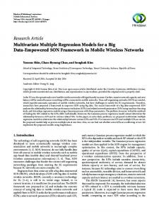
Figure 1: Thirty examples of true functions for Case a (left) and Case b (right)

5. Numerical Results and Practical Example We conducted Monte Carlo simulations to examine the effectiveness of the proposed procedures. We also applied the proposed modeling strategy to the analysis of spectrometric data. (1) Monte Carlo simulations We simulated n sets of a functional predictor and double responses {(xα (t), yα ); α = 1, . . . , n, t ∈ [0, 1]}, where yα = (yα1 , yα2 )0 , yαk = gk (uα ) + εαk , α = 1, . . . , n, k = 1, 2, ∫ gk (uα ) = uα (t)βk (t)dt, εα = (εα1 , εα2 )0 ∼ N2 (0, Σ), ( ) ry21 ρry1 ry2 c = 0.05, 0.1, Σ = × c, ρry1 ry2 ry22 ρ = 0.5, 0.8, where ryk = maxα (gk (uα )) − minα (gk (uα )), and functional predictor xαi is assumed to be obtained by xαi = uα (tαi ) + εαi , εαi ∼

i = 1, . . . , 100,

2 N (0, σxα ),

σxα = 0.05rxα ,

Regression Modeling for Functional Data

321

here rxα = maxi (xαi ) − mini (xαi ). We assumed that uα (t) and βk (t) are given by (a)

uα (t) = a1 sin(πt) + a2 , t ∈ [0, 1] a1 ∼ U (0.5, 1), a2 ∼ β1 (t) = sin(πt),

N (1, 0.52 )

β2 (t) = cos(πt).

(b)

uα (t) = exp(a1 t) + a2 , t ∈ [−1, 1] a1 ∼ N (2, 0.32 ), a2 ∼ N (−3, 0.42 ), β1 (t) = exp(t) − 1,

β2 (t) = −t/2.

Examples of true functions for each case are shown in Figure 1. First, we transfer the discrete data {xαi ; α = 1, . . . , n, i = 1 . . . , N } to a functional data set {xα (t); α = 1, . . . , n}. The nonlinear function uα (t) expressed as a linear combination of Gaussian basis functions are estimated in two-stage procedure; position the centers and determine the dispersions first by k-means clustering algorithm, then estimate the weights using the regularization method. The tuning parameters contained in the model are selected by using the Bayesian model selection criterion GBIC, due to Konishi et al. (2004). In smoothing functional data, all individual data should be fitted by using the common basis functions. In other words, numbers of basis functions are fixed, even though the amount of smoothness imposed on a set of discrete data will differ from each other. The regularization method allows us to adjust individual differences by smoothing parameters. Next, we fitted the functional multivariate regression models to the obtained functional predictor and responses {(xα (t), yα ); α = 1, . . . , n, t ∈ [0, 1]}. We used four criteria described in the previous section for evaluating the estimated models and examined their effectiveness. We fitted the functional univariate regression models separately to {(xα (t), yα1 ); α = 1, . . . , n, t ∈ [0, 1]} and {(xα (t), yα2 ); α = 1, . . . , n, t ∈ [0, 1]} by using GBIC to evaluate functional univariate regression models. Fourier series are also compared as basis functions. For simplicity, the basis functions of predictors φm (t) and of coefficient functions ψm (t) are restricted to be common in this simulation study. ∑ In the tables, we use the notation AMSEk = α (gk (xα )− yˆαk )2 /n, mean(λk ), and SD(λk ) (k = 1, 2) to denote the average squared errors, the means, and the standard deviations of the regularization parameters, respectively, where yˆαk denote the fitted values of yαk . It may be seen from the tables that for almost all cases the GBICF M gives the lowest AMSEs and the most stable models in four model selection criteria. Furthermore, in all cases, the functional multivariate regression model minimized AMSEk more than functional univariate regression models. Moreover, the AMSEs of the functional multivariate regression model based on Gaussian basis functions are lower than those based on Fourier series.

322

H. Matsui, Y. Araki and S. Konishi Table 1: Simulation results for model (a) when n = 50

c = 0.05, ρ = 0.5

c = 0.05, ρ = 0.8

c = 0.1, ρ = 0.5

c = 0.1, ρ = 0.8

AMSE1 × 102 AMSE2 × 102 mean(λ1 ) mean(λ2 ) SD(λ1 ) SD(λ2 ) AMSE1 × 102 AMSE2 × 102 mean(λ1 ) mean(λ2 ) SD(λ1 ) SD(λ2 ) AMSE1 × 102 AMSE2 × 102 mean(λ1 ) mean(λ2 ) SD(λ1 ) SD(λ2 ) AMSE1 × 102 AMSE2 × 102 mean(λ1 ) mean(λ2 ) SD(λ1 ) SD(λ2 )

GBICF M 1.15 1.19 0.67 0.24 0.39 0.32 1.13 1.22 0.57 0.24 0.40 0.33 2.22 2.32 0.65 0.31 0.40 0.38 2.09 2.01 0.67 0.27 0.40 0.33

GICF M 1.33 1.36 2.38 0.73 2.07 1.14 1.10 1.83 3.89 2.62 1.51 1.90 2.46 2.74 2.55 1.04 2.10 1.66 2.02 2.79 3.93 2.27 1.49 1.99

mAICF M 1.32 1.38 1.43 0.39 1.82 0.93 1.28 1.33 1.47 0.45 1.85 0.98 2.62 2.71 1.79 0.73 2.07 1.54 2.30 2.22 1.89 0.52 2.01 1.11

GCVF M 1.27 1.38 1.96 0.62 1.93 1.06 1.21 1.36 2.51 1.20 1.87 1.42 2.46 2.63 2.04 1.04 2.01 1.70 2.23 2.17 2.79 1.10 1.99 1.42

Univariate 1.18 1.23 2.10 0.51 1.93 1.17 1.16 1.32 1.81 0.59 1.96 1.27 2.24 2.44 2.24 0.94 1.98 1.70 2.09 2.16 2.28 0.68 1.98 1.32

Fourier 1.32 1.30 0.11 0.24 0.19 0.30 1.21 1.34 0.06 0.33 0.06 0.37 2.64 2.46 0.12 0.42 0.23 0.40 2.39 2.29 0.13 0.34 0.24 0.38

Table 2: Simulation results for model (a) when n = 100 c = 0.05, ρ = 0.5

c = 0.05, ρ = 0.8

c = 0.1, ρ = 0.5

c = 0.1, ρ = 0.8

AMSE1 × 103 AMSE2 × 103 mean(λ1 ) mean(λ2 ) SD(λ1 ) SD(λ2 ) AMSE1 × 103 AMSE2 × 103 mean(λ1 ) mean(λ2 ) SD(λ1 ) SD(λ2 ) AMSE1 × 102 AMSE2 × 102 mean(λ1 ) mean(λ2 ) SD(λ1 ) SD(λ2 ) AMSE1 × 102 AMSE2 × 102 mean(λ1 ) mean(λ2 ) SD(λ1 ) SD(λ2 )

GBICF M 7.91 6.63 0.55 0.20 0.40 0.30 7.38 6.35 0.54 0.16 0.41 0.25 1.70 1.17 0.58 0.18 0.40 0.27 1.34 1.05 0.51 0.19 0.40 0.31

GICF M 9.09 7.51 2.48 0.77 2.07 1.44 8.07 7.50 3.68 1.43 1.56 1.56 1.96 1.39 2.63 0.66 2.06 1.37 1.44 1.22 3.69 1.52 1.61 1.75

mAICF M 8.79 7.28 1.40 0.45 1.86 1.17 8.18 6.95 1.39 0.22 1.83 0.52 1.94 1.34 1.60 0.43 2.04 1.17 1.49 1.15 1.22 0.49 1.77 1.26

GCVF M 8.86 7.01 1.63 0.64 1.89 1.19 7.98 7.26 2.14 0.97 1.99 1.33 1.91 1.28 1.72 0.58 1.96 1.24 1.42 1.16 2.13 1.18 1.88 1.60

Univariate 8.06 6.79 1.59 0.57 1.89 1.37 7.63 6.98 1.77 0.35 1.94 0.86 1.74 1.22 1.87 0.50 2.01 1.24 1.35 1.11 1.77 0.71 2.02 1.54

Fourier 8.47 7.10 0.03 0.10 0.02 0.13 8.47 7.24 0.03 0.12 0.02 0.21 1.98 1.34 0.06 0.24 0.14 0.34 1.63 1.27 0.05 0.19 0.11 0.30

Regression Modeling for Functional Data

323

Table 3: Simulation results for model (b) when n = 50 c = 0.05, ρ = 0.5

c = 0.05, ρ = 0.8

c = 0.1, ρ = 0.5

c = 0.1, ρ = 0.8

AMSE1 × 102 AMSE2 × 102 mean(λ1 ) mean(λ2 ) SD(λ1 ) SD(λ2 ) AMSE1 × 102 AMSE2 × 102 mean(λ1 ) mean(λ2 ) SD(λ1 ) SD(λ2 ) AMSE1 × 102 AMSE2 × 102 mean(λ1 ) mean(λ2 ) SD(λ1 ) SD(λ2 ) AMSE1 × 102 AMSE2 × 102 mean(λ1 ) mean(λ2 ) SD(λ1 ) SD(λ2 )

GBICF M 6.70 1.23 0.28 0.39 0.19 0.14 6.65 1.20 0.27 0.36 0.19 0.17 12.60 2.41 0.26 0.39 0.19 0.15 14.65 2.28 0.26 0.38 0.20 0.15

GICF M 8.91 1.34 3.60 3.57 1.69 1.89 8.72 1.24 4.01 3.97 1.39 1.62 13.88 2.52 3.59 3.49 1.76 1.90 16.48 2.25 3.97 4.02 1.51 1.52

mAICF M 7.50 1.31 0.87 1.27 1.57 1.66 7.53 1.27 0.78 1.29 1.44 1.80 14.69 2.66 1.08 1.60 1.79 1.92 16.65 2.50 1.18 1.73 1.84 2.05

GCVF M 7.40 1.32 0.66 3.73 1.22 1.53 6.99 1.28 0.79 3.62 1.20 1.66 14.53 2.48 0.87 3.94 1.64 1.45 15.34 2.37 0.89 4.00 1.48 1.51

Univariate 7.15 1.30 1.17 2.06 1.74 1.76 7.19 1.28 1.19 2.17 1.74 1.79 12.97 2.51 1.70 2.39 2.07 1.92 15.64 2.40 1.66 2.85 2.05 1.89

Fourier 7.21 1.43 0.55 0.07 0.45 0.11 7.19 1.29 0.53 0.05 0.46 0.05 12.99 2.86 0.64 0.17 0.46 0.26 15.69 2.52 0.61 0.15 0.46 0.28

Table 4: Simulation results for model (b) when n = 100 c = 0.05, ρ = 0.5

c = 0.05, ρ = 0.8

c = 0.1, ρ = 0.5

c = 0.1, ρ = 0.8

AMSE1 × 102 AMSE2 × 102 mean(λ1 ) mean(λ2 ) SD(λ1 ) SD(λ2 ) AMSE1 × 102 AMSE2 × 102 mean(λ1 ) mean(λ2 ) SD(λ1 ) SD(λ2 ) AMSE1 × 102 AMSE2 × 102 mean(λ1 ) mean(λ2 ) SD(λ1 ) SD(λ2 ) AMSE1 × 102 AMSE2 × 102 mean(λ1 ) mean(λ2 ) SD(λ1 ) SD(λ2 )

GBICF M 5.34 1.02 0.16 0.32 0.17 0.18 5.38 1.00 0.17 0.24 0.18 0.19 8.42 1.63 0.20 0.35 0.19 0.18 10.28 1.65 0.17 0.30 0.18 0.19

GICF M 7.34 1.14 2.71 2.79 1.97 2.15 7.70 1.13 3.53 3.81 1.65 1.75 11.14 1.79 3.66 2.72 1.71 2.18 13.34 1.75 4.28 3.76 1.11 1.79

mAICF M 5.92 1.03 0.46 0.61 1.13 1.20 5.93 1.02 0.49 0.48 1.20 1.17 9.13 1.72 0.66 1.02 1.45 1.67 11.37 1.71 0.55 1.10 1.32 1.69

GCVF M 5.70 1.15 0.32 2.89 0.75 1.89 5.56 1.11 0.57 3.24 1.03 1.91 8.88 1.76 0.29 3.35 0.73 1.79 10.94 1.79 0.55 2.98 1.10 2.03

Univariate 5.63 1.08 0.62 1.27 1.37 1.51 5.67 1.08 0.60 1.29 1.32 1.60 8.88 1.69 0.95 1.85 1.66 1.82 10.63 1.76 0.93 1.64 1.66 1.80

Fourier 6.10 0.98 0.30 0.02 0.40 0.01 6.05 0.95 0.27 0.02 0.39 0.01 8.58 1.63 0.43 0.04 0.46 0.10 11.01 1.65 0.40 0.02 0.46 0.03

324

H. Matsui, Y. Araki and S. Konishi

(2) Tecator spectra benchmark

0

20

40 60 Channel

80

(a)

100

Standardized absorbance −1 0 1 −2

2.6

2.8

Absorbance 3.0 3.2 3.4

Standardized absorbance −1.5 −1.0 −0.5 0.0 0.5 1.0

3.6

1.5

We applied the proposed modeling strategy to the analysis of spectrometric data2 . Near-infrared absorbance spectra of a meat sample are observed at equal intervals with 100 channels from the wavelength range of from 850 nm to 1,050 nm (Figure 2(a)). The spectra are associated with contents of the meat sample, such as moisture, fat, and protein. In this example, we predict the contents of the meat sample using these spectra. Rossi et al. (2005) approached this problem using a B-spline approximation and modeling based on Neural-Networks to predict the fat content. Here, we predict all three contents simultaneously using the proposed model, treating the spectra as functional data.

0

20

40 60 Channel

80

100

(b)

0

20

40 60 Channel

80

100

(c)

Figure 2: Five spectra from the Tecator benchmark. (a): Observed data. (b): Standardized data. (c): Smoothed data by Gaussian basis expansion.

From n = 215 observed samples, 172 samples were used as a training set for model estimatinon ad the remaining 43 samples were used as a test set. In this experiment, we performed two preprocessings. First, the spectra were standardized, that is, for each α = 1, . . . , n we converted the observed data xαi into xαi − x ¯α (s) , xαi = √∑ ¯α )2 i (xαi − x ∑ where x ¯α = i xαi /N and N = 100. The standardized data are shown in Figure 2(b). Second, functionalization based on Gaussian basis functions is performed for each spectrum α = 1, . . . , n to obtain a functional data set (Figure 2(c)). The number of basis functions and the value of the hyperparameter are selected as p = 30 and ν = 30 respectively, by using the GBIC. 2

Tecator dataset. Available on statlib: http://lib.stat.cmu.edu/datasets/tecator

Regression Modeling for Functional Data

325

In order to investigate the effectiveness of the proposed model, we prepared three different models and compared the results obtained using these models. The three models are as follows: (a) The functional multivariate regression model (proposed model) was fitted by the regularization method. The regularization parameters were selected by GBICF M described in the previous section. Since there are 5 tuning parameters containing three regularization parameters, the number of basis functions and a hyperparameter, we employed the simulated annealing method to determine these values. (b) The functional univariate regression model was fitted such that correlation among the contents was not taken into consideration. The regularization parameters are selected using GBIC (Konishi et al., 2004). (c) The multivariate linear regression model was fitted by treating the spectra not as a functional but rather as conventional discrete data. That is, Y = XB + E, εα i.i.d. ∼ NK (0, Σ), (s)

where X = (xαi )αi . A coefficient matrix B and a variance covariance matrix Σ are estimated by the regularization method. This modeling strategy corresponds to the ridge regression described by Frank and Friedman (1993). The MSEs of each method are shown in Table 5. As a result of test set, the proposed model minimizes the MSE of fat content. In addition, rather than the multivariate regression model for the discrete data, the multivariate regression model for functional data minimized the MSE. Figure 3 shows the coefficient functions of each content. This figure shows that a positive weight is placed on the moisture and protein contents, and a negative weight is placed on the fat content in 60 to 80 channels. This reveals that the spectra absorbance in this interval strongly contributes to the contents. Table 5: MSE on training set and test set

Functional multivariate regression Functional univariate regression Multivariate regression

Train 4.27 2.87 2.94

Test 3.52 3.97 4.00

2

beta(t)

−2

−10

−400

0

−5

0

beta(t)

4

5

400 200 0

beta(t)

6

H. Matsui, Y. Araki and S. Konishi

10

326

0

20

40

60

80

channel

100

0

20

40

60

channel

80

100

0

20

40

60

80

100

channel

Figure 3: Coefficient functions of each content. Right: Moisture, Center: Fat, and Left: Protein.

6. Conclusion We constructed multivariate regression models with multiple scalar responses and functional predictors based on Gaussian basis functions, considering the relationship among responses. We estimated the model by the regularized maximum likelihood method. We also derived model selection criteria based on an information-theoretic and Bayesian approach to evaluate the model estimated by the regularization method. The proposed method is applied to a benchmark in spectroscopy, comparing the results of prediction with those of functional univariate regression models and ordinary multivariate linear regression models. Consequently, the proposed model minimized the prediction error of fat content the most. Based on the results of the proposed model, it is effective to take the relationship of three contents into consideration. Future research should consider the construction of functional regression modeling strategies in which the response and predictive variables are surfaces. Acknowledgements The authors would like to thank the anonymous reviewers for their helpful comments and suggestions. Appendix A. Smoothing Techniques by Basis Expansion We consider here that individual data should be considered to have a functional form in nature even though the data are usually observed discretely. In addition, those discrete raw data that are supposed to have functional form may contain observational error. Therefore, converting raw data into underlying smooth

Regression Modeling for Functional Data

327

functional form requires efficient smoothing techniques. We use Gaussian basis function expansion along with the technique of regularization. Suppose we have n observations x1 , . . . , xn , where each xα (α = 1, . . . , n) has Nα points xα1 , . . . , xαNα at times tα1 , . . . , tαNα , respectively. Then, we assume that the relationships between {tα1 , . . . , tαNα ; tαi ∈ T ⊂ R, i = 1, . . . , Nα } and {xα1 , . . . , xαNα } (α = 1, . . . , n) are given by following regression models: xαi = uα (tαi ) + εαi ,

i = 1, . . . , Nα ,

(A.1)

where uα (t) are unknown smooth functions and εαi are independently normally 2 . We assume that u (t) are expressed distributed with mean 0 and variance σxα α by linear combinations of basis functions uα (t) =

p ∑

wαj φj (t) = wα0 φ(t),

j=1

(t))0

where φ(t) = (φ1 (t), . . . , φp is a vector of basis functions and wα = (wα1 , . . . , wαp )0 are parameters that represent coefficients of φ(t). Here, we assume that φj (t) (j = 1, . . . , p) are Gaussian basis functions in the form given by ( ) ||t − cj ||2 φj (t) = exp − , 2νs2j where cj and s2j are parameters that represent centers and dispersions of each basis function, respectively. Ando et al. (2008) introduced a hyperparameter ν that also adjusts the dispersion of each basis function, enabling the estimated function to capture the structure in the data. The parameters cj and s2j are first determined by k-means clustering algorithms. The observational points {tα1 , . . . , tαNα } are divided into p clusters {C1 , . . . , Cp }, and then cj and s2j are determined by 1 ∑ 1 ∑ tαi , sˆ2j = (tαi − cˆj )2 , cˆj = Nj Nj tαi ∈Ch

tαi ∈Cj

respectively, where Nj = #{tαi ∈ Cj }. Thus, the regression model (A.1) has a probability density function { } 1 (xαi − wα0 φ(tαi ))2 2 f (xαi |tαi ; wα , σxα ) = √ exp − . 2 2 2σxα 2πσxα 2 are then estimated using the regularization The parameters wα and σxα method, which maximizes the following regularized log-likelihood function: 2 lζα (wα , σxα )=

Nα ∑ i=1

2 log f (xαi |tαi ; wα , σxα )−

N α ζα 0 wα Ωwα , 2

328

H. Matsui, Y. Araki and S. Konishi

where ζα are regularization parameters that adjust the smoothness of the estimated function, and Ω is a p × p positive semi-definite matrix. The regularized 2 are given by maximum likelihood estimators w ˆ α and σ ˆxα 2 w ˆ α = (Φ0α Φα + Nα ζα σ ˆxα Ω)−1 Φ0α xα ,

2 = σ ˆxα

1 (xα − Φα w ˆ α )0 (xα − Φα w ˆ α ), Nα

respectively, where Φα = (φ(tα1 ), . . . , φ(tαNα ))0 and xα = (xα1 , . . . , xαNα )0 . The regularized maximum likelihood estimates based on the Gaussian basis functions depend on the regularization parameters ζα , the number of basis functions p, and the hyperparameter ν in the Gaussian basis functions. For the choice of these parameters, Konishi and Kitagawa (2008) summarize the use of some model selection criteria. The result of these criteria gives appropriate values ζα , p, and ν, and leads to appropriate estimates u ˆα (t). Therefore, we obtain functional data as follows: xα (t) = u ˆα (t) = w ˆ 0α φ(t). We use a set of functions {xα (t); t ∈ T , α = 1, . . . , n} instead of the observed data set {(tαi , xαi ); i = 1, . . . , Nα , α = 1, . . . , n}. Appendix B. Derivation of GBICF M The regularized log-likelihood function (3.1) is rewritten as n lΛ (B, Σ) = log f (Y |θ) − tr{(Λ ¯ B)0 Ω0 B} 2 [ { ]} n = log f (Y |θ) exp − tr{(Λ ¯ B)0 Ω0 B} 2 { } K [ n ] ∏ 0 exp − b(k) (Λ(k) ¯ Ω0 )b(k) , = log f (Y |θ) 2 k=1

where log f (Y |θ) = l(B, Σ). We set the prior density of θ as a product of K multivariate normal distribution, i.e.,

π(θ|Λ) =

K ∏ n k=1

η−γ 2

1

|Λ(k) ¯ Ω0 |+2 (2π)

η−γ 2

[ n ] exp − b0(k) (Λ(k) ¯ Ω0 )b(k) . 2

(B.1)

The marginal likelihood of Y given θ with prior distribution (B.1) can then be

Regression Modeling for Functional Data

expressed as

329

∫ p(Y |Λ) = ∫ = ∫ =

f (Y |θ)π(θ|Λ)dθ [ ] 1 exp n × log{f (Y |θ)π(θ|Λ)} dθ n exp {nq(θ|Λ)} dθ,

(B.2)

where q(θ|Λ) = log{f (Y |θ)π(θ|Λ)}/n. A Taylor series expansion of q(θ|Λ) around ˆθ, the RMLE of θ, is given by 1 q(θ|Λ) = q(ˆθ|Λ) − (θ − ˆθ)0 RΛ (ˆθ)(θ − ˆθ) + · · · 2

(B.3)

since ∂q(ˆθ|Λ)/∂θ = 0. Substituting (B.3) into (B.2), we obtain the following Laplace approximation }] [ { ∫ ∫ 1 0 ˆ ˆ ˆ ˆ dθ exp {nq(θ|Λ)} dθ = exp n q(θ|Λ) − (θ − θ) RΛ (θ)(θ − θ) + · · · 2 ∫ { } { n } ≈ exp nq(ˆθ|Λ) exp − (θ − ˆθ)0 RΛ (ˆθ)(θ − ˆθ) dθ 2 (2π)

= n

Kη+r 2

Kη+r 2 1

|RΛ (θ)| 2

exp {nq(θ|Λ)} .

Therefore, the GBIC evaluating the functional multivariate regression model estimated by the regularized maximum likelihood method is given by {∫ } −2 log p(Y |Λ) = −2 log f (Y |θ)π(θ|Λ)dθ ˆ Σ) ˆ + ntr{(Λ ¯ B) ˆ 0 Ω0 B} ˆ + (r + Kγ) log n − (r + Kγ) log(2π) ≈ −2l(B, −

K ∑

log |Λ(k) ¯ Ω0 |+ + log |RΛ (ˆθ)|.

k=1

References Akaike, H. (1973). Information theory and an extension of the maximum likelihood principle. 2nd International Symposium on Information Theory (Edited by Petrov, B. N. and Csaki, F.). Akademiai Kiado, Budapest, 267-281. Akaike, H. (1974). A new look at the statistical model identification. IEEE Trans. Autom. Contr. AC-19 716-723.

330

H. Matsui, Y. Araki and S. Konishi

Ando, T., Konishi, S. and Imoto, S. (2008). Nonlinear regression modeling via regularized radial basis function networks. To appear in J. Stat. Plan. Infer. Araki, Y., Konishi, S., Kawano, S. and Matsui, H. (2007). Functional Regression Modeling via Regularized Gaussian Basis Expansions. To appear in Ann. Inst. Statist. Math. Cardot, H., Ferraty, F. and Sarda, P. (2003). Spline estimators for the functional linear model. Stat. Sinica 13, 571-591. Craven, P. and Wahba, G. (1979). Smoothing noisy data with spline functions: Estimating the correct degree of smoothing by the method of generalized cross validation. Numer. Math. 31, 317-403. Ferraty, F. and Vieu, P. (2006). Nonparametric Functional Data Analysis. Springer. Frank, I. and Friedman, J. H. (1993). A statistical view of some chemometrics regression tools. Technometrics 35, 109-148. Goutis, C. (1998). Second-derivative functional regression with applications to near infra-red spectroscopy. J. Roy. Statist. Soc. Ser. B 60, 103-114. Hastie, T. and Tibshirani, R. (1990). Generalized Additive Models. Chapman and Hall. Imoto, S. and Konishi, S. (2003). Selection of smoothing parameters in B-spline nonparametric regression models using information criteria, Ann. Inst. Statist. Math 55, 671-687. James, G. M. (2002). Generalized linear models with functional predictor variables. J. Roy. Statist. Soc. Ser. B 64, 411-432. Konishi, S., Ando, T. and Imoto, S. (2004). Bayesian information criteria and smoothing parameter selection in radial basis function network. Biometrika 91(1), 27-43. Konishi, S. and Kitagawa, G. (1996). Generalised information criteria in model selection. Biometrika 83, 875-890. Konishi, S. and Kitagawa, G. (2008). Information Criteria and Statistical Modeling. Springer. M¨ uller, H. G. and Stadtm¨ uller, U. (2005). Generalized functional linear models. Ann. Statist. 33, 774-805. Ramsay, J. O. and Silverman, B. W. (2002). Applied Functional Data Analysis. Springer. Ramsay, J.O. and Silverman, B.W. (2005). Functional Data Analysis Second Edition. Springer. Rossi, F., Delannay, N., Conan-Guez, B. and Verleysen, M. (2005). Representation of functional data in neural networks, Neurocomputing 64, 183-210. Schwarz, G. (1978). Estimating the dimension of a model. Ann. Statist. 6, 461-464.

Regression Modeling for Functional Data Received January 31, 2008 ; accepted May 4, 2008.

Hidetoshi Matsui Graduate School of Mathematics Kyushu University 6-10-1 Hakozaki, Higasi-ku, Fukuoka 812-8581, Japan [email protected] Yuko Araki Biostatistics Center Kurume University 67 Asahi-Machi, Kurume, Fukuoka 830-0011, Japan araki [email protected] Sadanori Konishi Faculty of Mathematics Kyushu University 6-10-1 Hakozaki, Higasi-ku, Fukuoka 812-8581, Japan [email protected]

331