39. ,134. ,248. 98,492. 40. ,122. ,226. 98,718. 41. ,110. ,204. 98,922. 42. 9,347E-02. ,173. 99,095. 43. 8,467E-02. ,157. 99,252. 44. 7,501E-02. ,139. 99,391. 45.
Hacettepe Journal of Mathematics and Statistics Volume 32 (2003), 75 – 90
MULTIVARIATE REPEATED MEASURES EXPERIMENT AND AN APPLICATION Zeynep Filiz∗
Received 17. 01. 2003 : Accepted 04. 03. 2003
Abstract In this study, an effective analysis approach for factorial experiments with repeated measurements involving m dependent variables is considered. This approach is applied to data concerning the students of the Faculty of Arts and Sciences, Osmangazi University, in order to determine whether time and department effects exist. In conclusion, it was determined that the benefits that students gain from university life do not differ due to department or department × time interaction, but time (semester) makes a change in the dependent variables. Keywords: Multivariate repeated measures experiment, Multivariate sphericity, Doubly multivariate model analysis, Multivariate mixed model analysis, Adjusted multivariate mixed model analysis
1. Introduction In this study, we will investigate the change in the benefits of university life during the first two years by defining the components of benefits. We will try to point out the expected change in the benefits that students gain from university life over time. The specific purpose of this study is to determine whether there is a difference in the benefits gained from university life among departments or semesters (time) for the students of the Departments of Biology, Physics, Statistics, Chemistry, Mathematics, History and Turkish Language and Literature at the Faculty of Arts and Sciences, Osmangazi University. In order to highlight the benefits that students gain, a survey entitled “Measuring the benefits of university life from a student’s perspective” was carried out by the students of seven departments during the 1999 − 2000 and 2000 − 2001 academic years. As seen above, this research is a factorial experiment with two factors, one of which is time with repeated measurements. The collection and the analysis of data were carried out according to Split-Plot in a Completely Random Design. ∗ Osmangazi University, Faculty of Arts and Sciences, Department of Statistics, Eski¸sehir, Turkey
76
Z. Filiz
In the experiment, semester (time) is defined as a “repeated factor” since the surveys were filled out by each student at the end of the fall and spring semesters of 1999 − 2000 and the fall semester of the 2000 − 2001 academic year. Since it is also investigated whether the benefits differ between departments, the department factor is taken as a “group factor”. Observing the same subjects (students) for the same variables at the end of different semesters (time instances) provides the control of the heterogeneity of the subjects and the differences between the individuals. Using the same subjects instead of independent ones at each observation decreases the within-subject errors. The multivariate analysis of factorial experiments with two factors, one of which is repeated, has been an important subject in the fields of psychology and education. In this study, we first give a theoretical approach using significance tests for factorial experiments with m = 3 dependent variables and two factors one of which is time involving repeated measurements, and then we investigate effective test techniques (Filiz, [3]).
2. Determining the appropriate test technique for multivariate analysis of variance involving repeated measurements There are two models (methods of analysis) to test the significance of multivariate repeated measurements: Doubly Multivariate Model Analysis and Multivariate Mixed Model Analysis (Boik, [2] and Schutz & Gessaroli, [10]). 2.1. The Doubly Multivariate Model Analysis. The linear model for repeated measurements of n subjects with m dependent variables is defined as follows: (2.1)
Y = θX + ξ,
where Y : mq × n is the response matrix, θ : mq × p is a matrix of parameters, X : p × n is the between groups design matrix having rank(X) = r ≤ p, and ξ : mq × n is a matrix of random errors. The k-th column of Y represents the mq dimensional response from the k-th subject. The responses are ordered within each column according to time and within time according to the dependent variable. The hypothesis is expressed as below: (2.2)
H0 : (C 0 ⊗ Im )θF = 0,
where C : q × a has rank(C) = a and F : p × s has rank(F ) = s. The columns of C consist of the coefficients of a linear functions of the q time periods. The columns of F consist of the coefficients of s estimable between group functions. To test the null hypothesis in Equation (2.2), we assume the following: (2.3) (2.4)
vec(ξ) ∼ Nnmq [0, (In ⊗ Ω)] 0
(C ⊗ Im )Y = (C0 ⊗ Im )θX + (C0 ⊗ Im )ξ
Assuming (2.3) and (2.4), the general test statistics for H0 in (2.2) is the characteristic root function of E −1 H. To test H0 in Equation (2.2), Wilks’ Lambda (Λ) criterion (Morrison, [9] and Keselman et al., [8]) defined below is used (2.5)
Λ = |E| / |E + H| .
Multivariate Repeated Measures Experiment
77
The error (within-groups) matrix (E) and the hypothesis (between-groups) matrix (H) are defined as follows: 0
(2.6)
E = (C ⊗ Im ) Y [In − X 0 (XX 0 )¯X]Y 0 (C ⊗ Im )
(2.7)
H = (C0 ⊗ Im )Y X 0 (XX 0 )¯F [F 0 (XX 0 )¯F ]−1 F 0 (XX 0 )¯XY 0 (C ⊗ Im ).
Both the matrices E and H have the Wishart distribution with the parameters calculated as below: (2.8)
E ∼ Wma [(n − r), Σ, 0]
(2.9)
H ∼ Wma [s, Σ, Ξ]
(2.10)
Σ = (C0 ⊗ Im )Ω(C ⊗ Im )
(2.11)
Φ = (C0 ⊗ Im )θF [F 0 (XX 0 )¯F ]−1 F 0 θ0 (C ⊗ Im )
(2.12)
Ξ = Σ−1 Φ
In order to find the p-value corresponding to Wilks’ Lambda (Λ) criterion, the transformed F value of Rao is calculated as below (Boik, [1]): v2 (2.13) F = (Λ−z − 1)( ) ∼ F (v1 , v2 ), v1 where Λ = |E| / |E + H| ½ 2 ¾1/2 d + m21 − 5 z= (m1 d)2 − 4 v1 = m 1 d 1 1 v2 = z −1 [m2 − (d − m1 + 1)] − (m1 d − 2). 2 2 Here, d is the product of the dimension of the error matrix (E) and that of the between groups matrix (H), (d = ma). m1 and m2 are the degrees of freedom of H and E respectively (m1 = s, m2 = n − r). The calculated F -sample value is compared with that of the F -table value, with v1 and v2 degrees of freedom at the α significance level. If the sample F value exceeds the critical F value, or the p-value corresponding to the sample F value is smaller than α, the null hypothesis H0 is rejected. 2.2. The Multivariate Mixed Model Analysis. In order to apply Multivariate Mixed Model Analysis, the elements of the linear model are redefined by making use of the linear model in Equation (2.1) and the reduced model in Equation (2.3). Here, we denote by Yk∗ the m × q matrix corresponding to the k-th subject’s response in the Y response matrix. The rows of this matrix correspond to the dependent variables, whereas the columns represent time (semester). Thus the adjusted response matrix can be written as follows £ ¤ (2.14) Y ∗ = Y1∗ Y2∗ · · · Yk∗ · · · Yn∗ m×qn . The coefficient (parameter) matrix θ and the error matrix ξ are recalculated according to the requirements of Multivariate Mixed Model Analysis as follows: (2.15)
θ ∗ = ( θ1∗
···
θi∗
···
θk∗ ) and ξ ∗ = ( ξ1∗
···
ξj∗
Then, we can rewrite the linear model in Equation (2.1) as follows : (2.16)
Y ∗ = θ∗ (X ⊗ Iq ) + ξ ∗ ,
whereas the reduced linear model is the following: (2.17)
Y ∗ (In ⊗ C) = θ ∗ (X ⊗ C) + ξ ∗ (In ⊗ C).
···
ξn∗ ).
78
Z. Filiz
Assuming the linear model in Equation (2.3), the reduced model in Equation (2.17) and the multivariate sphericity, the null hypothesis that the effects of groups (departments), time (semester) and group×time interaction do not exist is expressed as follows: (2.18)
H0 : θ∗ (F ⊗ C) = 0.
To test H0 , the characteristic root functions of E ∗−1 H ∗ are used. The generalized Λ criterion which is based on probability ratio was proposed by Wilks and can be written as follows: (2.19)
Λ = |E ∗ | / |E ∗ + H ∗ |
Here, the error matrix E ∗ and the between-groups (hypothesis) matrix H ∗ are defined below: ©£ ¤ ª 0 (2.20) E ∗ = Y ∗ In − X 0 (XX 0 )¯X ⊗ CC 0 Y ∗ n o 0 £ ¤−1 0 (2.21) H ∗ = Y ∗ X 0 (XX 0 )¯F F 0 (XX 0 )¯F F (XX 0 )¯X ⊗ CC 0 Y ∗
In order to use Rao’s F estimate in this method, we replace in Equation (2.13) the error matrix E by E ∗ and the between-groups matrix H by H ∗ . If multivariate sphericity Σ = (Ia ⊗ γ) is satisfied, the error matrix E ∗ and betweengroups (hypothesis) matrix H ∗ are distributed as follows: (2.22)
E ∗ ∼ Wm [m2 = (n − r)a, γ, 0]
(2.23)
H ∗ ∼ Wm [m1 = sa, γ, Ξ∗ )
where, the parameters of the distribution are calculated in the following way: Σ = (C 0 ⊗ Im )Ω(C ⊗ Im ) a
1 X γ=( ) Σii a i=1
(2.24)
£ ¤−1 Φ = (C 0 ⊗ Im )θF F 0 (XX 0 )¯F
a X © ª 0 Ξ∗ = γ −1 θ∗ F [F 0 (XX 0 )¯F ]−1 F 0 ⊗ CC 0 θ∗ = γ −1 Φii i=1
Here, the parameters are defined as below: Σii and Φii represent the i’th m × m diagonal blocks of Σ and Φ respectively. We have also the following relations: d = m, m1 = sa and m2 = (n − r)a. 2.3. Testing the Validity Assumptions of Multivariate Analysis Techniques. As explained above, Doubly Multivariate Model Analysis and Multivariate Mixed Model Analysis are used to test (2.2) and (2.18) respectively: H0 : (C0 ⊗ Im )θF = 0, and H0 : θ∗ (F ⊗ C) = 0. These two analyses require the following two assumptions to be verified: (1) Multivariate normality assumption of errors (2.25)
vec(ξj ) ∼ N (0, Ωj ).
(2) The homogeneity assumption of the variance-covariance matrix: (2.26)
(C 0 ⊗ Im )Ωj (C ⊗ Im ) = (C 0 ⊗ Im )Ωj 0 (C ⊗ Im ) ∀ j, 0
Multivariate Repeated Measures Experiment
79
The multivariate normality and the homogeneity assumptions are necessary and sufficient assumption for the validity of Doubly Multivariate Model Analysis. If Equation (2.3) is satisfied, it follows that the multivariate normality of errors and the homogeneity of the variance-covariance matrix are satisfied. In addition to the above matrices, the error matrix E ∗ and the between groups matrix H should be independently distributed as Wishart matrices. To satisfy the independence of the matrices E ∗ and H ∗ , the error in Equation (2.3) must have a multivariate normal distribution (Timm, [12]; Wang, [13]). If additionally Equation (2.3) is satisfied, the multivariate sphericity Σ = (Ia ⊗ γ) assumption is a necessary and sufficient condition for the error matrix E ∗ and between-groups (hypothesis) matrix H ∗ to have the Wishart distribution. ∗
The null hypothesis is expressed as follows: (2.27)
H0 : Σ = (Ia ⊗ γ).
Here, Σ is calculated as Σ = (C 0 ⊗ Im )Ω(C ⊗ Im ). To test the null hypothesis above, the test statistics which is also in the form of a probability ratio was proposed by Thomas [11] as follows: ¯ ¯na/2 a ¯ ¯ ¯ −1 X ¯ n/2 (2.28) λ = |E| ÷ ¯a Eii ¯ ¯ ¯ i=1
Here, −2 ln(λ) asymptotically has a χ2 distribution with f degrees of freedom (-2 ln(λ) ∼ χ2f ). The degree of freedom f is calculated as follows: (2.29)
f=
m(a − 1)(ma + m + 1) . 2
2.4. Adjusted Multivariate Mixed Model Analysis for Multivariate Non-sphericity. If the sphericity assumption is not satisfied, a correction factor similar to the one proposed by Box was used by Boik [1] for Multivariate Mixed Model Analysis. The correction factor is as follows:
(2.30)
a a P P Σii )]2 Σii )2 ] + [tr( tr[( i=1 i=1 ) ε= ( a P a £ ¤ P 2 2 a (trΣij ) + tr(Σij ) i=1 j=1
As in Multivariate Mixed Model Analysis, the null hypothesis that the effects of group (department), time (semester) and groups × time interactions are zero in Adjusted Multivariate Mixed Model Analysis is H0 : (C0 ⊗ Im )θF = 0. In the same manner, the characteristic root functions of E ∗−1 H ∗ are used to test H0 . Wilks’ lambda Λ criterion is used to test H0 . Λ is based on the generalized probability ratio: Λ = |E ∗ | / |E ∗ + H ∗ | Here, the error matrix E ∗ and the between-groups (hypothesis) matrix H ∗ are calculated as in Multivariate Mixed Model Analysis. The parameters are merely multiplied by the correction factor when the sphericity assumption is not satisfied. In this method, the error matrix E ∗ ∼ Wm [ε(n − r)a, γ, 0] and between-groups (hypothesis) matrix H ∗ ∼ Wm [εa(s + 2aεδ), γ, Ξ∗ ] have the Wishart distribution with the
80
Z. Filiz
following parameters: γ=(
a 1 X Σii ) aε i=1
Ξ∗ = aε(
a X
Σii )−1
i=1
δ1 δ= δ2 tr(
a P
−
Φii − 2(aε)2 δIm
i=1
Σii )tr(
i=1
δ1 =
a X
a P
Φii ) + tr[(
i=1
a a X X
a P
i=1
aε
Σii )(
a P
Φii )]
i=1
[tr(Σij )tr(Φij ) + tr(Σij Φij )]
i=1 j=1
(2.31)
δ2 = tr(
a X
Σii )2 + [tr(
i=1
a X
Σii )]2
i=1
To find the p-value corresponding to Wilks’ Lambda Λ criterion, the transformation value F of Rao is found as below (Boik, [1]): v2 F = (Λ−z − 1)( ) ∼ F (v1 , v2 ) v1 Λ = |E ∗ | / |E ∗ + H ∗ | ¾1/2 ½ 2 d + m21 − 5 z= (m1 d)2 − 4 v1 = m 1 d ¸ · 1 1 v2 = z −1 m2 − (d − m1 + 1) − (m1 d − 2) 2 2 d=m m1 = εsa (2.32)
m2 = ε(n − r)a
The sample F value is compared with the Fα;v1 ,v2 distribution. If the sample F value exceeds the critical table value, or the p-value is less than α, then the null hypothesis is rejected at the specified significance level.
3. The Analysis of Benefits gained from University Life The data are obtained from surveys completed by 70 students in 7 Departments of the Faculty of Arts and Sciences after the fall and spring semesters of the 1999 − 2000 academic year, and after the fall semester of the 2000 − 2001 academic year. In order to decrease the number of the dependent variables (m = 3), a principal component analysis was done. In order to solve the conceptual significance problem at this step, Cronbach’s α value was determined for the internal validity of the survey. The Cronbach’s α value was calculated as 0.7174. We have obtained 3 components labled “Gratitude, Importance, Socialization” as the result of the factor analysis. 3.1. Application of Doubly Multivariate Model Analysis. The number of levels in factor B (time) is (q = 3), whereas the number of levels in factor A (department) is (p = 7). The number of students in each department is ni = 10, with a total of 70
Multivariate Repeated Measures Experiment
81
students (n = 70). The data for each group (department) is assumed to come from sublevels with a multivariate normal distribution. The general statement of H0 in Doubly Multivariate Model Analysis is as follows: H0 : (C0 ⊗ I3 )θF = 0. To test the null hypothesis that the effect of department, time and department × time interaction are zero, we have determined the matrices C and F . After determining the other parameters, the error and between- groups (hypothesis) matrices of Rao’s F transformation, we have obtained the results of Doubly Multivariate Model Analysis which we present in Table 1. Table 1. Results of the Doubly Multivariate Model Analysis Source of
Rank of C Rank of F Λ = |E| / |E + H|
Variation
(a)
(s)
Department
1
6
0,7276
F
v1
v2
1,1437 18 173,019
Time (Semester)
2
1
0,9999
9,6670
Department × Time
2
6
0,5826
0,9364 36 257,457
6
58,000
As seen in Table 1, there is no difference between department effects and department × time interaction effects at a 5% significance level. The different departments do not affect the benefits of university life, and neither does the department × time interaction. But time (semester) does cause a change in the dependent variables (Fh = 9, 667 > F0,05;6,58 = 2, 25), so there is a difference between the benefits of university life as time passes. 3.2. Searching for Applicability of Multivariate Mixed Model Analysis. In order to test the hypothesis that the within-subject effects (time and time × department) are zero, we tried to find out whether the multivariate sphericity assumption is satisfied or not. The null hypothesis that the multivariate sphericity is satisfied is expressed as follows: H0 : Σ = (Ia ⊗ γ). ¯ ¯na/2 a ¯ −1 P ¯ ¯ To test the hypothesis above, we used the test statistics, λ = |E| / ¯a Eii ¯¯ . i=1 2 The test statistics is found as −2ln(λ) = 51.693 > χ0,05;15 = 24, 9958. Then, we reject the hypothesis at the 5% significance level, so we cannot use Multivariate Mixed Model Analysis. However, to verify the results we obtained from Doubly Multivariate Model Analysis, we will also use another test. n/2
3.3. Application of Adjusted Multivariate Mixed Model Analysis. Since the multivariate sphericity assumption is not satisfied, Adjusted Multivariate Mixed Model Analysis is an appropriate technique to test that the main effect of time, and the interaction effect of time and department, are zero. However, the degrees of freedom of the error and hypothesis matrices should be corrected. The correction factor is calculated as follows: a a P b ii )2 ] + [tr( P Σ b ii )]2 tr[( Σ i=1 i=1 ) = 0, 956. εb = ( i a P a h P 2 2 c b a (trΣij ) + tr(Σ ij ) i=1 j=1
82
Z. Filiz
The null hypothesis that the main and interaction effects are zero is expressed as: H0 : θ∗ (F ⊗ C) = 0. We have now found the matrices C and F , the error and hypothesis matrices of Rao’s F transformation and other the parameters. We present the results of the Adjusted Multivariate Mixed Model Analysis in Table 2. We also found that there is no difference between the main effects of department and of the department × time interaction effect at the 5% significance level. However the main effect of time is significant ( Fh = 40, 102 > F0,05;6,230 = 2, 1 ). Table 2. Results of the Adjusted Multivariate Mixed Model Analysis Source of
Rank of C Rank of F
Λ= ∗
∗
F
v1
v2
18
29,863
∗
Variation
(a)
(s)
|E | / |E + H |
Department
1
6
0,7391
1,106
Time (Semester)
2
1
0,9998
40,102 5,7336 229,903
Department × Time
2
6
0,7705
0,940 34,4016 350,100
4. Conclusion We have firstly applied Reliability Analysis to the survey data and carried out a Principal Component and Factor Analysis; the results are given in the Appendix. Then, we have used Doubly Multivariate Model Analysis, which only requires multivariate normality. We concluded that only the time (semester) factor is effective at the 5% significance level. Secondly we tested whether the multivariate sphericity assumption is satisfied. Since it was not satisfied, we used Adjusted Multivariate Mixed Model Analysis instead of Multivariate Mixed Model Analysis. We have also found that only the time effect is significant. The benefits that students gain from university life at Osmangazi University are only dependent on time, and not on the student’s Department. That is, the time spent at the university affects the benefits the students gain, which are categorized as “Gratitude, Importance and Socialization” at the 5% significance level. In conclusion, the F -value used in the Adjusted Multivariate Mixed Model Analysis (for time) is larger than that of the Doubly Multivariate Model Analysis. So, the Adjusted Multivariate Model Analysis seems to be more effective.
5. Appendix RELIABILITY ****** Method 2 (covariance matrix) will be used for this analysis ****** R E L I A B I L I T Y A N A L Y S I S - S C A L E (A L P H A) * * * Warning * * * Determinant of matrix is close to zero: 2, 584E − 18 Statistics based on inverse matrix for scale ALPHA are meaningless and printed as . N of Cases = 70,0
Multivariate Repeated Measures Experiment
83
R E L I A B I L I T Y A N A L Y S I S - S C A L E (A L P H A) Item-total Statistics
VAR00001 VAR00002 VAR00006 VAR00007 VAR00009 VAR00011 VAR00013 VAR00015 VAR00018 VAR00021 VAR00022 VAR00023 VAR00025 VAR00026 VAR00027 VAR00028 VAR00029 VAR00030 VAR00031 VAR00032 VAR00033 VAR00034 VAR00035 VAR00036 VAR00037 VAR00038 VAR00039 VAR00040 VAR00041 VAR00042 VAR00043 VAR00044 VAR00045 VAR00046 VAR00047 VAR00048 VAR00049
Scale Mean if Item Deleted 122,6729 131,9086 133,8543 132,6157 134,8371 128,3971 129,1229 131,5371 133,2371 132,6371 132,2943 132,4514 132,7229 132,3086 132,7514 133,5800 132,8800 133,5943 132,9943 132,8657 131,3800 133,0943 131,4800 133,6943 132,4086 132,0800 131,7371 133,4229 131,9371 133,8229 132,2800 133,7371 132,4657 133,7657 132,2943 133,6371 132,1371
Scale Variance if Item Deleted 745,0571 836,5956 881,4240 871,3608 896,5974 847,6594 810,0293 889,2389 896,2456 881,3111 875,9307 887,0727 884,2885 897,5567 886,5269 896,7294 897,4996 894,6661 891,3490 901,4698 884,5532 895,4646 868,4515 897,3846 883,9738 883,7773 883,0760 894,7183 875,6783 892,1200 870,9506 893,2499 863,2072 895,3368 860,1945 898,1922 876,3328
Corrected ItemTotal Correlation ,1245 ,1836 ,1868 ,1069 ,3084 ,0734 ,1614 ,2014 ,1711 ,4751 ,4387 ,3440 ,3796 ,1056 ,3041 ,1730 ,1054 ,1886 ,1814 ,0273 ,2574 ,1206 ,4201 ,1745 ,2905 ,2566 ,2754 ,1795 ,3712 ,4351 ,3986 ,2482 ,5503 ,1992 ,5624 ,1692 ,3924
Squared Multiple Correlation . . . . . . . . . . . . . . . . . . . . . . . . . . . . . . . . . . . . .
Alpha if Item Deleted ,7816 ,7179 ,7134 ,7199 ,7150 ,7368 ,7303 ,7139 ,7154 ,7103 ,7089 ,7123 ,7114 ,7163 ,7124 ,7154 ,7163 ,7149 ,7145 ,7182 ,7124 ,7159 ,7072 ,7156 ,7119 ,7123 ,7119 ,7150 ,7094 ,7135 ,7080 ,7143 ,7048 ,7150 ,7039 ,7158 ,7093
84
Z. Filiz
Item-total Statistics (Continued)
VAR00051 VAR00052 VAR00053 VAR00054 VAR00055 VAR00056 VAR00057 VAR00058 VAR00059 VAR00060 VAR00061 VAR00062 VAR00063 VAR00064 VAR00065 VAR00066 VAR00067
Scale Mean if Item Deleted 131,8086 133,3229 132,0943 133,7943 132,2229 133,3943 132,6371 133,8086 132,6800 133,7514 132,5514 133,7514 132,5371 133,7657 132,6943 133,7086 132,2943
Scale Variance if Item Deleted 871,9321 882,6635 861,1197 890,0017 872,0000 795,2376 876,6386 891,3988 872,4219 887,1269 868,3217 890,3878 876,6563 890,0034 868,8513 889,0020 864,1365
Corrected ItemTotal Correlation ,4481 ,2165 ,5792 ,4637 ,3958 ,4406 ,3662 ,4513 ,4357 ,4094 ,4697 ,3324 ,3495 ,4751 ,5349 ,3936 ,5296
Squared Multiple Correlation . . . . . . . . . . . . . . . . .
Alpha if Item Deleted ,7078 ,7127 ,7041 ,7128 ,7083 ,6948 ,7096 ,7133 ,7080 ,7121 ,7067 ,7132 ,7098 ,7128 ,7065 ,7127 ,7052
Analysis of Variance Source of Variation Between People Within People Between Measures Residual Nonadditivity Balance Total Grand Mean
Sum of Sq. 1156,5199 28619,4600 11295,1568 17324,3032 1167,4468 16156,8565 29775,9799 2,5002
DF 69 3710 53 3657 1 3656 3779 -
Mean Square 16,7612 7,7141 213,1162 4,7373 1167,4468 4,4193 7,8793 -
F 44,9868 264,1718 -
Tukey estimate of power to which observations must be raised to achieve additivity = -,4531 Hotelling’s T-Squared = 5262,7067 F = 24,4643 Prob. = ,0000 Degrees of Freedom: Numerator = 53 Denominator = 17 Reliability Coefficients 54 items Alpha = ,7174 Factor Analysis
Standardized item alpha = ,8969
Prob. ,0000 ,0000 -
Multivariate Repeated Measures Experiment
Communalities VAR00001 VAR00002 VAR00006 VAR00007 VAR00009 VAR000011 VAR000013 VAR000015 VAR000018 VAR000021 VAR000022 VAR000023 VAR000025 VAR000026 VAR000027 VAR000028 VAR000029 VAR000030 VAR000031 VAR000032 VAR000033 VAR000034 VAR000035 VAR000036 VAR000037 VAR000038 VAR000039 VAR000040 VAR000041 VAR000042 VAR000043 VAR000044 VAR000045 VAR000046 VAR000047 VAR000048 VAR000049 VAR000051 VAR000052 VAR000053 VAR000054 VAR000055 VAR000056 VAR000057 VAR000058 VAR000059 VAR000060 VAR000061 VAR000062 VAR000063 VAR000064 VAR000065 VAR000066 VAR000067
Initial 1,000 1,000 1,000 1,000 1,000 1,000 1,000 1,000 1,000 1,000 1,000 1,000 1,000 1,000 1,000 1,000 1,000 1,000 1,000 1,000 1,000 1,000 1,000 1,000 1,000 1,000 1,000 1,000 1,000 1,000 1,000 1,000 1,000 1,000 1,000 1,000 1,000 1,000 1,000 1,000 1,000 1,000 1,000 1,000 1,000 1,000 1,000 1,000 1,000 1,000 1,000 1,000 1,000 1,000
Extraction 8,542E-02 ,224 ,142 1,845E-02 ,119 5,481E-02 ,173 ,172 ,122 ,378 ,290 ,199 ,168 ,210 ,200 ,393 ,146 ,396 ,147 ,468 ,206 ,601 ,375 ,352 ,266 ,167 ,154 ,370 ,347 ,549 ,436 ,606 ,764 ,594 ,718 ,443 ,400 ,423 ,267 ,635 ,592 ,416 ,424 ,434 ,644 ,629 ,604 ,502 ,577 ,548 ,653 ,629 ,289 ,583
Extraction Method:
Principle Component Analysis
85
86
Z. Filiz
Total Variance Explained
Comp. 1 2 3 4 5 6 7 8 9 10 11 12 13 14 15 16 17 18 19 20 21 22 23 24 25 26 27 28 29 30 31 32 33 34 35 36 37 38 39 40 41 42 43 44 45 46 47 48 49 50 51 52 53 54
Initial Eigenvalues Total % Var Cum. % 9,988 18,496 18,496 6,645 12,305 30,800 3,673 6,802 37,603 2,685 4,972 42,575 2,653 4,913 47,488 2,171 4,021 51,509 2,107 3,902 55,410 1,958 3,626 59,036 1,925 3,565 62,601 1,812 3,356 65,978 1,499 2,775 68,733 1,351 2,502 71,235 1,270 2,352 73,587 1,192 2,208 75,795 1,122 2,078 77,872 1,055 1,953 79,826 ,954 1,766 81,592 ,851 1,577 83,168 ,817 1,513 84,681 ,751 1,390 86,071 ,666 1,233 87,304 ,621 1,150 88,455 ,601 1,113 89,568 ,507 ,938 90,506 ,489 ,906 91,412 ,422 ,782 92,194 ,391 ,725 92,918 ,364 ,673 93,592 ,355 ,658 94,250 ,336 ,622 94,872 ,318 ,589 95,461 ,277 ,514 95,975 ,251 ,464 96,439 ,235 ,435 96,875 ,231 ,428 97,303 ,205 ,380 97,683 ,159 ,295 97,978 ,143 ,265 98,244 ,134 ,248 98,492 ,122 ,226 98,718 ,110 ,204 98,922 9,347E-02 ,173 99,095 8,467E-02 ,157 99,252 7,501E-02 ,139 99,391 6,624E-02 ,123 99,514 5,502E-02 ,102 99,616 4,821E-02 8,928E-02 99,705 4,396E-02 8,141E-02 99,786 3,790E-02 7,018E-02 99,856 2,422E-02 4,486E-02 99,901 2,064E-02 3,823E-02 99,939 1,417E-02 2,624E-02 99,966 1,108E-02 2,052E-02 99,986 7,438E-03 1,377E-02 100,000 Extraction Method:
Extraction Sums of Squared Loadings Total % Var. Cum. % 9,988 18,496 18,496 6,645 12,305 30,800 3,673 6,802 37,603
Rotation Sums of Squared Loadings Total % Var. Cum. % 9,181 17,002 17,002 6,325 11,712 28,714 4,800 8,888 37,603
Principle Component Analysis
Multivariate Repeated Measures Experiment
87
Scree Plot 12
10
8
6
Eigenvalue
4
2
0 1
4
7
10 13 16 19 22 25 28 31 34 37 40 43 46 49 52
Component Number
Component Transformation Matrix Component
1
2
3
1
,914
,161
,372
2
-,280
,915
,291
3
,294
,370
-,881
Extraction Method: Principle Component Analysis. Rotation Method: Varimax with Kaiser Normalization.
Component Score Covariance Matrix Component
1
2
3
1
1,00
,000
,000
2
,000
1,000
,000
3
,000
,000
1,000
Extraction Method: Principle Component Analysis. Rotation Method: Varimax with Kaiser Normalization.
88
Z. Filiz
Component Matrix
VAR00045 VAR00047 VAR00065 VAR00053 VAR00067 VAR00059 VAR00061 VAR00043 VAR00063 VAR00057 VAR00041 VAR00055 VAR00051 VAR00049 VAR00035 VAR00021 VAR00037 VAR00022 VAR00023 VAR00027 VAR00025 VAR00015 VAR00039 VAR00009 VAR00031 VAR00029 VAR00011 VAR00044 VAR00046 VAR00042 VAR00034 VAR00048 VAR00040 VAR00036 VAR00032 VAR00028 VAR00056 VAR00060 VAR00030 VAR00064 VAR00052 VAR00066 VAR00006 VAR00038 VAR00018 VAR00001 VAR00062 VAR00054 VAR00058 VAR00002 VAR00013 VAR00026 VAR00033 VAR00007
1 ,830 ,809 ,774 ,742 ,720 ,708 ,685 ,635 ,613 ,594 ,575 ,572 ,569 ,560 ,542 ,515 ,477 ,472 ,425 ,407 ,398 ,396 ,391 ,323 ,310 ,274 ,168 ,163 ,112 ,300 2,235E-02 ,109 ,104 4,619E-02 -6,30E-02 ,146 ,245 ,386 ,105 ,417 ,157 ,279 5,788E-02 ,253 ,138 6,157E-02 ,329 ,387 ,416 ,203 ,196 ,304 ,279 5,491E-02
Extraction :
∗
Component 2 -,135 -,182 -,159 -,124 -,251 -,309 -,158 -,161 -,331 -,278 -,119 -,271 -6,11E-02 -,104 -,162 ,207 -,158 ,129 1,125E-02 4,333E-02 -5,11E-02 -,123 2,665E-02 -,122 -8,42E-02 -3,56E-02 -,163 ,742 ,706 ,669 ,656 ,650 ,573 ,562 ,557 ,554 ,538 ,509 ,500 ,493 ,487 ,384 ,371 ,319 ,315 ,262 ,275 ,343 ,439 -5,30E-02 1,214E-02 4,588E-02 -,202 6,069E-03
Rotated Component Matrix 3 ,239 ,173 -6,88E-02 ,262 3,637E-02 -,178 -8,42E-02 8,430E-02 -,249 -5,81E-02 5,165E-02 ,124 ,310 ,274 ,234 ,265 ,116 ,227 -,133 -,182 -8,38E-02 3,629E-03 -2,83E-02 -1,88E-02 ,210 ,264 3,442E-03 ,169 ,287 -,105 ,414 9,188E-02 ,176 ,185 ,393 ,255 -,272 -,443 ,367 -,487 7,601E-02 -,252 3,387E-02 -3,22E-02 6,509E-02 -,114 -,627 -,570 -,528 -,425 -,366 ,340 ,296 -,124
Principle Component Analysis.
VAR00045 VAR00047 VAR00053 VAR00067 VAR00065 VAR00059 VAR00043 VAR00061 VAR00055 VAR00051 VAR00049 VAR00035 VAR00057 VAR00063 VAR00041 VAR00037 VAR00021 VAR00022 VAR00033 VAR00015 VAR00031 VAR00026 VAR00025 VAR00023 VAR00039 VAR00029 VAR00009 VAR00011 VAR00046 VAR00044 VAR00034 VAR00048 VAR00032 VAR00028 VAR00042 VAR00030 VAR00040 VAR00036 VAR00052 VAR00006 VAR00018 VAR00038 VAR00001 VAR00062 VAR00058 VAR00054 VAR00064 VAR00060 VAR00056 VAR00066 VAR00002 VAR00013 VAR00027 VAR00007
Extraction : Rotation :
∗
3 components extracted
1 ,867 ,841 ,790 ,739 ,731 ,681 ,650 ,646 ,635 ,628 ,622 ,610 ,604 ,580 ,574 ,515 ,491 ,462 ,398 ,397 ,369 ,365 ,353 ,346 ,342 ,338 ,324 ,200 -1,06E-02 -9,48E-03 -4,15E-02 -5,52E-02 -9,80E-02 5,358E-02 5,628E-02 6,387E-02 -1,34E-02 -6,06E-02 2,939E-02 -4,09E-02 5,713E-02 ,132 -5,05E-02 3,908E-02 ,102 8,983E-02 ,100 7,995E-02 -6,96E-03 7,378E-02 7,511E-02 6,804E-02 ,306 1,204E-02
∗∗
Component 2 9,918E-02 2,760E-02 ,103 -,100 -4,58E-02 -,234 -,36E-02 -6,55E-02 -,110 ,150 9,663E-02 2,584E-02 -,180 -,296 3,334E-03 -2,45E-02 ,370 ,278 -3,02E-02 -4,75E-02 5,079E-02 ,217 -1,36E-02 2,958E-02 7,697E-02 ,109 -6,66E-02 -,121 ,771 ,768 ,756 ,646 ,645 ,624 ,622 ,611 ,606 ,590 ,499 ,361 ,334 ,321 ,208 7,301E-02 ,273 ,165 ,338 ,364 ,431 ,303 -,173 -9,28E-02 3,797E-02 -3,15E-02
∗∗
3 5,930E-02 9,554E-02 9,245E-03 ,163 ,303 ,331 ,115 ,283 2,536E-02 -7,90E-02 -6,26E-02 -5,13E-02 ,192 ,352 ,134 2,943E-02 1,876E-02 1,291E-02 -,215 ,108 -9,45E-02 -,173 ,207 ,279 ,178 -,141 ,101 1,195E-02 -6,03E-03 ,128 -,166 ,149 -,208 -9,28E-03 ,399 -,139 5,003E-02 1,721E-02 ,133 9,945E-02 8,552E-02 ,215 ,200 ,755 ,748 ,746 ,727 ,682 ,488 ,438 ,435 ,399 ,324 ,132
Principle Component Analysis.
Varimax with Kaiser Normalization.
Rotation converged in 5 iterations
Multivariate Repeated Measures Experiment
Component Score Coefficient Matrix
VAR00001 VAR00002 VAR00006 VAR00007 VAR00009 VAR00011 VAR00013 VAR00015 VAR00018 VAR00021 VAR00022 VAR00023 VAR00025 VAR00026 VAR00027 VAR00028 VAR00029 VAR00030 VAR00031 VAR00032 VAR00033 VAR00034 VAR00035 VAR00036 VAR00037 VAR00038 VAR00039 VAR00040 VAR00041 VAR00042 VAR00043 VAR00044 VAR00045 VAR00046 VAR00047 VAR00048 VAR00049 VAR00051 VAR00052 VAR00053 VAR00054 VAR00055 VAR00056 VAR00057 VAR00058 VAR00059 VAR00060 VAR00061 VAR00062 VAR00063 VAR00064 VAR00065 VAR00066 VAR00067
1 -,015 -,013 -,008 -,005 ,033 ,023 -,012 ,042 ,005 ,060 ,056 ,028 ,032 ,053 ,021 ,010 ,048 ,018 ,049 ,002 ,058 ,008 ,075 -,005 ,060 ,007 ,032 -,001 ,062 -,009 ,072 -,003 ,101 ,004 ,096 -,010 ,078 ,079 ,000 ,094 -,025 ,074 -,022 ,061 -,023 ,064 -,022 ,063 -,032 ,050 -,022 ,072 -,011 ,079
Component 2 ,026 -,047 ,055 -,011 -,013 -,019 -,032 -,010 ,052 ,063 ,048 -,005 -,009 ,045 -,006 ,104 ,026 ,108 ,015 ,115 ,007 ,132 ,010 ,097 -,002 ,045 ,007 ,098 -,002 ,086 -,003 ,122 ,019 ,128 ,005 ,100 ,022 ,032 ,077 ,021 -,004 -,016 ,051 -,035 ,014 -,049 ,032 -,019 -,020 -,061 ,026 -,016 ,032 -,019
3 ,041 ,107 ,010 ,032 ,011 -,002 ,096 ,008 ,003 -,035 -,031 ,048 ,033 -,068 ,061 -,031 -,055 -,062 -,043 -,072 -,069 -,070 -,043 -,018 -,017 ,031 ,023 -,013 ,004 ,066 -,004 -,002 -,032 -,034 -,019 ,010 -,049 -,056 ,009 -,041 ,166 -,020 ,098 ,024 ,161 ,056 ,143 ,039 ,175 ,068 ,154 ,038 ,088 ,007
Extraction Method : Principle Component Analysis. Rotation Method : Varimax with Kaiser Normalization.
89
90
Z. Filiz
References [1] Boik, R. J. The mixed model for multivariate repeated measures: validity conditions and an approximate test, Psychometrika 53 (4), 469–486, 1988. [2] Boik, R. J. Scheffe’s mixed model for multivariate repeated measures: A relative efficiency evaluation, Communication in Statistics-Theory and Methods 20 (4), 1233–1255, 1991. [3] Filiz, Z. Tekrarlamalı o ¨l¸cu ¨mlerin c¸ok de˘ gi¸skenli de˘ gi¸ske c¸o ¨z¨ umlemesi i¸cin uygun teknik belirlenmesi ve o ¨grenci bakı¸s a¸cı¸sıyla u ¨niversite yasamının kazandırdıklarının o ¨l¸cu ¨lmesine iliskin ¨ bir uygulama, Doktora Tezi, (Osmangazi Universitesi, Eskisehir, 2001). [4] Hertzog, C. and Rovine, M. Repeated-measures analysis of variance in developmental research: Selected Issues, Child Development 56, 787–809, 1985. [5] Keselman, H. J. and Keselman, J. C. Repeated measures multiple comparisons procedures: Effect of violating multisample sphericity in Unbalanced Designs, Journal of Educational Statistics 13 (3), 215–226, 1988. [6] Keselman, H. J., Carriere, K. C. and Lix, L. M. Testing repeated measures hypotheses when covariance matrices are heterogeneous, Journal of Educational Statistics 18 (4), 305–319, 1993. [7] Keselman, H. J. and Lix, L. M. Analysing multivariate repeated measures designs when covariance matrices are heterogeneous, British Journal of Mathematical and Statistical Psychology 50 (2), 319–338, 1997. [8] Keselman, H. J., Huberty, C. J., Lix, L. M., Olejnik, S., Cribbie, R. A., Donahue, B., Kowalchuk, R. K., Lowman, L. L., Petoskey, M. D., Keselman, J. C. and Levin, J. R. Statistical Practices of Educational Researchers: An Analysis of their ANOVA, MANOVA, and ANCOVA Analyses, Review of Educational Research 68 (3), 350–386, 1998. [9] Morrison, D. F. Multivariate Statistical Methods, Third Edition, (McGraw-Hill, Inc., Singapore, 1990), 495. [10] Schutz, R. W. and Gessaroli, M. E. The analysis of repeated measures designs involving multiple dependent variables, Research Quarterly for Exercise and Sport 58 (2), 132–149, 1987. [11] Thomas, D. R. Univariate repeated measures techniques applied to multivariate data, Psychometrika 48 (3), 451–464, 1983. [12] Timm, N. H. Multivariate analysis of variance of repeated measurements, Handbook of Statistics1 Analysis of Variance (P. R. Krishnaiah), (North-Holland Publishing Company, Amsterdam, 1980), 1002. [13] Wang, C. M. On the analysis of multivariate repeated measures designs, Communications in Statistics - Theory and Methods 12 (14), 1647–1659, 1983. [14] Weinfurt, K. P. Multivariate analysis of variance, Reading and Understanding Multivariate Statistics (Laurence G. Grimm and Paul R. Yarnold), (American Psychological Association, Washington, 1995), 373.